Vertex Coloring

(1)

Lecture 1

Vertex Coloring

1.1 The Problem

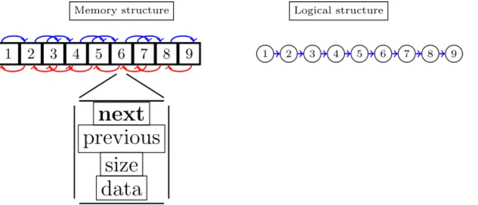
Nowadays multi-core computers get more and more processors, and the question is how to handle all this parallelism well. So, here’s a basic problem: Consider a doubly linked list that is shared by many processors. It supports insertions and deletions, and there are simple operations like summing up the size of the entries that should be done very fast. We decide to organize the data structure as an array of dynamic length, where each array index may or may not hold an entry. Each entry consists of the array indices of the next entry and the previous entry in the list, some basic information about the entry (e.g. its size), and a pointer to the lion’s share of the data, which can be anywhere in the memory.

1 2 3 4 5 6 7 8 9

Memory structure Logical structure

1 2 3 4 5 6 7 8 9

next previous

size data

Figure 1.1: Linked listed after initialization. Blue links are forward pointers, red links backward pointers (these are omitted from now on).

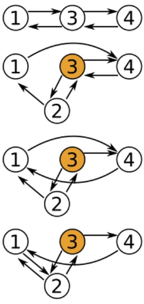
We now can quickly determine the total size by reading the array in one go from memory, which is quite fast. However, how can we do insertions and deletions fast? These arelocal operations affecting only one list entry and the pointers of its “neighbors,” i.e., the previous and next list element. We want to be able to do many such operations concurrently, by different processors, while maintaining the link structure! Being careless and letting each processor act independently invites disaster, see Figure 1.3.

1

(2)

. . . 1 2 3 4 5 6 7 8 9 . . .

1 4 2 5 3 6 8 7 9

Figure 1.2: State after many insertion and deletion operations. There may also be “dead” cells which are currently not part of the list. These are not shown;

we assume that these are taken care of every now and then to avoid wasting too much memory.

1 3 4

2 1 3 4

2

Figure 1.3: Concurrent insertion of a new entry 2 between 1 and 3, and (logical) deletion of entry 3. The deletion of 3 requires to change the successor and predecessor of 1 and 4, but the insertion of 2 changes the successor of 1 as well.

Not doing this in a consistent order messes up the list. Note that entry 3 might get physically deleted as well, rendering many of our pointers invalid.

On the other hand,anyset of concurrent modifications that doesnotinvolve neighbors is fine: The result is a neat doubly linked list. Clearly, we want to be able to manipulate arbitrary list entries. This can be rephrased as an (in)famous graph problem.

Problem 1.1(Vertex Coloring). Given an undirected graphG= (V, E), assign a color cu to each vertex u ∈ V such that the following holds: e = {v, w} ∈ E ⇒cv6=cw.

We then can “cycle” through the colors and perform concurrent operations on all “nodes” (a.k.a. list entries) of the same color without worrying. Once we’re done with all colors, we color the new list, and so on. We now have a challenging task:

• We want to use very few colors, so cycling through them is completed quickly. Coloring with a minimal number of colors is in general very hard,

(3)

1.1. THE PROBLEM 3

3

1 2

3

Figure 1.4: 3-colorable graph with a valid coloring.

but fortunately we’re dealing with a very simple graph.

• The coloring itself needs to be done fast, too. Otherwise we’ll be waiting for the new coloring to be ready all the time.

• That means we want to use all our processors. It’s easy to split up re- sponsibility for the list entries by splitting up the array. The downside of this is that the processors receive only fragmented parts of the list (see Figure 1.5).

• Trying to get consecutive pieces under the control of a single processor requires to break symmetry: List fragments get longer only if more nodes are added than removed. If the list is fragmented into single nodes, this roughly means that we want to find amaximal independent set, i.e., a set containing no neighbors to which we cannot add a node without destroy- ing this property. This turns out to be essentially the same problem as coloring, as we will see in the exercises.

. . . 1 2 3 4 5 6 7 8 9 . . .

Processor1 Processor2 Processor3

1 4 2 5 3 6 8 7 9

Figure 1.5: List split. We may get lucky in some places of the list (as for the blue processor), but in wide parts the list will be fragmented between processes.

As the list is fragmented among the processors anyway, it’s useful to pretend that we have as many processors as we want. That means each of the nodes can have its “own” processor! If we can deal with this case efficiently, it will cer- tainly work out with fewer processors! Oh, and one more thing: We have some additional information we can glean from the setup. Each node has a unique identifierassociated with it, namely its array index. Note that this means nodes already “look different” initially, which is crucial for coloring deterministically without starting from the endpoints only.

(4)

Remarks:

• In distributed computing, we often take the point of view that the system is a graph whose nodes are processors and whose edges are both representing relations with respect to the problem at hand and communication links.

This will come in handy here as an abstraction, but in many systems it is literally true.

• The assumption of unique identifiers is standard, the reason being that deterministic distributed algorithms can’t even do basic things without them (for instance coloring a list quickly). On the other hand, using randomization it’s trivial to generate unique identifiers with overwhelming probability. Nonetheless, it is also studied how important such identifiers actually are; more about that in another lecture!

• The linked list here is a toy example, but an entire branch of distributed computing is occupied with finding efficient data structures for shared memory systems like the one informally described above. We’ll have another look at such systems further into the course!

1.2 2-Coloring the List

Clearly, we can color the list with two colors, simply by passing through the list and alternating. Since this is sequential, i.e., only one process is actually working, it takes Θ(n) steps in a list ofnnodes. We can parallelize this strategy, however. For i∈[n] :={0, . . . , n−1}, denote byvi the array index of thei^th node in the list. As always in this course, log denotes the base-2 logarithm.

First, we add “shortcuts” to our linked list.

Algorithm 1Parallel pointer jumping

1: forj = 0, . . . ,dlogne −1 do

2: foreach nodevi in paralleldo

3: if i−2^j≥0 andi+ 2^j < nthen

4: {have nodevi create shortcuts betweenvi−2^j andvi+2^j}

5: store a pointer tovi−2^j at element vi+2^j 6: store a pointer tovi+2^j at element vi−2^j 7: end if

8: end for

9: end for

Here we assume that processes share a common clock to coordinate the execution of the outer loop, or somehow simulate this behavior. We’ll examine this issue more closely in the next lecture; let’s assume for now that we can handle this and call each iteration of the outer loop around.

Let’s have a closer look at what this algorithm does.

Lemma 1.2 (Shortcuts from pointer jumping). Afterrrounds of Algorithm 1, at each array index vi with i≥2^r the indexvi−2^r is stored. Likewise, at each index vi with i < n−2^r,vi+2^r is stored.

(5)

1.2. 2-COLORING THE LIST 5 Proof. We show the claim by induction. The base case isr= 0, i.e., the initial state. As 2⁰ = 1, the statement is just another way of saying that we have a doubly linked list, so we’re in the clear. Now assume that the claim is true for some 0≤ r < dlogne. In the r^th round, we have j = r−1. For any i ≥2^r, (the process responsible for) nodevi−2^r−1 will add vi−2^r to the entry at array index vi. It can do this, because by induction hypothesis vi−2^r and vi can be looked up at the array indexv_i−2^r−1. Note that processes dealing with aviwith i < 2^r−1 will not get confused: they will know that i <2^r−1 because v_i−2^r−1 was not added to the entry corresponding tovi. Similarly, for eachi < n−2^r, v_i+2^r−1 will add vi+2^r to the entry at indexvi.

1 4 2 5 3 6 8 7 9 1 4 2 5 3 6 8 7 9

Figure 1.6: Parallel pointer jumping. Depicted are the additional pointers/links of node 3 only.

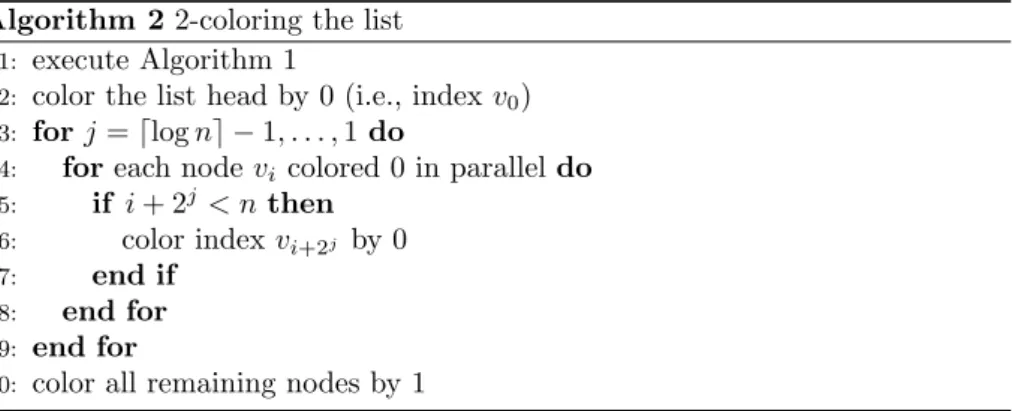
With these shortcuts, we can color the list quickly.

Algorithm 22-coloring the list

1: execute Algorithm 1

2: color the list head by 0 (i.e., indexv0)

3: forj=dlogne −1, . . . ,1 do

4: foreach nodevi colored 0 in paralleldo

5: if i+ 2^j< nthen

6: color indexvi+2^j by 0

7: end if

8: end for

9: end for

10: color all remaining nodes by 1

Theorem 1.3 (Correctness of Algorithm 2). Algorithm 2 colors the doubly linked list with2 colors.

Proof. From Lemma 1.2, we know that array elements will store the necessary information to execute the for-loops. By induction, we see that afterrrounds of the loop, all nodesviwithi mod 2^dlog^ne−r= 0 are colored 0. The loop runs fordlogne −1 rounds, i.e., until j = 1. Thus, all nodes in even distance from the list head are colored 0, while the remaining nodes get colored 1.

(6)

1 4 2 5 3 6 8 7 9 1 4 2 5 3 6 8 7 9

1 4 2 5 3 6 8 7 9

Figure 1.7: Execution of the 2-coloring algorithm. Each step uses a different

“level” of pointers constructed with the pointer jumping algorithm; the final steps just uses the neighbor pointers.

Remarks:

• In the above algorithms, we referred ton. However, nis unknown due to parallel insertions and deletions (maintaining a shared counter is another fundamental problem!). This can be resolved by lettingviterminatewhen it knows that its work is done, which is the case when not bothvi−2^j and vi+2^j are written toviin roundj. The processors then just need to notify each other once all their associated nodes are terminated.

• For 2-coloring, the O(logn) rounds of this algorithm are the best we can get: another straightforward induction shows that following pointers, it takes dlogherounds to “see” something that ish“hops” in the list away, and unless individual processors read large chunks of memory, this has to be done.

• The issue is that 2-coloring is too rigid. Once we color a single node, all other nodes’ colors are determined. The problem is notlocal.

• This is also bad for another reason: if we have only small changes in the list, we would like to avoid having to recolor it from scratch. It would be nice to have an algorithm where the output depends only on a small number of hops around each node. This would most likely also yield a fast and efficient algorithm!

• We can use the pointer jumping technique to speed up algorithms that are more local in this sense: if in round r nodes write everything they know to the array entries of nodes in distance 2^r⁻¹, it takes only dloghe steps until the output of an algorithm depending on nodes in distance at mosthcan be determined. However, this is only practical ifhis small, as otherwise a lot of work is done!

1.3 Using 3 Colors

What good does it do to get down to two colors, but at a large overhead?

None, as we have to do it again after each change of the list. Let’s be a bit more relaxed and permit c > 2 colors. This means that, no matter what the neighbors’ colors are, there’s always a free one to pick! Given that we start with a valid coloring – the array indices – we can use this to reduce the number of colors to 3. Let’s assume in the following that v₋1 =vn−1 and vn =v0 (i.e.,

(7)

1.3. USING 3 COLORS 7 head and tail of the list also have pointers to each other), since this will simplify describing algorithms.

Algorithm 3color reduction

2: cvi:=vi 3: end for

4: while ∃vi:cvi >2 do

5: foreach nodevi withcv_i>max{cvi−1, cv_i+1,2}in paralleldo

6: cv_i:= min [3]\ {cvi−1, cv_i+1}

7: end for

8: end while

Lemma 1.4. Algorithm 3 computes a 3-coloring. It terminates in c rounds, wherec is the number of different colors in the initial coloring (here n, because the array indices are unique).

Proof. No two neighbors can change their color in the same round, as this would require that each of their colors is larger than the other. Thus, the coloring is valid after each round (given that it was valid initially). A node with the current maximum color will change its color (because no neighbor can have this color, too). Note also that no colors other than 0, 1, or 2 are ever picked by a node.

It follows that the algorithm completes after at mostcrounds and the result is a valid 3-coloring.

Remarks:

• A time complexity of (almost)nrounds is attained if we still have a nice, well-ordered list, i.e.,vi =ifor alli. In other words, if we’re unlucky, we color the list sequentially.

• The algorithm is, however, good to reduce the number of colors to 3 if we only have a few colors to begin with.

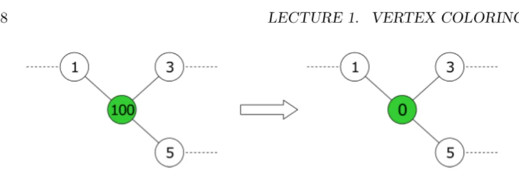
• If we have an arbitrary graph of maximum degree ∆ (i.e., no node has more than ∆ neighbors), the same approach can be used to find a (∆ + 1)- coloring (see Figure 1.8).

• It’s not hard to show that if the initial coloring is random, the algorithm will finish in Θ(logn/log logn) rounds with a very large probability. Can you prove it?

• One can construct such an initial coloring by picking colors randomly at each node from a sufficiently large range.

• Combining with pointer jumping, we get a running time of Θ(log logn) for 3-coloring, exponentially faster than for 2-coloring!

(8)

Figure 1.8: Vertex 100 receives the lowest possible color.

1.4 Cole-Vishkin

The previous algorithm reduced the number of colors in each step, starting from a valid coloring. We can now ask: Can this be done more quickly/efficiently?

The answer turns out to be yes, as shown by the following algorithm, which is based on a simple, but ingenious idea.

Algorithm 4Cole-Vishkin color reduction

2: cvi:=vi 3: end for

4: while ∃vi:cvi >5 for all nodes in paralleldo

5: interpret cvi andcvi−1 as (infinite) little-endian bit-strings, i.e., starting with the least significant bit

6: letj be the smallest index where they differ

7: concatenate the differing bit itself and j (encoded as bitstring), yielding colorc

8: cv_i:=c

9: end while Example:

Part of an execution of Algorithm 4, written in little-endian (least significant bit is far left):

v_i−2 0000110100 → . . . → . . . v_i−1 0000100101 → 01010 → . . . vi 0000100110 → 10001 → 1000

The trick is that either the first or the second part of (the bit string of) the new color saves the day.

Lemma 1.5 (Correctness of Cole-Vishkin). Algorithm 4 computes a valid coloring.

Proof. Since the initial coloring is valid, we need to show that a valid coloring enables to compute the new colors and the new coloring is valid. The first part readily follows from the fact that two different colors must have differing bit strings, so the index j can be computed. Now consider two neighbors vi and vi−1. If they determine different indices j for which the current colors differ from vi−1 and vi−2 respectively, the front part of the new colors is different.

(9)

1.4. COLE-VISHKIN 9 Otherwise, the “least significant differing bit” part of their new colors implies a differing bit!

This algorithm terminates in (almost) log^∗n time. Log-Star is thenumber of times one needs to take the logarithm (to the base 2) to get to at most 1, starting withn:

Definition 1.6 (Log-Star).

∀x≤1 : log^∗x:= 0 ∀x >1 : log^∗x:= 1 + log^∗(logx)

Theorem 1.7. Algorithm 4 computes a valid6-coloring inlog^∗n+O(1)rounds.

Proof. Correctness is shown in Lemma 1.5. The time complexity follows from the fact that if the original color hadbbits, the new color has at mostdlogbe+ 1 bits: the number of bits to encode an index in ab-bit string plus the appended bit. The O(1) term addresses the fact that we don’t actually apply the base- 2 logarithm in each step. (The non-exciting computations showing that this makes only a minor difference are omitted.) The reason why we end up with 6 colors is simple: encoding an index of a 3-bit value yields 00, 01, or 10 as leading parts; appending a bit yields 6 possibilities. It’s simple to check that for any larger number of initial colors, fewer possibilities will remain.

Remarks:

• Log-star is an amazingly slowly growing function. Log-star of all the atoms in the observable universe (estimated to be 10⁸⁰) is 5. Hence, for all practical purposes, it’s constant.

• One can use Algorithm 3 to reduce the number of colors to 3 in 3 rounds.

• As stated, the algorithm has a termination condition that cannot be checked efficiently based on local information. Fortunately, we can just get rid of this condition and run the algorithm for the right number of rounds given by Theorem 1.7.

• This does not work ifnis unknown. This issue has two different solutions:

a practical one and a theoretical one. Can you figure out both?

• For a change, the O(1) term is actually hiding only a small constant.

The time complexity of the problem has been nailed down to be precisely 1/2·log^∗nfor infinitely many values ofn[RS15].

• Another detail here is that instead of n, the argument of the log^∗ is, in fact, the initial range of colors. In our case, this is the current size of the array, which may be larger thann, typically by some constant factor.

However, even if it would be exponentially larger, this would mean we need to do just one or two more rounds of the algorithm to handle this.

• A simple modification results in running time 1/2 ·log^∗n+O(1) (see exercises).

• Using pointer jumping, the running time can be reduced to log(log^∗n) + O(1). Shockingly, this isnot the most ridiculously slow-growing function I’ve encountered in a statement that is not deliberately about slow-growing functions.

(10)

• The technique is not limited to lists. It can be used to color oriented trees and constant-degree graphs inO(log^∗n) rounds, too (see exercises).

1.5 Linial’s Lower Bound

If we can color the listthat fast, can’t we find an algorithm that does it in truly constant time? The answer is no, and we’re going to see now why. We’ll focus on the case where interactions are solely with neighbors, in which one requires Ω(log^∗n) rounds. Such algorithms are called message-passing algorithms, for reasons that will be discussed in the next lecture. With shared memory, the variant of Cole-Vishkin with pointer jumping is asymptotically optimal [FR90].

We also restrict to deterministic algorithms.

Before we do the proof, let’s simplify the situation a bit. First, observe that all information the output of vi can be influenced by in a T-round message passing algorithm is the information that’s initially available at nodes v_i−T, v_i−T+1, . . . , vi+T. In the worst case, every content stored is identical,¹ so the only real difference are the actual array indices (and memory addresses).

Note also that the order is relevant: We have forward and backward pointers, i.e., we can distinguish directions, and obviously it’s possible to count the number of “hops” traversed. Consequently, even if we don’t know anything about a coloring algorithm except that it is a deterministic T-round algorithm A(with neighbor-neighbor interactions only), we can conclude that there is a function

f: (x0, . . . , x2T)→[c]

so thatcv_i =f(vi−T, vi−T+1, . . . , vi+T) when executingA. Here,cis the number of colors used byAand we assume without loss of generality (w.l.o.g.) that [c]

is the set of colors produced by the algorithm.²

x₁ x₂ x₃ x₄ x₅ f(x₁, x₂, x₃, x₄, x₅)

Figure 1.9: Interpreting a 2-round coloring algorithm as a coloring function f mapping 5-tuples to colors.

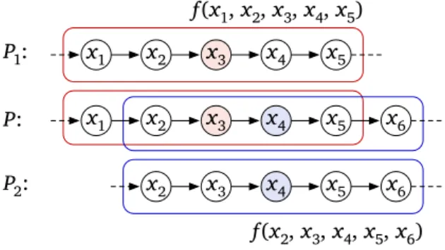
IfAproduces a valid coloring, we also know that f(x0, . . . , x2T)6=f(x1, . . . , x2T+1)

provided thatxi6=xjfori6=j,i, j∈[2T+ 2]: The two arguments could be the views of adjacent nodes in the list, and they must not compute the same color.

Now comes the clever bit making our lives much easier: We restrict the problem without actually taking away what makes it hard. This will simplify our key argument, as it has an algorithmic component – and it would be more

1Even if that wasn’t true, the same argument applies taking this content into account.

2As opposed to, e.g.,{pink, elephant, turtle}.

(11)

1.5. LINIAL’S LOWER BOUND 11 challenging to come up with an algorithm for the more general setting. For c, k∈N, we say that gis a k-aryc-coloring function if

∀0≤x1< x2< . . . < xk < n: g(x1, x2, . . . , xk)∈[c]

and

∀0≤x1< x2< . . . < xk+1< n: g(x1, x2, . . . , xk)6=g(x2, x3, . . . , xk+1).

Fork= 2T+ 1, these are the exact same requirements as tof, however, only for ascending addressesx1< . . . < xk+1< n. Note that by restricting the domain off to such inputs, we see that the existence of aT-round algorithmAusingc colors implies the existence of a (2T+ 1)-ary c-coloring functionf.

x₁ x₂ x₃ x₄ x₅ x₆ x₁ x₂ x₃ x₄ x₅

x₅ x₃ x₄

x₂ x₆

P:

P₁:

P₂:

f(x₁, x₂, x₃, x₄, x₅)

f(x₂, x₃, x₄, x₅, x₆)

Figure 1.10: 5-tuples that correspond to possible views of adjacent nodes must result in different colors.

Using this connection, we can now move on to the proof of the lower bound, which consists of showing that ifcis small, thenT cannot be arbitrarily small, too.

Lemma 1.8 (1-ary functions require many colors). If f is a 1-ary c-coloring function, thenc≥n.

Proof. By definition,f(x1)6=f(x2) for all 0≤x1< x2< n, i.e.,

∀x16=x2∈[n] : x16=x2⇔f(x1)6=f(x2).

In other words,f is an injection, which is only possible ifc≥n.

The main step of the proof is to show that we can construct (k−1)-ary 2^c-coloring functions out of k-ary c-coloring functions. That is, we can “pay”

for saving time by using more colors.

Lemma 1.9 (k-aryc-coloring enables (k−1)-ary 2^c-coloring). If f is a k-ary c-coloring function for some k > 0, then a (k−1)-ary2^c-coloring function g exists.

Proof. First, lethbe a bijection from the subsets of [c] to [2^c]. Concretely, we may choose for S ⊆[c] as h(S) the string of c bits in which the i^th bit is 1 if and only ifi−1∈S (but any other bijection would do, too).

(12)

Next, define

g⁰(x1, . . . , xk−1) :={f(x1, . . . , xk)|xk−1< xk < n},

i.e.,g⁰ is thesetof all colors that can possibly be assigned byf when all but the last argument off are specified. These are the colors that might cause trouble whengassigns a color tox1, . . . , xk−1without consideringxk. Usingh, we can interpret this set as a new color:³

g(x1, . . . , xk−1) :=h◦g⁰(x1, . . . , xk−1) =h(g⁰(x1, . . . , xk−1)).

It’s straightforward to check that this is a well-defined function with range [2^c]:

g⁰(x1, . . . , xk−1) ⊆ [c] and h maps such sets to a color from [2^c]. In order to verify that g is indeed a (k−1)-ary 2^c-coloring function, we thus must show that

∀0≤x1< x2< . . . , xk < n: g(x1, . . . , xk−1)6=g(x2, . . . , xk).

Let 0 ≤ x1 < x2 < . . . < xk < n. Clearly, f(x1, . . . , xk) ∈ g⁰(x1, . . . , x_k−1).

On the other hand, we have that f(x1, . . . , xk) 6= f(x2, . . . , xk+1) for any xk < xk+1 < n, because f is a coloring function. This is equivalent to saying that f(x1, . . . , xk) ∈/ g⁰(x2, . . . , xk). We conclude that g⁰(x1, . . . , xk−1) 6= g⁰(x2, . . . , xk). Sincehis a bijection, this is equivalent to

g(x1, . . . , x_k−1) =h(g⁰(x1, . . . , x_k−1))6=h(g⁰(x2, . . . , xk)) =g(x2, . . . , xk).

With these lemmas, it’s a piece of cake to obtain the lower bound.

Theorem 1.10(Linial’s lower bound). Coloring a list with a message passing algorithm that uses (at most) 4 colors requires at least1/2·log^∗n−1rounds.

Proof. Assume thatAis aT-round coloring algorithm using 4 colors. Thus, a (2T+1)-ary 4-coloring function exists. We apply Lemma 1.9 for 2Ttimes, to see that then a 1-ary (^2T2)⁴-coloring function exists. Here,^a2 denotes the tetration or “power tower,” the a-fold iterated exponentiation by 2. From Lemma 1.8, we know that

2T+22 = ^2T2⁴

≥n, yielding

2T+ 2≥log^∗n and finally

T ≥log^∗n 2 −1.

3Note thathdoesn’t really do anything but “rename” the sets such that they are easy to count. That’s why, rather than turtles or sets, we like our colors to be numbers!

(13)

1.5. LINIAL’S LOWER BOUND 13 Remarks:

• More colors don’t help a lot. If we consider c colors in the above proof, we get that it requires at least 1/2·(log^∗n−log^∗c) rounds to color with c colors.

• Randomization doesn’t help either. Naor extended the lower bound to randomized algorithms [Nao91].

• I’ve been a bit sloppy, as I haven’t defined the model precisely. This can easily lead to mistakes, so I will make amends in the next lecture. The given proof works in the so-called message passing model, which we get to know in more detail in the next lecture.

• If one permits non-neighbor interactions, the lower bound weakens to dlog(1/2·(log^∗n−log^∗c))e[FR90], just like we could speed up the Cole- Vishkin algorithm using pointer jumping.

What to take Home

• Exploiting parallelism, distributed algorithms can be extremely fast.

• Symmetry breaking is a fundamental challenge in distributed computing, and a coloring is a basic structure that breaks symmetry between neighbors.

• The key to understanding parallelism is to understand what is possible based on limited (in particular local) information.

• What can and can’t be done is quite sensitive to the model. When consid- ering running time bounds, impossibility results, etc. it is thus important to keep in mind that changing an aspect of the model may have a dramatic impact. Try always to understand what aspects of a model cause a certain result, and wonder whether changing them would change the game!

• On the other hand, we can frequently prove unconditional lower bounds in distributed computing, such as Theorem 1.7. If wedo figure out what the suitable model of computation is for a given system, we may be able to understand precisely how fast things can be done. Contrast this with lower bounds on sorting (which restrict the feasible operations) or impossibilities in the sequential world that rest on conjectures like P6= NP or the unique games conjecture!

• Math is going to be our friend in this lecture. If your reflex is to disagree, try to imagine figuring out how fast the list can be colored by concurrent processes without the tools we used. Moreover, coming up with a proof requires us to reflect on our assumptions and crystallize ideas; that’s dif- ficult, but very useful when dealing with more complex problems later on!

(14)

Bibliographic Notes

The basic technique of the log-star algorithm is by Cole and Vishkin [CV86].

The technique can be generalized and extended, e.g., to a ring topology or to graphs with constant degree [GP87, GPS88, KMW05]. Using it as a subroutine, one can solve many problems in log-star time.

The lower bound of Theorem 1.7 is due to Linial [Lin92]. Linial’s paper also contains a number of other results on coloring, e.g., that any message passing algorithm for coloring d-regular trees of radius r that runs in time at most 2r/3 requires at least Ω(√

d) colors. The presentation here is based on a more streamlined version by Laurinharju and Suomela [LS14].

Figures 1.9 and 1.10 are courtesy of Jukka Suomela and under a creative commons license.⁴ Figures 1.4 and 1.8 are courtesy of Roger Wattenhofer;

substantial parts of today’s lecture are based on material from his course at ETH Zurich. Wide parts of today’s lecture are covered by books [CLR90, Pel00].

Bibliography

[CLR90] Thomas H. Cormen, Charles E. Leiserson, and Ronald L. Rivest.

Introduction to Algorithms. The MIT Press, Cambridge, MA, 1990.

[CV86] R. Cole and U. Vishkin. Deterministic coin tossing and accelerating cascades: micro and macro techniques for designing parallel algorithms. In 18th annual ACM Symposium on Theory of Computing (STOC), 1986.

[FR90] Faith E. Fich and Vijaya Ramachandran. Lower bounds for parallel computation on linked structures. InProc. 2nd Annual ACM Sympo- sium on Parallel Algorithms and Architectures (SPAA 1990), pages 109–116, 1990.

[GP87] Andrew V. Goldberg and Serge A. Plotkin. Parallel (∆+1)-coloring of constant-degree graphs. Inf. Process. Lett., 25(4):241–245, June 1987.

[GPS88] Andrew V. Goldberg, Serge A. Plotkin, and Gregory E. Shannon.

Parallel Symmetry-Breaking in Sparse Graphs. SIAM J. Discrete Math., 1(4):434–446, 1988.

[KMW05] Fabian Kuhn, Thomas Moscibroda, and Roger Wattenhofer. On the Locality of Bounded Growth. In 24th ACM Symposium on the Principles of Distributed Computing (PODC), Las Vegas, Nevada, USA, July 2005.

[Lin92] N. Linial. Locality in Distributed Graph Algorithms. SIAM Journal on Computing, 21(1)(1):193–201, February 1992.

[LS14] Juhana Laurinharju and Jukka Suomela. Brief Announcement:

Linial’s Lower Bound Made Easy. In Symposium on Principles of Distributed Computing (PODC), pages 377–378, 2014.

4CC BY-SA 3.0, seehttps://creativecommons.org/licenses/by-sa/3.0/.

(15)

BIBLIOGRAPHY 15 [Nao91] Moni Naor. A Lower Bound on Probabilistic Algorithms for Distribu-

tive Ring Coloring. SIAM J. Discrete Math., 4(3):409–412, 1991.

[Pel00] David Peleg. Distributed computing: a locality-sensitive approach.

Society for Industrial and Applied Mathematics, Philadelphia, PA, USA, 2000.

[RS15] Joel Rybicki and Jukka Suomela. Exact bounds for distributed graph colouring. CoRR, abs/1502.04963, 2015.

(16)