SURFACE AIR TEMPERATURE AND ITS CHANGES OVER THE PAST 150 YEARS

THE PAST 150 YEARS

P. D. Jones,

M. New,

D. E. Parker,

S. Martin,

and I. G. Rigor

Abstract. We review the surface air temperature record of the past 150 years, considering the homogene- ity of the basic data and the standard errors of estima- tion of the average hemispheric and global estimates.

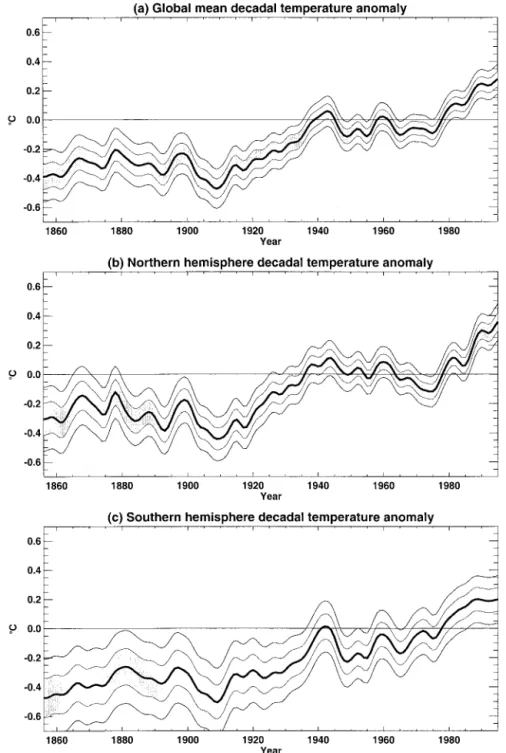
We present global fields of surface temperature change over the two 20-year periods of greatest warming this century, 1925–1944 and 1978–1997. Over these periods, global temperatures rose by 0.37 8 and 0.32 8 C, respec- tively. The twentieth-century warming has been accom- panied by a decrease in those areas of the world affected by exceptionally cool temperatures and to a lesser extent by increases in areas affected by exceptionally warm temperatures. In recent decades there have been much greater increases in night minimum temperatures than in day maximum temperatures, so that over 1950–1993 the diurnal temperature range has decreased by 0.08 8 C per decade. We discuss the recent divergence of surface

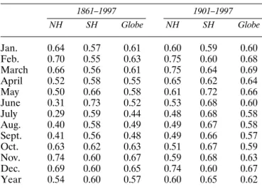
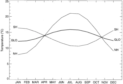
and satellite temperature measurements of the lower troposphere and consider the last 150 years in the con- text of the last millennium. We then provide a globally complete absolute surface air temperature climatology on a 1 8 3 1 8 grid. This is primarily based on data for 1961–1990. Extensive interpolation had to be under- taken over both polar regions and in a few other regions where basic data are scarce, but we believe the climatol- ogy is the most consistent and reliable of absolute sur- face air temperature conditions over the world. The climatology indicates that the annual average surface temperature of the world is 14.0 8 C (14.6 8 C in the North- ern Hemisphere (NH) and 13.4 8 C for the Southern Hemisphere). The annual cycle of global mean temper- atures follows that of the land-dominated NH, with a maximum in July of 15.9 8 C and a minimum in January of 12.2 8 C.

1. INTRODUCTION

The surface air temperature database has been exten- sively reviewed on several earlier occasions, most nota- bly by Wigley et al. [1985, 1986] and Ellsaesser et al. [1986]

and by the Intergovernmental Panel on Climate Change (IPCC) [Folland et al., 1990, 1992; Nicholls et al., 1996].

This work extends these by using slight improvements to the basic surface database and updates the records to the end of 1998. Most importantly, it also provides a com- prehensive analysis of surface air temperatures in abso- lute rather than anomaly units, by the development of a 1 8 by 1 8 grid box climatology for all land, ocean, and sea ice areas based on the 1961–1990 period.

The structure of this review is as follows. Section 2 discusses the quality of the raw land and marine tem- perature data, addressing the long-term homogeneity of the basic data and considering those subtle changes that might influence the data, such as urbanization of land

areas and gradual changes in observing practices over the ocean. Section 3 reviews several methods that have been used to aggregate the basic data to a regular grid, the basic aim of which is to reduce the effects of spatial and temporal variations in the spatial density of avail- able data. Future improvements to the network are discussed.

Before consideration of what the data tell us about the post-1850 instrumental era, section 4 assesses the accuracy of the estimates of hemispheric and global temperature anomalies, particularly during the nine- teenth century, when coverage was poorer. Section 5 then analyzes the surface temperature record. It com- pares patterns of warming over the 1978–1997 period with those of the earlier 1925–1944 period, which expe- rienced a comparable rate of warming. It also considers trends in the areas affected by extreme temperatures, recent trends in Arctic temperatures and in maximum and minimum temperatures, the recent divergence of surface temperature trends and satellite retrievals of lower tropospheric temperature trends, and the last 150 years in a longer near-millennial context.

The discussion in section 5 is limited to what the surface record tells us about past temperature changes.

Extensive discussion of the reasons for the changes (both variations in atmospheric circulation and past external

1

Climatic Research Unit, University of East Anglia, Nor- wich, England.

2

Hadley Centre, Meteorological Office, Bracknell, England.

3

School of Oceanography, University of Washington, Seattle.

4

Applied Physics Laboratory, University of Washington, Seattle.

Copyright 1999 by the American Geophysical Union. Reviews of Geophysics, 37, 2 / May 1999 pages 173–199

8755-1209/99/1999RG900002$15.00 Paper number 1999RG900002

●

173

forcing) may be found in the IPCC assessments [Folland et al., 1990, 1992; Nicholls et al., 1996] and elsewhere [e.g., van Loon and Williams, 1976; Karl et al., 1989, 1993a; Trenberth, 1990; Parker et al., 1994; and Hurrell, 1995]. In section 6 the development of the absolute climatology is described, and section 7 presents our conclusions.

2. HOMOGENEITY OF THE BASIC DATA

However mathematically cunning or appealing an analysis technique may be, any results or conclusions are dependent upon the quality of the basic data. In clima- tology, quality of the data is essential. A time series of monthly temperature averages is termed homogeneous [Conrad and Pollak, 1962] if the variations exhibited by the series are solely the result of the vagaries of the weather and climate. Many factors can influence homo- geneity, which we next discuss by division of the surface data into land and marine components.

2.1. Land Component

The most important causes of inhomogeneity are (1) changes in instrumentation, exposure, and measurement technique; (2) changes in station location (both position and elevation); (3) changes in observation times and the methods used to calculate monthly averages; and (4) changes in the environment of the station, particularly with reference to urbanization that affects the represen- tativeness of the temperature records. All of these have been discussed at length in the literature [see, e.g., Mitchell, 1953; Bradley and Jones, 1985; Parker, 1994]. A number of subjective and relatively objective criteria [e.g., Jones et al., 1985, 1986a, b, c; Easterling and Peter- son, 1995; Alexandersson and Moberg, 1997] exist for testing monthly data. Peterson et al. [1998a] provide a comprehensive review of these and numerous other techniques.

Here we use the land station data set developed by Jones [1994]. All 2000 1 station time series used have been assessed for homogeneity by subjective interstation comparisons performed on a local basis. Many stations were adjusted and some omitted because of anomalous warming trends and/or numerous nonclimatic jumps (complete details are given by Jones et al. [1985, 1986c]).

All homogeneity assessment techniques would per- form poorly if all station time series were affected sim- ilarly by common factors (e.g. those related to urbaniza- tion). Urban development around a meteorological station means that measured temperatures are slightly warmer than they would otherwise have been. The effect is a real (rather than spurious as in the other causes of inhomogeneities) change in climate. It is considered an inhomogeneity, however, as the measured temperatures are no longer representative of a larger area. The ur- banization influence we are interested in is the effect on the monthly time series. This effect is considerably

smaller than individual daily or even hourly occurrences.

Effects up to 10 8 C, for individual days, have been quoted for some cities [see, e.g., Oke, 1974]. To assess urban- ization influences on monthly and longer timescales in certain regions (Australia [Torok, 1996]; Sweden [Moberg and Alexandersson, 1997]), specific rural station data sets have been developed to allow estimation of the magnitude of possible residual urban warming influ- ences in the Jones [1994] data set. Results show that if there are residual influences, they are an order of mag- nitude smaller than the nearly 0.6 8 C warming evident during the twentieth century, confirming earlier work [Jones et al., 1989, 1990; Karl and Jones, 1989].

2.2. Marine Component

Historical temperature data over marine regions are largely derived from in situ measurements of sea surface temperature (SST) and marine air temperature (MAT) taken by ships and buoys. Inhomogeneity problems with both variables relate principally to changes in instrumen- tation, exposure, and measurement technique. For SST data the change in the sampling method from uninsu- lated buckets to engine intakes causes a rise in SST values of 0.3 8 –0.7 8 C [James and Fox, 1972]. Engine in- take measurements dominate after the early 1940s with uninsulated bucket measurements the main method be- fore. For MAT data, the average height of ships’ decks above the ocean surface has increased during the present century, but the more serious problem is the contamination of daytime MAT through solar heating of the ships’ infrastructure, rendering only the nighttime MAT (NMAT) data of value [Parker et al., 1994, 1995a].

Folland and Parker [1995] developed a model to esti- mate the amount of cooling of the seawater that occurs in buckets of various types, depending upon the time between sampling and measurement and the ambient weather conditions. Adjustments to the bucket SST val- ues for all years before 1941 are estimated on the basis of assumptions about the sampling time and the types of bucket in use at different times. The adjustments, which are greater in winter, are tuned using an assumption that SST annual cycle amplitudes have not experienced a longer-term trend [Folland and Parker, 1995]. Canvas buckets, which evaporatively cool more than wooden buckets, were in dominant use after the late nineteenth century, having gradually replaced the wooden buckets that would have been used initially in the mid nineteenth century. Some buckets are still in use today, but since the early 1940s they have been much better insulated, al- though it is believed that uninsulated buckets were still used on some ships until the 1960s (C. K. Folland, personal communication, 1995.).

In the combination of marine data with land-based

surface temperatures, SST anomalies are used in pref-

erence to NMAT because they are considered more

reliable [Trenberth et al., 1992]. The basic assumption is

that on monthly and longer timescales an anomaly value

of SST will be approximately equal to that of the air

immediately (typically 10 m) above the ocean surface (NMAT). The rationale is that SST observations are more reliable [Parker et al., 1995a] throughout the world.

Fewer individual SST than MAT readings per unit area would be required to give averages of the same reliabil- ity, owing to the stronger day-to-day autocorrelation in SST compared with MAT values [see Parker, 1984], even if the MAT observations had been as reliable as those of SST. In practice, the number of usable MAT observa- tions is only about half that of SST.

The independence of the land and marine compo- nents of the surface temperature record means that hemispheric and regional series can be used to test the veracity of the other component. The components have been shown to agree with each other on the hemispheric basis by Parker et al. [1994] and, using island and coastal regions in the southwestern Pacific, by Folland and Salin- ger [1995] and Folland et al. [1997].

3. AGGREGATION OF THE RAW DATA 3.1. Land Component

Several different methods have been used to interpo- late the station data to a regular grid. Peterson et al.

[1998b] recognize three current and different tech- niques: (1) the reference station method (RSM) used by Hansen and Lebedeff [1987], (2) the climate anomaly method (CAM) used by Jones [1994], and (3) the first difference method (FDM) used by Peterson et al.

[1998b].

The CAM technique differs from the other two in requiring that each station be reduced to anomalies from monthly means calculated for a common period. Jones [1994] uses 1961–1990, requiring each station to have at least 20 years of values from the base period, and esti- mates mean values, where possible using nearby series, for stations that have long records but that do not have 20 years data during 1961–1990. Station temperature anomaly values are then averaged together for all sta- tions within each 5 8 3 5 8 grid box. Resulting grid box time series differ in the number of stations between grid boxes and through time. Individual grid box time series may therefore have differences in variances with time due to changes in station numbers. The implications of this are discussed in sections 4 and 5.

In the RSM technique, the world is divided into a number of areas (Hansen and Lebedeff [1987] use 80), and a key long station is selected, where possible, in each area. Within each area, successively shorter station records are adjusted so that their averages equal the composite of all stations already incorporated over the overlap with the composite. The method enables all records to be used provided that they have a reasonable length of overlap (e.g., 10 years) with the composite.

Differences in variance of the area average series will also be present owing to changes in time of station numbers.

The FDM is the newest approach and works on the first difference (FD) time series, the difference in tem- perature between successive values in a station time series, e.g., Jan(t) minus Jan(t 2 1). FD values are averaged together for all stations within each 5 8 3 5 8 grid box as with the CAM technique. To revert to a similar analysis as CAM, the cumulative sum of each grid box series is calculated. The resulting series there- fore have similar potential changes in variance due to changing station numbers between and within boxes as in CAM. This aspect will also be present in RSM series, but to a lesser extent.

In all three techniques, large-scale hemispheric and global series are computed by a weighted average of all the grid boxes with data. For CAM and FDM the weights are the cosine of the central latitude of the grid box, while for RSM the box size was chosen to be of approximately equal area. Peterson et al. [1998b] show that the differences between the methods for trends over the 1880–1990 period are only a few hundredths of a degree Celsius per 100 years, the differences being due more to differences in techniques for calculation of a linear trend than to differences between the three meth- ods. The three methods also differ somewhat in their interannual variances. CAM and FDM have similar vari- ances, but the RSM has a significantly smaller variance [Peterson et al., 1998b].

A fourth approach, optimal interpolation, has been proposed by Vinnikov et al. [1990]. The approach is based on pioneering Russian work on the averaging of meteorological fields (recently published in English by Kagan [1997]). Regional and hemispheric averages and their errors are computed directly and it is not necessary to calculate grid box values. The most recent example of its use is by Smith et al. [1994] in the calculation of average global sea surface temperature.

3.2. Marine Component

For marine regions the raw data must be aggregated in a different manner. Each SST or NMAT value is accompanied by location data. Climatological monthly fields for each 1 8 square and for each pentad (5-day period) and day of the year were calculated on the basis of all in situ data from the 1961–1990 period. For SST a background climatology based partly on satellite data, adjusted to be unbiased relative to the in situ data, was used to guide interpolation of data voids in each indi- vidual month in 1961–1990 [Parker et al., 1995a, b].

These complete monthly fields were then smoothed

slightly in an attempt to reduce errors in regions when

there are few observations before averaging over the 30

years. Harmonic interpolation was then used to generate

the pentad climatology, which was then linearly interpo-

lated to the daily timescale. Grid box (5 8 3 5 8 ) anomalies

for each month are now produced by trimmed averaging

of all 1 8 anomalies (from their respective daily average)

for each of the pentads that make up the month. The

trimming removes the effects of outliers. A final check is

then made for unreasonable outliers, on a monthly basis, by assessing whether 5 8 grid box anomalies deviated by more than 2.25 8 C from the average of the eight neigh- bors in space (of which four had to be nonmissing to make the test) or time (of which both the previous and next months had to exist to perform the test). If the value failed the test, it was replaced by the neighbor average. The 2.25 threshold was chosen empirically:

higher thresholds admitted bull’s eyes; lower thresholds caused deletion of possibly correct values. Full details of the method are given by Parker et al. [1995a, b]. The grid box anomalies are based only on in situ measurements from ships and buoys; no satellite data are used.

3.3. Combination of Land and Marine Components The two data sets used are Jones [1994] for the land areas and Parker et al. [1995a] for the oceans. Both have been produced on the same 5 8 3 5 8 grid box basis. In the combined data set, the two data sets are merged in the simplest fashion. Anomaly values are taken, where avail- able, from each component. For grid boxes where both components are available, the combined value is a weighted one, with the weights determined by the frac- tions of land and ocean in the box. Because the land component for oceanic islands is potentially more reli- able than surrounding SST values, the land fraction is assumed to be at least 25% for each of the island and coastal boxes. A corresponding condition is applied to the ocean fraction in boxes where this is less than 25%.

The method is described in more detail by Parker et al.

[1994, 1995a].

3.4. Hemispheric and Global Anomaly Time Series Figure 1 shows the two hemispheric time series by season and year. The global annual series exhibits a warming (estimated by a linear trend calculation using least squares) of 0.57 8 C over the 1861–1997 period. On these large spatial scales, the series shown agree with more recent analyses [e.g., Peterson et al., 1998b], attest- ing to some extent that the homogeneity exercise of the previous section has been successful. Different station temperature compilations never use exactly the same basic land station and marine data, but the vast majority ( . 98%) of the basic data is in common.

Table 1 gives monthly trend values for each hemi- sphere and the globe computed over the 1861–1997 and 1901–1997 periods. Trends for all months, seasons, and years in both periods are significant at better than the 99% level. Estimation of the changes over the last 137 years using linear trends is just one method that can be used. All monthly, seasonal and annual series are poorly approximated by linear trends, particularly in the North- ern Hemisphere (NH). Alternatives, using the differ- ences between the first and last 10- or 20-year periods, however, give similar results. The estimated trends are also partly dependent upon the starting and ending years and the period used (see also Karl et al. [1994]). Trends

would be slightly larger using, for example, the period since 1881.

Warming evident in Table 1 is slightly greater for both periods for the Southern Hemisphere (SH), but there are greater seasonal differences in the NH com- pared with the SH. The global series is calculated as the average of the two hemispheric series. Nicholls et al.

[1996] calculate the global series as the weighted sum of all grid boxes. The latter method can bias the global average to the NH value when there are marked differ- ences in hemispheric coverage, but the effect is relatively small [Wigley et al., 1997].

In the Northern Hemisphere, Figure 1 shows that year-to-year variability is clearly greater in winter than in summer. The greater variability in all seasons in both hemispheres during the years before 1881 is due princi- pally to the sparser data available during these years and represents greater uncertainty in the estimates (see also section 4). This feature is much more marked in the Northern Hemisphere, especially over the land regions [e.g., Jones, 1994]. Both hemispheres clearly exhibit two periods of warming: 1920–1940, especially in the North- ern Hemisphere, and since the mid-1970s in both hemi- spheres. In the global annual series (Figure 2), 10 of the 12 warmest years occur between 1987 and 1998. The two years not occurring in this period are 1944 and 1983. The warmest year of the entire series on a global basis occurred in 1998, 0.57 8 C above the 1961–1990 average.

The next warmest years were 1997 (0.43 8 C), 1995 (0.39 8 C), and 1990 (0.35 8 C). More discussion of the database will be undertaken in section 5.

3.5. Future Improvements to the Database

At present only ; 1000 station records are used to monitor air temperatures over land regions [Jones, 1994]. This represents an apparent reduction by nearly a factor of 2 from the number available during the 1951–

1980 period, but this reduction is principally in areas of good or reasonable station coverage. The reduction stems from the greater availability of past data in some countries (e.g., United States, Canada, former Soviet Union (fUSSR), China and Australia), data that are not available in real time.

The reduction in land data availability does not seri-

ously impair hemispheric temperature estimates, but it

does reduce the quality of the grid box data set and the

quality of subregional series, particularly in the tropics

[Jones, 1995a]. Efforts are currently under way to im-

prove the land component of the data set. Nearly 1000

sites have been designated as the Global Climate Ob-

serving System (GCOS) Surface Network (GSN). Most

World Meteorological Organization (WMO) members

have agreed to attempt to maintain these stations and,

where possible, the sites around them well into the next

century. The selection aimed to utilize the best stations

while achieving and improving the spatial coverage in

recent years, but acceding to members who have budget

constraints [Peterson et al., 1997]. Once the network is

Figure 1. Hemispheric temperature averages by season and year for the period 1856 –1998, relative to 1961–1990. The smooth line on these and subsequent time series highlights variations on the decadal timescale (10-year Gaussian filter).

fully operational, it will improve the quality of the data, particularly for recent years, but it will succeed only in partially restoring the data coverage available during the 1951–1980 period.

Improvements are also being undertaken over marine areas. Buoy data are becoming increasingly available, particularly in the Southern Hemisphere and the tropi- cal Pacific. Efforts are underway in the United States (at the National Climatic Data Center (NCDC), through the Comprehensive Ocean-Atmosphere Data Set project) and in the United Kingdom (the Hadley Centre of the Meteorological Office) to digitize much of the ships’ log material that is known to be available in some regions, principally for the two World War periods and

the nineteenth century. Once available, the new data should significantly improve analyses over much of the Pacific before World War II and in the Southern Hemi- sphere.

4. ERRORS

This section discusses the accuracy of the estimation of hemispheric and global average anomalies. The error of estimation is due to two factors: measurement error and, most importantly, changes in the availability and density of the raw data, i.e., sampling errors.

4.1. Measurement Errors

Both the basic land and marine data are assessed for errors each month. Extreme land values exceeding 3 standard deviations from the 1961–1990 statistics are all checked and spatial fields of normalized values are as- sessed for consistency. Marine values must pass near- neighbor checks, and 1 8 area pentad anomalies are trimmed values using winsorization [Afifi and Azen, 1979] to temper the effect of outliers. Our application of winsorization was to replace all values above the fourth quartile by the fourth quartile and all values below the first quartile by the first quartile, before averaging. Al- ternative thresholds such as the thirtieth and seventieth percentile would have been possible. Despite these checks, it is likely that erroneous values enter both the land and marine analyses, though any effect is consid- ered to be essentially random [Trenberth et al., 1992]. It is also probable, although less likely, that correct but extreme values may be discarded.

Figure 2. Hemispheric and global temperature averages on the annual timescale (1856–1998), relative to 1961–1990.

TABLE 1. Temperature Change Explained by the Linear Trend Over Two Periods

1861–1997 1901–1997

NH SH Globe NH SH Globe

Jan. 0.64 0.57 0.61 0.60 0.59 0.60

Feb. 0.70 0.55 0.63 0.75 0.60 0.68

March 0.66 0.56 0.61 0.75 0.64 0.69

April 0.52 0.58 0.55 0.65 0.62 0.64

May 0.50 0.66 0.58 0.61 0.72 0.66

June 0.31 0.73 0.52 0.53 0.68 0.60

July 0.29 0.59 0.44 0.48 0.68 0.58

Aug. 0.40 0.58 0.49 0.49 0.67 0.58

Sept. 0.41 0.56 0.48 0.49 0.66 0.57

Oct. 0.63 0.62 0.63 0.51 0.67 0.59

Nov. 0.74 0.60 0.67 0.59 0.68 0.63

Dec. 0.69 0.60 0.65 0.74 0.60 0.67

Year 0.54 0.60 0.57 0.60 0.65 0.62

All temperature change values are in degrees Celsius.

Plate 1a. Trend of temperature on a seasonal and annual basis for the 20-year period 1925–1944. Boxes with

significant linear trends at the 95% level (allowing for autocorrelation) are outlined by heavy black lines. At

least 2 (8) month’s data were required to define a season (year), and at least half the seasons or years were

required to calculate a trend.

Plate 1b. Same as Plate 1a but for the 20-year period 1978–1997.

4.2. Sampling Errors

The availability and density of data used in the com- pilation of the surface temperature field are ever chang- ing. For most of the post-1850 period, apart from the two World War periods and years since about 1980, the changes should have led to an improvement in the accuracy of the large-scale average anomalies through the use of more complete data fields. Maps showing data availability by decade for the last 120 years are given by Parker et al. [1994]. Sampling errors were initially as- sessed by using “frozen grids” [Jones, 1994], i.e., compu- tation of the hemispheric anomalies using only the grid boxes available in earlier decades. Although these anal- yses proved that sampling errors were relatively small and that there was no long-term bias in the estimation of temperatures using the sparse grids of the nineteenth century, they failed to take into account the effects of regions always missing and changes in the density of the network with time in some areas. The effects of sampling errors in the estimation of hemispheric temperature trends has also been addressed by Karl et al. [1994].

Sampling errors are now assessed in a more thorough way, using either basic principles [Jones et al., 1997a] or optimal averaging [Smith et al., 1994]. Standard errors (SEs) of regional and hemispheric estimates depend upon two factors: the locations and the standard errors of the grid boxes with data. Jones et al. [1997a] calculate the SE of each grid box using

SE

5 s

r #~ 1 2 r #! / @ 1 1 ~ n 2 1 ! r ## (1) where s

is the average variance of all stations in the box, r # is the average interrecord correlation between these sites, and n is the number of site records in the box. Over marine boxes the number of stations (n) is taken to be the number of individual SST measurements divided by 5. The parameters s

and r # may be considered as the temporal variance and a function of the spatial variance within each grid box, respectively. Standard error esti- mates are also made for grid boxes without data using interpolation of the s

and r # fields, with n set to zero.

The method takes into account the changing number Figure 3. Spatial patterns of (a) s

and (b) r # , calculated from annual data on the interannual timescale. In

Figure 3b, dark shading indicates values of ,0.8.

of stations with time in the individual grid box series but does not correct for it. Time series of individual grid box series will exhibit variance changes that may be unreal- istic and simply a result of changing station density. This factor is discussed more in section 5.

In midlatitude continental regions where there is great variability of temperature with time, s

will be higher than over less variable regions such as coastal areas, the oceans and tropics. In these continental re- gions, r #, which has a maximum value of 1, is lower (;0.8–0.9) than over oceanic and tropical regions (.0.9).

Figure 3 illustrates this with the fields for s

and r #, calculated for annual data on the interannual timescale.

The value of r # is always greater than 0.7, for the 58 3 58

grid box size, and thus never approaches zero when (1) would imply an SE value of zero. Jones et al. [1997a]

show that an alternate assumption about the standard error (SE 5 s

, for n 5 0, instead of s

r #) gives slightly larger values (by ;0.01–0.02) than those presented here.

The implications of the formula are that in any global SE assessment it is more important to have temperature estimates from continental regions, as opposed to oce- anic regions, of the same size, because of the former regions’ greater variability. If, for example, a limited network of sites were to be deployed to measure global temperature, a much greater percentage of them would be located over land than the land/ocean fraction would imply.

Figure 3 shows that the fields of s

and r # are relatively

Figure 4. One and two standard errors

(SE) on the hemispheric and global tem-

peratures on the decadal timescale. The

shaded areas highlight 61 SE.

smooth on the annual timescale. This also applies on the monthly timescale, where r # falls to minimum values of about 0.7 in some regions in the winter season. Jones et al. [1997a] used these smooth features to enable values of these variables to be estimated for all grid boxes without temperature data. SE values for such grid boxes can then be estimated from Eq. (1) with n 5 0. The reliability of these assessments was tested using 1000- year control runs of general circulation models (GCMs), for which complete global fields of surface temperature data were available [Jones et al., 1997a].

With SE estimates for each grid box, which will vary in time due to data availability, we can calculate the average large-scale SE in a similar manner to the calcu- lation of the large-scale average temperature anomalies,

SE

5

O

^SE

^{cos ~lat}

^! Y

^O

^{cos ~lat}

^{! (2)}

where Ng is the total number of grid boxes in the region under study. If all the grid boxes were independent of each other then the large-scale SE

would be SE

di- vided by the number of grid boxes. However, the effec- tive number of independent points (N

) is considerably less than the total number of grid boxes and difficult to estimate. N

has been discussed by earlier authors [e.g., Livezey and Chen, 1983; Briffa and Jones, 1993; Madden et al., 1993 and Jones and Briffa, 1996] and referred to also as the number of spatial degrees of freedom. N

values in Jones et al. [1997a] were estimated using the approach suggested by Madden et al. [1993].

The SE of the global, hemispheric or large-scale av- erage is therefore

SE

5 SE

/N

(3)

following an analogy from earlier work by Smith et al.

[1994]. Typical values of N

depend on timescale, mak- ing comparisons between different studies difficult.

Jones et al. [1997a], for annual data on the interannual timescale, obtain values of ;20 for both surface obser- vations and similar fields from the control runs of GCMs. Values increase to ;40 for seasonal series on this timescale, with slightly higher values in the northern summer compared to the winter season. The timescale dependence of all the formulae means that the SE values must be calculated on the timescale of interest. SE values on the decadal timescale are only marginally smaller than those calculated on the interannual timescale.

Figure 4 shows the global and hemispheric tempera- ture values with appropriate standard errors on the decadal timescale. Given the greater percentage of miss- ing regions in the Southern Hemisphere, the SE values are highest there. SE values decrease with time during the course of the last 150 years, reaching typical values for the globe during the last 50 years of 0.0488C (0.054) on the decadal (interannual) timescale. It must be re- membered that these estimates are for sampling errors

only and do not include additional uncertainties that relate to the correction of SST bucket observations or to any residual urbanization effects over some land areas.

5. ANALYSES OF THE SURFACE TEMPERATURE RECORD

The record has been extensively analyzed over the last 10–15 years in a series of review papers or chapters in national and international reviews, including those for the IPCC [e.g., Wigley et al., 1985, 1986, 1997; Ellsaesser et al., 1986; Folland et al., 1990, 1992; Jones and Briffa, 1992; Jones, 1995a; Nicholls et al., 1996]. The hemi- spheric and global series and their trends have already been discussed in section 3.4. In this section we compare the two periods of twentieth century warming, 1925–

1944 and 1978–1997, and discuss trends in the areas affected by extreme warmth, trends in Arctic tempera- tures, trends in maximum and minimum temperatures, the apparent disagreement between recent warming measured at the surface and by satellites for the lower troposphere, and the last 150 years in the context of the millennium.

5.1. Comparison of the Two Twentieth-Century Warming Periods

Figures 1, 2, and 4 clearly indicate that most of the warming during this century occurred in two distinct periods. The periods differ between the hemispheres and among the seasons, but the periods from about 1920 to 1945 and since 1975 stand out. Plate 1 shows the trend of temperature change by season for the two 20-year periods, 1925–1944 (Plate 1a) and 1978–1997 (Plate 1b).

The annual global temperature increases during the two periods were 0.37 and 0.32 8 C, respectively, with the second period on average 0.27 8 C warmer than the first.

In both periods, the regions with the greatest warming and cooling occur over the northern continents and, with the exception of a few isolated grid boxes, during the December-January-February (DJF), March-April-May (MAM), and September-October-November (SON) seasons. The warming is generally greatest in magnitude during the DJF and MAM seasons over the high lati- tudes of the northern continents, although these regions are not always those where local statistical significance is achieved. Small trends over some oceanic areas are significant because of low variability in year-to-year tem- perature values. The 1978–1997 period has a much larger area with statistically significant warming com- pared with 1925–1944. The pattern of recent warming is strongest over northern Asia, especially eastern Siberia.

It is also evident over much of the Pacific basin, western

parts of the United States, western Europe, southeastern

Brazil, and parts of southern Africa. The 1925–1944

warming was strongest over northern North America

and is clearly evident over the northern Atlantic, parts of

the western Pacific and central Asia. The improvements

in coverage between the two periods are apparent, and some shipping routes are surrounded by data voids in 1925–1944 (see also Parker et al. [1994]).

5.2. Trends in the Areas Affected by Extreme Warmth

The previous section shows that 20-year warmings were greatest over continental and high latitude regions where temperatures vary most on interannual time- scales: extreme colors in Plate 1 are not apparent over the tropics and the oceans. The 95% significance levels on Plate 1, however, show that warming, particularly for the most recent 20 years, was just as significant in the less interannually and decadally varying regions compared with the highly variable regions. Recently, Jones et al.

[1999] has transformed the surface temperature data- base from one in anomalies with respect to 1961–1990 to percentiles from the same time period. This enables the rarity of extreme monthly temperatures to be directly compared between grid boxes. The transformation was performed using gamma distributions, which treat each grid box impartially, accounting for the effects of both differences in interannual variability across the world, and differences in skewness.

Plate 2 compares the anomaly and the percentile method for displaying annual temperatures for the year 1998 (the year 1997 is shown by Jones et al. [1999, Figure 7]). The percentile map indicates unusual temperatures over many tropical and oceanic regions that would not warrant a second glance in the anomaly form. Similar maps could be constructed using the normal distribu- tion, but seasonal and annual temperatures are often negatively skewed over many continental and high lati- tude regions. The gamma distribution also takes account of this.

Figure 5 shows the percentage of the analyzed area of the globe with annual temperatures greater than the ninetieth and less than the tenth percentile since 1900.

An increase in the percentage of the analyzed areas with warm extremes is evident, but by far the greatest change is a reduction in the percentage of the analyzed area with cold extremes. Some caution should, however, be exer- cised when interpreting these results. Large changes in coverage have occurred over the twentieth century, so some of the changes may be due to areas entering the analysis during this time. Coverage changes are minimal, however, since 1951. Second, grid box values based on fewer stations or few individual SST observations, a more common situation at the beginning of the century, are more likely to be extreme in this percentile sense (see earlier discussion in section 4.2 and Jones et al.

[1997a]). Again, changes in the density of observations per grid box are minimal since 1951. In future analyses it should be possible to correct for this second problem, producing grid box time series that do not have changes in variance due to changes in station or SST numbers, using some of the formulae developed by Jones et al.

[1997a].

5.3. Trends in Arctic Temperatures

There has been recent controversy regarding Arctic temperature trends. We discuss in this section the three principal analyses. Chapman and Walsh [1993] examined the overall seasonal behavior of Arctic land station tem- peratures between 1961 and 1990. Their results show that in winter and spring, warming dominated with val- ues of about 0.25 and 0.5 8 C/decade respectively. In sum- mer, the trend was near zero, and in autumn the trend either was neutral or showed a slight cooling. Consider- ing the longer record back to the mid nineteenth century [Jones, 1995c], only the spring season had its warmest years of the entire period recently, i.e., in the 1980s and 1990s.

For the temperature trends over the pack ice, there are two investigations [Kahl et al., 1993; Martin et al., 1997], which yield contradictory results. We refer to these as KCZ and MMD, respectively. For the western Arctic (70 8 –80 8 N, 90 8 –180 8 W) and the time period 1950–1990, KCZ used a combination of surface air temperature data determined from dropsonde data taken by the U.S. Ptarmigan flights for 1950–1961 and radiosonde data from the fUSSR-manned North Pole (NP) drifting ice stations for 1954–1990 (data are dis- cussed in more detail in section 6.4). From the combi- nation of these two data sets, KCZ find a significant cooling trend of 1.2 8 C/decade in autumn and 1.1 8 C/

decade in winter, which contradicts the land-based stud- ies. Walsh [1993, p. 300], however, observes “that only one [NP] track extends as far south as 75 8 N in the Western Arctic domain z z z ” and that many of the drop- sonde profiles were obtained from the climatologically warmer marginal ice zone, “ z z z where all these (drop- sonde) measurements were made in the first 12 years z z z of the study period.” This implies that their observed cooling trends may be generated by the geographically warm bias of the dropsonde measurements. Another source of potential bias is the instrument time lag as the dropsonde falls through the Arctic inversion, and the fact that the NP radiosonde surface temperatures are always taken from multiyear ice or ice islands, while some of the dropsonde surface temperatures could be from open leads or thin ice.

Given the impact that the KCZ paper had on the science community, MMD searched for trends in the NP 2-m air temperature data for 1961–1990, where these temperatures were taken at 3-hour intervals inside a Stevenson screen, then resampled to 6-hour intervals.

Their area of interest is an irregular region in the central

Arctic, excluding the climatological warmer regions of

the Beaufort Sea south of 77 8 N and the vicinity of Fram

Strait. In their trend analysis, MMD used both the

measured and anomaly fields, where the anomalies were

the difference between the daily NP temperatures and

the gridded mean daily field defined from optimal inter-

polation of the buoy, NP, and coastal station tempera-

tures for 1979–1993 [Martin and Munoz, 1997]. The

purpose in using the anomaly fields was to remove

Plate 2. Surface temperatures for 1998, relative to the 1961–1990 average, expressed (a) as anomalies and

(b) as percentiles. The percentiles were defined by fitting gamma distributions to the 1961–1990 annual

deviations relative to the 1961–1990 average, for all 58 3 58 boxes with at least 21 years of annual data in this

period.

geographical inhomogeneities from the temperatures.

For both fields, MMD found statistically significant warming to occur in May (0.88C/decade) and June (0.48C/decade), and on a seasonal basis, they found significant warming in the summer anomaly field (0.28C/

decade). Although the other seasonal trends were not significant at the 95% level, MMD also found warming in winter (0.358C/decade) and spring (0.28C/decade), and a cooling in autumn (20.28C/decade). Their num- bers are consistent with land stations (Chapman and Walsh [1993] and the data used in 58 grid box analyses here).

5.4. Trends in Maximum and Minimum Temperatures

Up to now all the surface temperature analyses pre- sented in this paper have used monthly mean tempera- tures. This situation arises principally from the wide- spread availability of this variable. Over the last few decades, greater understanding of the causes of some of the changes has been gained by considering related changes in other variables, such as circulation and pre- cipitation [e.g., Parker et al., 1994; Jones and Hulme, 1996]. Other temperature variables to receive similar widespread interest are the monthly mean maximum and minimum temperatures and their difference, the diurnal temperature range (DTR). These temperature extreme series have meaning only over land regions, and there are only enough data spatially to warrant analyses since about 1951. Longer data sets should exist back to the late nineteenth century but are available digitally for only a few countries (e.g., United States and fUSSR).

Karl et al. [1993b] were the first to extensively analyze trends in these variables, using gridded data covering 37% of the global land area. They found that for the 1951–1990 period, minimum temperatures warmed at 3 times the rate of maximum temperatures. DTR de- creased over this period by 0.148C/decade, while mean temperatures increased by 0.148C/decade. Their study confirmed earlier studies for the United States [Karl et al., 1984]. Easterling et al. [1997] have extended this study

by including more data (54% of the global land areas) and extending the time series to 1993. (Until very re- cently, mean monthly maximum and minimum temper- atures were not routinely exchanged between countries.

This is one data set it is hoped will be dramatically improved through GCOS (see section 3.5).) This study confirmed the earlier study, showing that for nonurban stations over 1950–1993, minimum temperatures rose by 0.188C/decade, maxima rose by 0.08 per decade, and the DTR decreased by 0.088C per decade. The new study lowered the trend of minimum temperatures (0.18 com- pared with 0.21) somewhat by incorporating much more tropical station data. It also decreased the possibility of urbanization effects being the cause by using only non- urban stations in the analysis.

Plate 3 shows the trends for each 58 by 58 grid box on an annual basis for the 1950–1993 period. Minimum temperatures decrease in only a few areas, while the DTR decreases in most regions except Arctic Canada and some Pacific Islands. The new study made use of many regional assessments reported in a special issue of the journal Atmospheric Research [see Kukla et al., 1995].

5.5. Comparisons of Recent Surface Warming With Satellite Estimates

Figures 1, 2, and 3, and Plates 1b and 3 all indicate that surface temperatures have risen this century and particularly over the last 20 years or so. The increase is seen in most areas and is evident over land and marine regions (see especially Plate 1b). Recently, some doubt has been cast on the surface record by comparisons with satellite measures of the average temperature of the lower troposphere. The satellite record uses microwave sounding unit (MSU) instruments on the NOAA series of polar orbiters (see Christy et al. [1998] for the most recent review of the lower troposphere satellite record).

Comparisons are usually made with the MSU2R record

(which measures the weighted vertical temperature pro-

file of the troposphere from the surface up to 250 hPa,

centered on ;750 hPa) but the original MSU2 record

(surface up to 200 hPa, centered on ;500 hPa) is also

Figure 5. Percentage of the monitored area

of the globe, for each year from 1900 to 1998,

with annual surface temperatures above the

ninetieth percentile and below the tenth per-

centile. The percentiles were defined by fitting

gamma distributions, based on the 1961–1990

period, using all 58 3 58 boxes with at least 21

years of data.

Plate 3. Trends (in degrees Celsius per 100 years) for each 58 3 58 grid box for (a) maximum, (b) minimum, and (c) diurnal temperature range for nonurban stations. Redrawn with permission from Easterling et al.

[1997]. Copyright 1997 American Association for the Advancement of Science.

relevant [see Hurrell and Trenberth, 1996, 1997, 1998].

The latter is known to have partial lower stratospheric influences [see Christy et al., 1998].

The doubt comes from the fact that over the 1979–

1996 period the surface warmed relative to MSU2R by 0.19 8 C per decade [Jones et al., 1997b]. Although neither the surface warming, the slight MSU2R cooling, nor the difference is statistically significant, doubts have been cast on the veracity of the surface record since 1979 and, by inference, the pre-1979 period as well. The doubts are often expressed in the non-peer-reviewed, “grey litera- ture,” in newspaper articles, and on Web pages.

Several intercomparisons have been undertaken to unravel reasons for the differences [see, e.g. Christy et al., 1998; Hurrell and Trenberth, 1996, 1997, 1998; Jones et al., 1997b]. Several issues are undisputed in these stud- ies. First, 20 years is too short a period over which to calculate trends and draw meaningful conclusions. Sec- ond, the two records are not the same, and their trends need not be equivalent. The records measure tempera- tures at different levels. At the surface, recent warming is greater in minimum temperatures, and the shallow nocturnal boundary layer over land areas is often de- coupled from the lower troposphere. More realistic comparisons with lower tropospheric temperatures might be made with maximum temperatures, but these are less spatially extensive. Also, because the MSU2R record is short, it may be possible for its trend to differ substantially from that for the surface without the two being physically incompatible.

Third, the MSU2R trend agrees almost exactly with radiosonde data [Parker et al., 1997] aggregated together to mimic the equivalent vertical profile of MSU2R, with

a trend close to 2 0.04 8 C/decade. However, over the longer period from 1965 to 1996, the radiosonde record agrees with the surface (0.15 8 C/decade warming). Ra- diosonde records are known to contain many problems of long-term homogeneity [Parker et al., 1997, and ref- erences therein], but it does seem strange to concentrate on the 1979–1996 agreements between radiosondes and MSU2R and forget the longer 32-year agreement be- tween the radiosondes and the surface. Fourth, and often ignored in the comparisons, is the long-term agree- ment, both over this century and since 1979, between the land and marine components of the surface record (see also section 2.2).

Several reasons have been postulated for the differ- ences. The MSU2R record is an amalgamation of many different satellite series, each requiring calibration against each other as well as corrections for orbital decay of the satellite and possible drift in the satellite crossing times. Changes relative to the surface record were most noticeable during 1981–1982 and again during 1991 (both times of satellite changes); these may be at least partly instrumental and have been highlighted by Hurrell and Trenberth [1996, 1997, 1998] and Jones et al. [1997b].

There are no evident reasons for heterogeneity in the land or marine surface record at these dates. The MSU2R-radiosonde agreement is generally good, al- though a similar comprehensive comparison similar to the surface-MSU2R assessment of Jones et al. [1997b]

has yet to be carried out. Comparisons are usually car-

ried out as zonal and hemispheric means. Hurrell and

Trenberth [1998] show that local colocated comparisons

show poor agreement over tropical continents. They also

highlight the original MSU2 record, which shows a

Plate 3. (continued)

warming of 0.05 8 C/decade over the 1979–1993 period. If the MSU2R is in error, the implication is that the radiosonde record must also contain errors. The reason favored by Christy et al. [1998] is that the differences are real and represent differences in warming rates at dif- ferent levels in the lower troposphere.

Recently, another potential inhomogeneity in the MSU2R record has been identified by Wentz and Schabel [1998]. It relates to the orbital decay of each satellite, which is driven by variations in solar activity causing variations in orbital drag. They calculate that on a global basis, the effect should result in a correction of the MSU2R data by 1 0.12 8 C/decade. The effect does not change other MSU channels, including the raw MSU2 data. J. R. Christy (personal communication, 1998) claims that the effect is already implicitly accounted for during the numerous intersatellite calibrations necessary to produce the continuous series since 1979. Santer et al.

[1999], in an extensive study of tropospheric and strato- spheric temperature trends from radiosondes, MSU data, and model-based reanalyses since 1958, indicate that all have potential biases and inhomogeneities such that the whole issue is unlikely to be resolved in the near future. Only comprehensive colocated comparisons of radiosondes and the MSU2R and greater understanding and correction of the biases in radiosondes will resolve the issue. In many regions the necessary metadata, giving information on which sondes have been flown, are not always available.

5.6. The Last 150 Years in the Context of the Last Millennium

The global surface temperature has clearly risen over the last 150 years (Figure 2 and Table 1), but what significance does this have when compared with changes over longer periods of time? The last millennium is the period for which we know most about the preinstrumen- tal past, although it must be remembered that such knowledge is considerably poorer than for the post-1850 period. Information about the past comes from a variety of proxy climatic sources: early instrumental records back to the late seventeenth century, historical records, tree ring densities and widths, ice core and coral records (see Jones et al. [1998], Mann et al. [1998], and many references therein for more details). Uncertainties are considerably greater because information is available only from limited areas where these written or natural archives survive and, more importantly, because the proxy indicators are only imperfect records of past tem- perature change (see, e.g., Bradley [1985], Bradley and Jones [1993], and the papers in volumes such as those of Bradley and Jones [1995] and Jones et al. [1996]).

Over the last few years, a number of compilations of proxy evidence have been assembled following the pio- neering work of Bradley and Jones [1993]. In Figure 6 we show three recent reconstructions of Northern Hemi- sphere temperature for part of the last millennium. The reconstructions are all of different seasons (annual

[Mann et al., 1998, 1999] and two definitions of summer [Briffa et al., 1998; Jones et al., 1998]). The short instru- mental record on an annual basis is superimposed.

Agreement with the annual instrumental record is poor- est during the nineteenth century, partly because of the different seasons (summer in two of the series) used.

The instrumental record also rises considerably in the last 2 decades, and this cannot be seen in the multiproxy series because they end before the early 1980s, as some of the proxy records were collected during these years.

The most striking feature of the multiproxy averages is the warming over the twentieth century, for both its magnitude and duration. The twentieth century is the warmest of the millennium and the warming during it is unprecedented (see also discussion by Mann et al. [1998, 1999] and Jones et al. [1998]). The four recent years 1990, 1995, 1997, and 1998, the warmest in the instrumental series, are the warmest since 1400 and probably since 1000. The end of the recent El Nin ˜o event (such events tend to warmer temperatures globally) and the greater likelihood of La Nin ˜a (which tends to lead to cooler temperatures) as opposed to El Nin ˜o conditions during 1999 and 2000 means that 1998 will likely be the warmest year of the millennium. The coolest year of the last 1000 years, based on these proxy records, was 1601. If stan- dard errors could be assigned to this assessment, they would be considerably greater than errors given during the instrumental period [Jones et al., 1997a]. The stan- dard errors given by Mann et al. [1998, 1999] may seem relatively small, but they only relate to their regressions and include neither the large additional uncertainties in some of the proxy records before the nineteenth century, nor the standard errors of the instrumental record.

Numerous paleoclimatic studies have considered the

last millennium and two periods, the Little Ice Age

Figure 6. Northern Hemisphere temperature reconstruc-

tions from paleoclimatic sources. The three series are Mann et

al. [1998, 1999] (thick), Briffa et al. [1998] (medium) and Jones

et al. [1998] (thin). All three annually resolved reconstructions

have been smoothed with a 50-year Gaussian filter. The fourth

(thickest) line is the short annual instrumental record also

smoothed in a similar manner. All series are plotted as depar-

tures from the 1961–1990 average.

[Grove, 1988; Bradley and Jones, 1993] and the Medieval Warm Epoch [Hughes and Diaz, 1994], are often dis- cussed. The latter two studies question perceived wis- dom that these periods were universally colder and warmer, respectively, than the present. The questioning arises from the considerable advances in paleoclimatol- ogy that have been made over the past 15–20 years. The series used in Figure 6 contain from ten to several hundred Northern Hemisphere proxy climatic series, considerably more series than previously analyzed. The coldest century of the period since 1400, the seven- teenth, was on average only 0.5 8 –0.8 8 C below the 1961–

1990 base. The differences between these studies and some earlier work is that they are based on considerable amounts of proxy data rather than individual series or schematic representations of perceived wisdom [Folland et al., 1990, Figure 7.1].

6. ANOMALY VERSUS ABSOLUTE TEMPERATURES Throughout this review, temperature series have al- ways been quoted in degrees Celsius with respect to the

“normal” period 1961–1990. Earlier analyses used 1951–

1970 [Jones et al., 1986a, b] or 1951–1980 [Parker et al., 1994]. The only systematic differences between these analyses are simply changes in reference level, due to the different normal periods. There will, however, be ran- dom differences depending on the normal period, due to missing data values affecting the computation of the reference period means (see also Wigley et al. [1997]).

Anomaly values overcome most of the problems with absolute temperatures such as differences between sta- tions in elevation, in observation times, the methods used to calculate monthly mean temperatures, and screen types. Any changes with time in these aspects should be corrected in the initial homogeneity assess- ment of a station temperature time series. Anomaly values should be all that are required in any analysis of the basic 5 8 3 5 8 grid box data set.

The first absolute temperature climatology was pro- duced by Crutcher and Meserve [1970] for the NH and by Taljaard et al. [1969] for the SH. The 5 8 grid point values from these early works are available digitally. Data avail- ability must have been poorer then than now. Also, these earlier analyses must be based on few years of record in data sparse regions such as Antarctica and parts of the tropics, making it difficult for each region to be based on a consistent common period.

Recent work, however, has enabled absolute temper- atures for the 1961–1990 period to be much better defined, using considerably enhanced data sets. In this section we produce a globally complete analysis of the absolute value of surface temperature for a common period, 1961–1990. Our absolute climatology is made up of four components: land areas excluding Antarctica, oceanic areas from 60 8 N to 60 8 S, Antarctica poleward of 60 8 S, and northern oceanic areas including the Arctic,

north of 60 8 N. The four components are discussed sep- arately.

6.1. Land Areas Excluding Antarctica

For these regions we make use of the 1961–1990 climatology developed from station data by New et al.

[1999]. In this analysis, 12,092 station estimates of mean temperature for 1961–1990 are used to construct a 0.5 8 latitude by 0.5 8 longitude climatology for global land areas excluding Antarctica. The temperature averages were given reliability codes, expressed as a percentage of the number of years available during the 1961–1990 period. In regions of dense coverage, stations with higher percentages were used preferentially. For most stations, mean temperature was calculated as the aver- age of maximum and minimum temperature, thus avoid- ing potential differences due to the method of calculat- ing mean temperature (see discussion in section 2.1).

The station data were interpolated as a function of latitude, longitude, and elevation using thin plate splines [e.g., Hutchinson, 1995]. The use of elevation enabled the splines to define spatially varying temperature lapse rates in different mountainous areas, provided that the basic data were adequate (see New et al. [1999] for further discussion of this point). Station data were in- sufficient to achieve spatially varying lapse rates in Ant- arctica and Greenland (see later in sections 6.3 and 6.4).

The elevation data used originated from a 5-min digital elevation model (DEM), available from the National Geophysical Data Center (NGDC) (see Acknowledg- ments) which had been degraded to 0.5 8 cells by aver- aging the thirty-six 5-min pixels in each cell. The accu- racy of the interpolations has been assessed using cross- validation and by comparison with earlier climatologies (see references of New et al. [1999]). We believe this climatology represents an important advance over pre- vious work in that it is strictly constrained to the period 1961–1990, elevation is explicitly incorporated, and er- rors are evaluated on a regional basis.

For combination with the other three components, the 0.5 8 3 0.5 8 resolution was degraded to 1 8 3 1 8 . In this degradation, four 0.5 8 3 0.5 8 cells were averaged to give one 1 8 cell. The DEM was also degraded to provide a 1 8 elevation field for all land areas.

6.2. Oceanic Areas From 60°N to 60°S

In the anomaly data set we used SST anomalies over marine regions because of their superior accuracy com- pared with MAT data. For the climatology, however, it is preferable to use MAT, as MAT should match better with land temperature on islands and from coastlines than an SST climatology.

MAT climatologies, however, will be affected by solar

heating on board ship (see section 2.2). To overcome

this problem, we combined a new SST climatology for

1961–1990 [Parker et al., 1995b] with an air-sea temper-

ature difference climatology, also for 1961–1990. The

SST climatology makes use of all available in situ and

satellite SST data during the period, new marginal sea ice zone SST estimates, and new Laplacian-based adjust- ment schemes [Reynolds, 1988] in areas where there were insufficient data to produce a true climatology. The air-sea temperature difference data used similar infilling techniques but made use of only NMAT and in situ SST values from 1 hour before local sunset to 1 hour after local sunrise, to minimize the effect of solar heating on ships’ MAT. In the development of the air-sea temper- ature difference climatology, we assume that values based on nighttime-only values are the same as those based on all 24 hours of the day. Both climatologies are available on a 1 8 3 1 8 resolution. Our air temperature version is the sum of the air-sea and the SST climatol- ogy.

Plate 4 illustrates this climatology combined with the land data for the four midseason months for the region 60 8 N to 60 8 S. At this contour resolution, most of the large spatial changes are due to latitude, elevation, and land-ocean contrasts. The latter are markedly stronger in the winter hemisphere but are still evident in the transition seasons in some areas.

6.3. Antarctica Poleward of 60°S

For this region, average temperatures for 35 stations were collected from similar sources to those given by New et al. [1999]. Only 15 were near complete for the 1961–1990 period, the remaining 20 being either from sites with records for part of 1961–1990 or from loca- tions with data only in the 1950s. Additional sources included a number of Antarctic data publications from countries operating the stations (e.g., Schwerdtfeger et al.

[1959], Japan Meteorological Agency [1995], and sources listed by Jones [1995b]). In a few years’ time it should be possible to increase the number of sites available by using the then extended information from automatic weather stations (AWSs). A number of new AWS sites are located in regions considerable distances from manned stations [Stearns et al., 1993]. As yet, though, record lengths are too short.

The monthly station temperature normals were inter- polated using the same spline software as the other land areas. Only four of the 35 stations are located at eleva- tions in excess of 1500 m, the remainder being at eleva- tions below 300 m. This was too sparse a network for a full three-dimensional interpolation. Elevation was therefore used as a covariate rather than a truly inde- pendent variable, enabling the definition of monthly continent-wide relationships with elevation. These lapse rates varied monthly from 8 (summer) to 11 (winter) 8 C km

, larger than would be expected. This is most likely due to the strong covariance of elevation and position, i.e., elevation increases and temperature decreases pole- wards. The interpolation assigned more weight to eleva- tion than position. The interpolation over land was ex- tended over adjacent ocean areas (sea ice areas for part of the year) to 60 8 S, where the MAT climatology pro- vided the northern boundary. The use of such a control

results in a linear increase in temperature between the ice sheet margin and 60 8 S. In reality, the field is likely to exhibit a sharp increase in air temperature at the margin of the continental ice sheet, although this step will be smoothed out to some extent by using 30-year averages.

Plate 5 illustrates the Antarctic climatology for the four midseason months. Even at the relatively coarse resolution, the influence of the sea ice can be seen, principally by its absence during January. The strong gradients across the Antarctic Peninsula during summer and autumn are evident as well as the coastal–sea ice extent effects in the Weddell and Ross Seas and Prydz Bay.

6.4. Arctic Areas North of 60°N

In this region, data for land areas come from the New et al. [1999] climatology. There are considerably more stations in this region than in the Antarctic, although there is only one high-elevation station in the interior of Greenland (and even this is for a relatively short period of record). As with Antarctica, elevation over Greenland could be incorporated only as a covariate. Elsewhere in the Arctic, elevation was as an independent variable and followed New et al. [1999].

The most difficult part of this region is the Arctic Ocean and the extensive sea ice regions in the northern Atlantic and Pacific Oceans. The systematic collection of temperature data within the pack ice of the Arctic basin began with Nansen’s drift across the Arctic in the Fram during 1893–1896. During this drift, temperatures were recorded at 6-hour intervals. Sverdrup [1933] describes a similar time series that was taken during the 1919–1926 Maud drift, where the temperature record extends from August 1922 to September 1924. Sverdrup [1933] com- bined these two sets of drift observations with land station observations and published the first monthly cli- matology for the basin.

In 1938, the fUSSR began their series of North Pole station ice camps, which were oceanographic and mete- orological stations established by aircraft on either mul- tiyear ice floes or ice islands in the central Arctic [Colony et al., 1992]. The series began with NP-1, which gathered data from May 1938 to March 1939. Following World War II, NP-2 gathered during April 1950 to April 1951;

then in 1954 the establishment of NP-3 marked the beginning of the continuous occupation of the basin, where the fUSSR maintained 1–4 stations until April 1991, when NP-31 was recovered. The NP 2-m air tem- peratures were taken at 3-hour intervals inside a Steven- son screen. They have recently been resampled to every 6 hours and are available on CD-ROM from the Na- tional Snow and Ice Data Center (NSIDC). During the NP period the United States and Canada also carried out a series of shorter-term occupations of ice floes and ice islands; these records are available from the NCDC.

The next major set of temperature observations be-

gan on January 19, 1979, as the part of the U.S. contri-

bution to the First Global Atmospheric Research Pro-