Automated Generation of Physical Theories by a Genetic Programming Algorithm

(1)

Helmut Hörner

Automated Generation of Physical Theories by a Genetic Programming Algorithm

Bachelor’s Thesis

Vienna University of Technology Institute for Theoretical Physics Director: Ao.Univ.Prof. DI Dr. Gerhard Kahl

Supervisor: Ao.Univ.Prof. Dr. Karl Svozil

Vienna, October 2017

(2)

Statutory Declaration

I declare that I have authored this thesis independently, that I have not used other than the declared sources/resources, and that I have explicitly marked all materials which have been quoted either literally or by content from the used sources.

Eidesstattliche Erklärung

Ich erkläre an Eides statt, dass ich die vorliegende Arbeit selbständig verfasst, andere als die angegebenen Quellen/Hilfsmittel nicht benutzt, und die den benutzten Quellen wörtlich und inhaltlich entnommenen Stellen als solche kenntlich gemacht habe.

10 October 201 7

Mag. Helmut Hörner Date

(3)

Abstract

This thesis describes how an Artificial Intelligence computer program in the domain of Genetic Programming can autonomously derive simple physical theories from (simu- lated) measurement data sets, where each data set describes the development of a specific physical system over time. After a brief introduction into Genetic Programming over k- bounded context-free languages, the structure and core functions of the specific software (developed by the author) and its algorithms are presented. Consequently, physical sys- tems, each describing the kinetics of a point-like particle according to Newtonian Laws in environments of different complexity, are introduced. A simulated measurement data set with exact values, and also a data set with some Gaussian noise overlay is generated for each of the systems. Eventually it is shown to what extent the software (in its initial version, and in a version including some extensions programmed in course of this work) is able to derive the exact or an approximate physical model in the form of an analytic expression for each of these data sets on a powerful state-of-the-art desktop PC within a reasonable time frame.

Keywords: machine learning, genetic programming, induction, symbolic regression.

(4)

1 Introduction

1.1 Motiviation

Creating mathematical models from quantitative observations has been at the heart of physics for many centuries.

Let us, just for a moment, consider an interesting historic example: In 1894, Max Planck was sitting in his study, brooding over data showing the spectral density of electromag- netic radiation emitted by a black body. He was, without success for many days and weeks, trying to find a formula that would explain the data. It must have been extremely frustrating. No progress at all. And then (as he later said) “in an act of despair” he decided to introduce the quantization of electromagnetic energy. And to his own surprise he so found the correct formula, now known as Plank’s Law.

This story is inspiring. A brilliant, educated mind has successfully created a new physi- cal theory. But as inspiring as this story may be, there is one core achievement: Plank’s Law, which is basically an analytic mathematical expression that just “fits the data”.

In a very down-to-earth mind-set, one could say that Plank has “just” solved a curve- fitting, symbolic regression problem. Before Planck had found his new law, there was

“unexplained” data; after he found it, there was the “correct” formula.

Of course, it must be questioned whether the “naked” formula is really the same thing as the physical theory. If we take just the formula, and do not understand where it comes from, then (as Friedrich Dürrennmatt put it in the mouth of Newton in his play “Die Physiker”) we are rather just engineers, but no scientists

¹

. To really gain knowledge, you either must know how Plank found his formula (he found it, because he assumed that electromagnetic energy comes in E = hf quanta), or, if you don’t know that, then you (just probably) may be able to reverse-engineer this insight from the formula.

We do not intend to solve this philosophical question. We settle on the fact that almost always a mathematical expression is at the core of a physical theory. We assume that the corresponding formula is a very important part of a physical theory, and that it would be interesting and useful to be able to derive such formulas from observational data by means of machine learning software.

1

[Dürrennmatt, 1962, p. 19]: “Ich stelle nur auf Grund von Naturbeobachtungen eine Theorie ... auf.

Diese Theorie schreibe ich in der Sprache der Mathematik nieder und erhalte mehrere Formeln. Dann

kommen die Techniker. Sie kümmern sich nur mehr um die Formeln. ... Sie stellen Maschinen her,

und brauchbar ist eine Maschine erst dann, wenn sie von der Erkenntnis unabhängig geworden ist,

die zu ihrer Erfindung führte.” - ”I am only devising a theory ... based on observations of nature. I

write this theory in the language of mathematics and get several formulas. Then the engineers come.

(9)

1.2 Neural Networks vs. Genetic Programming

Two different machine learning methods were considered for this thesis: Neural Networks (nowadays better known under the buzzword “Deep Learning”), and Genetic Program- ming. Both technologies are known to be powerful and seem promising, but there is a major difference in applicability when considering the way we want our derived theories represented.

Theory Representation:

• A theory can be represented by a trained algorithm itself, if it directly has the ability to predict the future behavior of the physical system, i.e. by being able to predict the status of the physical system at any arbitrary point in time (see, for example [Svozil and Svozil, 2016]). We shall call this an implicit physical model .

• Alternatively, a trained algorithm could generate an explicit formula, an analytic expression, which allows the prediction of the behavior of the physical system for arbitrary points in time. This shall be called an explicit physical model .

As Genetic Programming algorithms are specifically designed for producing structured expressions based on grammars, they seem best suited for explicit physical model form- ing. On the other hand, neural networks are best known for solving regression and classification problems, rather than for creating a highly structured output (like creat- ing a new formula from scratch).

If we are looking for an explicit physical model , then without further research it seems that the best we could do with a neural network is to assume a formula in advance with numerical parameters not yet defined (e.g. a polynomial expression), and then let the neural network find the best matching parameters. Alternatively, if we see the trained network as an implicit physical model , we could, in principle, translate this trained net- work into a formula, which would be again an explicit physical model . However, this formula would be ridiculously complex, and would definitely not provide any theoretical insight.

Therefore, and as we intend to demonstrate that computer software can actually create a

new formula from scratch (without the need to make any assumptions about its structure

in advance), we decided to use a Genetic Programming algorithm for this thesis.

(10)

1.3 Goal

Assume that we have a dataset of (exact or approximate) measurements describing the development of a physical system over time. As an example, this could be the (exact or approximate) positions x

1

, x

2

,. . . , x

n

of a moving point-like particle at times t

1

, t

2

,. . . , t

n

; where x

₁

, x

₂

,. . . , x

_n

may be scalars in a problem in on space dimension, or vectors in a multi-dimensional problem.

The goal of this thesis is to evaluate to what extent selected computer algorithms in the Genetic Programming domain are able to derive matching physical models from such data-sets on a state-of-the art desktop PC within reasonable time.

1.4 Method

As basis for our simulations we took the Genetic Programming Kernel (GPK) software package, developed in C++ by the author and described in [Hörner, 1996]. Since its original version, the author has expanded the GPK software so that it is now possible to not only calculate search space sizes of a given grammar, but also to ensure exact uniform random sampling with a given maximum derivation depth.

For this thesis, additional software development was done by the author:

• The GPK software package was modified as to compile into a 64bit executable under MS Visual Studio 2015.

• Multiple Grammars for creating BASIC-like mathematical expressions were devel- oped.

• A new class NumEval was developed. An instance of this class represents a parser that is able to interpret BASIC-like mathematical expressions (the phenotypes).

• A class PhysModel has been implemented and tested. An instance of this class represents the physical model to be investigated by the AI. It receives as input a “secret” formula, which must be found by the AI, and generates a series of simulated measurements based on this (which can optionally be superimposed by Gaussian noise). The value range and the step size can be specified (separately for each parameter). In addition, the PhysModel class can compare phenotypes with the measured value series and then return a raw fitness value.

• A class InductiveLawDiscoverer has been implemented and tested. This class links the components described above, and forms the top level of the software in its first version.

• In the course of this thesis, as to improve performance, an additional software layer

LawDiscovererFarm was developed, allowing runing of multiple GP simulations in

parallel (multithreaded).

(11)

With this software package, we evaluated how efficiently GP simulations can deduce formulas for various kinetic problems. We did several “simulation rounds”. After each round, the software was improved based on the experience gained. More details about the software structure can be found in Chapter 4.

The software was compiled with MS Visual Studio 2015 in “64 bit release” mode, and executed on an Intel i7 4.2 GHz 8-core desktop-PC with 64 GB RAM under Windows 10 (Build 15063).

1.5 Outline

Chapter 2 is a brief history of evolutionary computation. Chapter 3 is where we explain how tree-based GP algorithms work in general. To keep this thesis compact, and to not distract the reader, we focus specifically on methods and genetic operators that were actually used in our simulations. Chapter 4 gives details about the software structure with regard to the version of the software used for the first simulation round. In the succeeding chapters we present the result of each simulation round, always followed by a critical review and explanations on how the software (or the grammar) was modified as to improve the simulation results. The thesis eventually concludes with a discussion of the results, and an appendix containing references, used grammars, and protocols.

2 A Brief History of Evolutionary Computation

Artificial Intelligence (AI) offers a wide variety of approaches for machine learning. Ge- netic Programming (GP) is one of these numerous approaches, and it belongs to AI sub-field of “Evolutionary Computation” (EC). EC includes all computer algorithms that intend to solve an optimization problem by imitating biological evolution. Typi- cally, in such algorithms an initial set of (often randomly generated) “individuals” - each representing a solution to the given problem - have to compete against each other, and are subjected to selection and evolution processes. The idea is that, like in nature, over time better and better individuals will emerge, until eventually an optimal, or at least close-to-optimal solution is found.

The roots of EC go back to the 1960s: In the U.S., Lawrence J. Fogel introduced EC as a method for time-series predictions [Fogel et al, 1966]. In 1975, John H. Holland pub- lished his important book on “Genetic Algorithms” (“GA”, [Holland, 1975]), thereby defining the term “GA”. Pioneering work in the area was also done in the 1970s in Germany by Ingo Rechenberg [Rechenberg, 1973], who named his method “Evolution Strategy”. Besides others he was able to optimize aerodynamic wing designs by his ver- sion of EC.

Although these early approaches where quite successful, they all where challenged by the

problem of how to encode the potential solutions into the simulated “individuals”. You

have to find some meaningful encoding, so that after applying all evolutionary operators

(12)

(like mutation, or mating), you still get resulting individuals that represent meaningful (“syntactically correct”) solutions.

At that time, GA “individuals” typically consisted of mere bit-strings of a fixed length.

Depending on the problem at hand, you could, for example, interpret groups of 8 bits as numbers, where each number encodes a numerical parameter of the system. Or, if your problem is to find an optimal path on a rectangular grid, you could take groups of two bits, encoding step-by-step the directions “forward”, “backwards”, “left” and “right”.

However, what if the solution you are looking for is (like in our case) a mathematical expression of unknown complexity, or even a whole computer program? Seemingly, the above-mentioned simple “GA”-type of encoding has reached its limit here.

A solution to this challenge was first presented in 1985 by Nichael Lynn Cramer [Cramer, 1985]. A couple of years later Cramer’s approach was vastly expanded by John R. Koza, who also coined the expression “Genetic Programming” (GP) for this new method. Since then, GP has been applied very successfully to numerous complex optimization and search problems [Koza, 1992], and some solutions found by GP algo- rithms have even been patented.

3 Genetic Programming over Context-Free Languages

This chapter explains how tree-based GP algorithms work in general, but always keeps a specific focus on the actual software implementation and the chosen parameters used for the simulations in the course of this thesis.

3.1 Derivation Trees, Genotypes and Phenotypes

With GP programs, “individuals” usually are no longer mere strings of bits or symbols, but usually complete derivation trees of a specific grammar. Let us, for example, take the following simple grammar, given in its Backus-Naur representation:

S := <expression>;

<expression> := <variable> | <expression> <operator> <expression>;

<operator> := "+" | "-" | "/" | "*";

<variable> := "x" | "y" | "z";

Figure 1: A simple grammar.

Note that, deviating from the common Backus-Naur representation as suggested in

[Knuth, 1964], we just write := instead of ::= (for sake of simplicity). The Symbol

S indicates where to start the expansion. All symbols in pointed brackets shall be called

(13)

quotation marks shall be called terminal symbols (because these are the symbols where a leaf of the derivation tree ends).

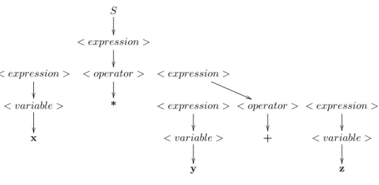
Starting with symbol S , we can easily create a complete derivation tree from this exam- ple grammar; as shown in Figure 2:

S < expression >

< expression >

< operator >

< expression >

(( < variable >

* < expression >

< operator >

< expression >

x < variable >

+ < variable >

y z

Figure 2: A GP “individual”, represented by a simple derivation tree.

Interestingly, there are two ways to interpret the “individual” in Figure 2. If you concen- trate on the derivation tree and follow its node expansions , then the sub-expression y+z merges up-tree into one node before the operator ∗ becomes active, and therefore y+z is to be calculated first. Hence, in this interpretation, the derivation tree represents the expression x*(y+z) . For maximum speed and efficiency, GP software implementations very often integrate the parsing process into the derivation tree, and then this is the result you get.

On the other hand, it is good software design practice to strictly separate software lay- ers. From this perspective, mixing the derivation tree and the parsing process is “messy”.

To ensure maximum modularity, it makes a lot of sense to clearly distinguish between the derivation tree (the so-called genotype ), and the resulting expression (the so-called phenotype ). In that case, the phenotype xy+z can be interpreted completely indepen- dent from its genotype* by a separate parser, and is - according to the common rule that multiplication has precedence before addition - to be interpreted as (x*y)+z . This is the approach taken by the software implementation discussed in this thesis.

It should be mentioned that there is an alternative approach to overcoming the encoding

problem mentioned at the end of Chapter 2. It is called Linear Genetic Programming

(LGP) and works without tree-representations under the condition that specific pro-

gramming languages are used. In this thesis we will not further investigate LGP.

(14)

3.2 Generating a Random Population, and the Depth Limit Problem

The first step in a GP algorithm is to generate a population of random individuals.

But even if you consider the very simple grammar as shown in Figure 1, it is obvious that because of the recursive nature of the grammar, an infinite amount of (ever larger) individuals can be derived from it.

Computing the exact number of individuals that can be generated in a certain number of steps from a given (maybe complex) grammar, and consequently computing the total number of individuals that can be generated for a maximum derivation depth limit, and doing so within a reasonable time frame, is in general a non-trivial task.

Luckily, although not entirely trivial, it is a task that has been already solved. In [Geyer-Schulz, 1994], an APL algorithm for calculating the number of individuals that can be derived in n steps for a given grammar was presented for the first time. Un- fortunately, the proposed implementation was too slow for most practical purposes. In [Hörner, 1996, p. 22-25], a much faster algorithm and its C++ implementation was presented, and is consequently also used in this work.

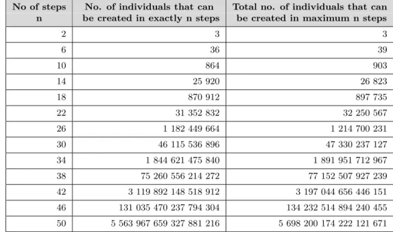
The following table is calculated by this algorithm, and shows how many individuals can be created in exactly n derivation steps, and also how many individuals can be created in total with a given maximum of n derivation steps from the sample grammar in Figure 1 (substitution of starting symbol S not included):

No of steps No. of individuals that can Total no. of individuals that can n be created in exactly n steps be created in maximum n steps

2 3 3

6 36 39

10 864 903

14 25 920 26 823

18 870 912 897 735

22 31 352 832 32 250 567

26 1 182 449 664 1 214 700 231

30 46 115 536 896 47 330 237 127

34 1 844 621 475 840 1 891 951 712 967

38 75 260 556 214 272 77 152 507 927 239

42 3 119 892 148 518 912 3 197 044 656 446 151

46 131 035 470 237 794 304 134 232 514 894 240 455

50 5 563 967 659 327 881 216 5 698 200 174 222 121 671

Table 1: Number of individuals that can be created from the sample grammar in Figure

1 in up to 50 derivation steps.

(15)

As the number of individuals that can be created is unlimited, one has to set an allowed maximum derivation depth. If you do so, the rightmost column of Table 1 gives you the sample size of all individuals that can possibly be created in n steps. That can be seen as the search space size .

If there is no hint which individuals are to be preferred, a natural strategy is to create an initial population where each individual of the search space has equal probability to be randomly created. In [Hörner, 1996, p 25-29], a time-efficient algorithm for achieving this task is presented, and it has been implemented by the author in the GPK software package used for this thesis.

However, if you look at the numbers in Table 1, you see that there are always over- whelmingly more individuals that can be created for your chosen maximum derivation depth n

max

than for all smaller derivation depths n < n

max

together. This is typical for all relevant grammars, and implies that, by choosing a maximum derivation depth n

_max

, you practically define the size of almost all individuals in the initial population.

This is a problem, as we usually don’t know the size of the solution we are looking for.

We will refer to how we approached this problem in Chapter 5.

3.3 Fitness Calculation and Fitness Scaling 3.3.1 Raw Fitness

The next step in any GP algorithm is to assign a raw fitness value f

_i^raw

to each individual i . This raw fitness value must give an indication on how “fit” the individual is with respect to the given problem. In our case, the mean square deviation between the values calculated by the individual’s phenotype and the measurement value data set is a good candidate for calculating f

_i^raw

. Actually, the mean square deviation is the basis for f

_i^raw

in our simulations, but also some “extras” have been added to calculating f

_i^raw

. We will elaborate the details in Chapter 4. Depending on the problem, f

_i^raw

is either to be maximized, or minimized. In our case, of course, it must be minimized.

3.3.2 Standardized Fitness

As the GPK software is for general use, and - depending on the task on hand - f

_i^std

must be either maximized or minimized, a so-called standardized fitness value f

_i^std

is calcu- lated for each individual i in the next step. As proposed by [Geyer-Schulz, 1994, p. 218], it is calculated differently for maximization tasks and minimization tasks, as to ensure that we get a fitness value where smaller values always indicate better individuals. For minimization tasks the standardized fitness is calculated as follows:

f

_i^std

= f

_i^raw

− min

i=1...n

f

_i^raw

(1)

(16)

where min

i=1...n

f

_i^raw

represents the smallest raw fitness value in the whole population at the time.

3.3.3 Adjusted Fitness

Next, the so-called adjusted fitness value f

_i^adj

is calculated for each individual i from f

_i^std

. It always has a value between 0 and 1, where larger values indicate fitter individuals. Any linear or non-linear function assigning larger values to fitter individuals which ensures that f

_i^adj

always lies between 0 and 1 is suitable. If the selection of individuals later is done proportional to the (normalized) fitness values (which are calculated from f

_i^adj

), this function influences the selection probability. It can be used, for example, to eliminate non-linearity of f

_i^raw

. In our implementation we have chosen the following function, as suggested by [Koza, 1992, p. 97]:

f

_i^adj

= 1

1 + f

_i^std

(2)

3.3.4 Normalized Fitness

Eventually, the normalized fitness value f

_i^norm

is calculated for each individual i accord- ing to [Geyer-Schulz, 1994, p. 218], so that the sum over all normalized fitness values equals 1:

f

_i^norm

= f

_i^adj

P

n

i=1

f

_i^adj

(3)

Again, the larger the value, the fitter the individual.

3.4 Inclusion of Sub-Trees

Consider the example derivation tree from Chapter 3.1, which produced the phenotype x*(y+z) . Maybe this phenotype has a rather bad fitness value. However, if we also consider all sub-trees starting with root-node <expression> , then we can additionally extract the following syntactically correct phenotypes from the derivation tree:

• x

• y+z

• y

• z

(17)

It is easily possible that some of these expressions have a better fitness than the complete phenotype x*(y+z) . Hence, it seems reasonable to also apply fitness values to some or all of these sub-expressions, and to create a “virtual” population that includes these additional phenotypes.

Because of this reasoning, the GPK software package offers the possibility to activate the inclusion of sub-trees with a defined minimum derivation size. However, multiple simulations run by the author indicated that permanent activation of this feature is not entirely beneficial and can lead to premature convergence. Therefore, in the actual simulations we only activated this feature once every 10 generational steps, which seemed to have a positive effect on the overall performance.

3.5 Selection

After calculating the fitness values for each individual in the population, a target sam- pling rate tsr

i

is to be calculated for each individual i. It gives the expected value for how often this individual i will be (on average) selected in the following random sampling process.

At first glance, calculating tsr

i

somehow proportional to f

_i^norm

seems reasonable, and it is indeed a method suggested by various authors (e.g. [Goldberg, 1989, p. 10ff], or [Schöneburg et al., 1994, p. 197ff]). However, this method has a serious drawback:

When the population is very diverse (e.g. at the beginning), the fittest individuals get a much higher chance of being selected than all others, and consequently tend to take over the whole population very soon. On the other hand, if (after a while) the population gets more and more homogeneous, the selection pressure drops, and the evolutionary process degrades to a mere random process.

To overcome these problems, [Grefenstette et al., 1989] suggested the method of Linear Rank Selection , and since then this method has been widely adopted in the GP commu- nity (see: [Poli et al., 2008, p. 32-34]). With this method, the target sampling rate tsr

_i

is calculated as follows:

tsr

_i

= tsr

_min

+ ( tsr

_max

− tsr

_min

) rank

_i

− 1

n − 1 (4)

where n is the total number of individuals in the population, rank

_i

is the rank of the i -th individual if ordered by f

_i^norm

in ascending order (starting with 1), and tsr

min

denotes the (chosen) target sampling rate for the unfittest individual. tsr

_max

must fulfill the following condition:

tsr

_max

= 2 − tsr

_min

(5)

(18)

3.6 Sampling

In the next step, a sample of individuals is to be drawn randomly in n drawings, where n denotes the size of the new population. In the simplest case of Stoachastic Sampling with Replacement the probability for the i -th inividual to be drawn is calculated by

p

i

= tsr

i

P

m

j=0

tsr

_j

(6)

where m denotes the number of individuals in the current population.

Of course, what can easily happen here, is that some individuals with a tsr around 1 have “bad luck” and are not sampled at all. To prevent this from happening, and to ensure maximal diversity, [Baker, 1987] suggested Stochastic Universal Sampling . That is the sampling method we have used in all our software simulations. The basic idea of Stochastic Universal Sampling is to sample all individuals in one drawing.

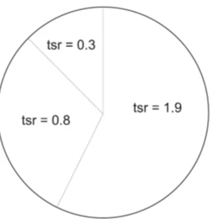
Let’s assume, for example, that we have a current population of size m = 3, and we want to sample 5 individuals ( n = 5). For the Stochastic Universal Sampling process, we can visualize a roulette wheel with 3 compartments, each sized according to the respective target sampling rate (see Figure 3).

Figure 3: “Roulette wheel” with 3 compartments, each sized according to the respective target sampling rate, from: [Hörner, 1996, p. 34].

For the actual sampling process, we put another wheel with n spokes on top of the first

one, and we spin it until it comes to a stop at a random position (see Figure 4).

(19)

Figure 4: Stochastic Universal Sampling of 5 individuals, from: [Hörner, 1996, p. 34].

In our example, as you can see from Figure 4, the sample consists of three copies of the individual with tsr = 1 . 9, and one copy of each for the other two individuals.

3.7 Mating

The next step in a GP algorithm is to find a mating partner for each individual in the previously generated sampling list. The mating method we have chosen for all of our simulations is Random Permutation Mating , as suggested by [Geyer-Schulz, 1994].

With this method, a random permutation of the previously generated sampling list is generated and assigned to the original list. Then, the i-th entry of the permutated list is the assigned mating partner of the i-th entry in the original list.

3.8 Cross-Over

For each pair in the mating-list there is a certain probability (chosen as a parameter for the simulation), that the following cross-over operator is applied (thereby generating a new population consisting of individuals forming - after applying some more genetic operators - the next generation):

• Count all tree-nodes representing non-terminal symbols (see Chapter 3.1) in the derivation-tree of the first mating partner.

• Select one of these nodes at random and remember the symbol.

• Find all tree-nodes of the second mating-partner having exactly the same symbol, and having a sub-tree small enough to potentially replace the sub-tree of the se- lected node in the first partner without exceeding the maximum derivation depth.

If no such node exists, repeat with step 1 until a maximum of 8 attempts have

been reached.

(20)

• Select one of the identified suitable nodes of the second mating-partner by random.

• Replace the sub-tree starting with the selected node of the first mating partner with the sub-tree starting with the selected node of the second mating partner.

If a pair is not chosen for cross-over, then the first mating partner is copied into the new population without any modification at that step.

3.9 Mutation

After mating and cross-over, mutation operators are usually applied in GP software.

There is an ongoing discussion to what extent mutation operators actually improve the performance of GP. [Luke and Spector, 1997] suggested that the performance gain due to mutation very much depends on the problem and the detail of the GP system.

Multiple mutation operators are described in literature (see [Poli et al., 2008, p.42-44], for example: Subtree Mutation, Size-Fair Subtree Mutation, Point Mutation, Hoist Mu- tation, Shrink Mutation, Permutation Mutation, Random Constant Mutation, or Sys- tematic Constant Mutation , to name just a few.

In our application we use Subtree Mutation , and Point Mutation , which are described in this chapter.

3.9.1 Subtree-Mutation

For each individual in the new population, which was created by mating and cross-over, there is a certain probability (chosen as a parameter for the simulation) that the subtree- mutation operator is applied.

The subtree-mutation operator simply replaces a randomly selected sub-tree (that’s any tree starting with a non-terminal symbol ) with a randomly generated sub-tree, while ensuring that the maximum derivation depth is not exceeded.

3.9.2 Point Mutation

After the tree-mutation operator has been applied, there is a certain probability (chosen as a parameter for the simulation) that the point mutation operator is applied.

From all terminal symbols of an individual’s derivation-tree the point mutation operator

chooses one at random, and replaces it with a randomly selected different terminal

symbol allowed by the grammar. One of the advantages of the point mutation operator

is that it helps evolving and fine-tuning number constants in the individual’s phenotype.

(21)

3.10 Elitism

The elitism-operator, if activated, is applied after all other operators. It ensures that there is always at least one copy of the previous generation’s best individual in the next generation of individuals.

3.11 Repetitive Application of all Genetic Operators

If all operators as described in Chapters 3.3 to 3.10 are applied to the initial random population, the first new (and hopefully fitter) generation has been created. After that, repetitive application of these operators lead to populations with ever fitter individuals, hopefully converging into an approximate or even exact solution to the given problem.

As described, there are a lot of parameters to be chosen, e.g. population size, maximum derivation depth, or various probabilities for cross-over and mutation operators, to name just a few. Choosing these parameters is an meta-optimization task in itself, and finding well-performing parameters often depends on the experience of the person running the simulations. It is also not uncommon to vary some of these parameters during the simulation process.

4 Software Structure

This chapter explains design and structure of the used software package. We hereby refer to the initial version of the software that was used in the first simulation round.

Any improvements that have been implemented in course of later simulation rounds are explained in Chapters 6.2 and 8.2.

The UML class diagram in Figure 5 shows the most relevant classes of both the Genetic Programming Kernel (that’s everything within the grey box), as well as of the software that has been implemented specifically for this thesis (that’s everything displayed above the grey box).

4.1 Genetic Programming Kernel

[Hörner, 1996] gives an extended description of the Genetic Programming Kernel (GPK).

As this thesis focuses on an GP application, using the GPK just as an tool, and as the general foundations of GP have been outlined in Chapter 3, a brief overview about what’s going on “under the GPK’s hood” should be sufficient here.

• Class Farm ist the GPK’s top class. It stores the population (or, optionally, several

populations, representing multiple generations), the grammar, and all simulation

parameters. Further, it gives top-level access to functions for configuring the simu-

lation parameters, like .SetFitnessScaling(...) , .SetTreeMutProb(...) , etc.,

and the .NextStep() function, triggering the next generational step.

(22)

(23)

• Class Language , of which an instance is stored in every instance of class Farm , is able to load a grammar from a grammar definition file, and provides access to all symbols and its derivations (with helper classes SymbTabEntry , which instances represent terminal- or non-terminal-symbols, and class ProdTabEntry , which in- stances represent derivations of non-terminal symbols). Further, class Language and its helper classes provide functions for search space size computing, as de- scribed in [Hörner, 1996].

• Instances of class Population represent a population of individuals in a specific generation. Further (if activated), this class generates a “virtual population”, in- cluding also all sub-trees down to a specified minimal derivation depth (see Chapter 3.4).

• Any instance of class RootNode , derived from class StartNode , represents a root node of a complete derivation tree.

• Any instance of class StartNode , derived from class TreeNode , represents a node of a derivation tree containing the grammar’s top-most non-terminal symbol (after the starting symbol S ). This class, for example, provides the public function for reading out a phenotype string.

• Eventually, any instance of class TreeNode represents any other node of a derivation tree. Of all the node-classes, this class contains most of the helper functions needed by the genetic operators, like “growing” a random tree, point mutation, and much more.

The pseudo number generator class Uniran is used by both the GPK itself, as well as by the newly developed class PhysModel . It is based on an PASCAL implementation described in [Law and Kelton, 2000, p. 428], and provides up to 255 independent pseudo random number streams.

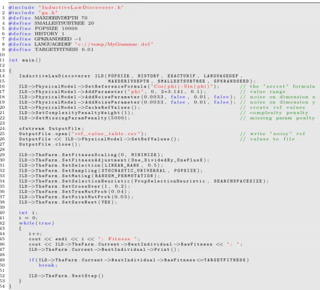
The following source code demonstrates how to use the “naked” GPK on top level, and

how to start a GP simulation in a few lines of code.

(24)

1 #i n c l u d e " ga . h "

2 #d e f i n e MAXDERIVDEPTH 70

3 #d e f i n e SMALLESTSUBTREE 20

4 #d e f i n e POPSIZE 1 0 0 0 0 5 #d e f i n e HISTORY 1 6 #d e f i n e GPKRANDSEED −1

7 #d e f i n e LANGUAGEDEF " c : / / temp /MyGrammar . d e f "

8 #d e f i n e TARGETFITNESS 0 . 0 1 9

10 i n t m a i n( ) 11

12 {

13 F a r m M a i n F a r m(P O P S I Z E, H I S T O R Y, E X A C T U N I F, L A N G U A G E D E F, M A X D E R I V D E P T H, 14 S M A L L E S T S U B T R E E, G P K R A N D S E E D) ;

15 M a i n F a r m.S e t F i t n e s s S c a l i n g( 0 , M I N I M I Z E) ;

16 M a i n F a r m.S e t F i t n e s s A d j u s t m e n t(O n e _ D i v i d e d B y _ O n e P l u s X) ; 17 M a i n F a r m.S e t S e l e c t i o n(L I N E A R _ R A N K, 0 . 5 ) ;

18 M a i n F a r m.S e t S a m p l i n g(S T O C H A S T I C _ U N I V E R S A L, P O P S I Z E) ; 19 M a i n F a r m.S e t M a t i n g(R A N D O M _ P E R M U T A T I O N) ;

20 M a i n F a r m.S e t S e l e c t i o n H e u r i s t i c(P r o p S e l e c t i o n H e u r i s t i c, S E A R C H S P A C E S I Z E) ; 21 M a i n F a r m.S e t C r o s s O v e r( 1 , 0 . 2 ) ;

22 M a i n F a r m.S e t T r e e M u t P r o b( 0 . 0 4 ) ; 23 M a i n F a r m.S e t P o i n t M u t P r o b( 0 . 0 3 ) ; 24 M a i n F a r m.S e t S a v e B e s t(Y E S) ; 25

26 i n t i;

27 i = 0 ; 28 w h i l e(t r u e)

29 {

30 i++;

31 c o u t << e n d l << i << " : F i t n e s s ";

32 c o u t << M a i n F a r m.C u r r e n t−>B e s t I n d i v i d u a l−>R a w F i t n e s s << " : "; 33 M a i n F a r m.C u r r e n t−>B e s t I n d i v i d u a l−>P r i n t( ) ;

34

35 i f(M a i n F a r m.C u r r e n t−>B e s t I n d i v i d u a l−>R a w F i t n e s s<=T A R G E T F I T N E S S)

36 b r e a k;

37

38 M a i n F a r m.N e x t S t e p( )

39 }

40 }

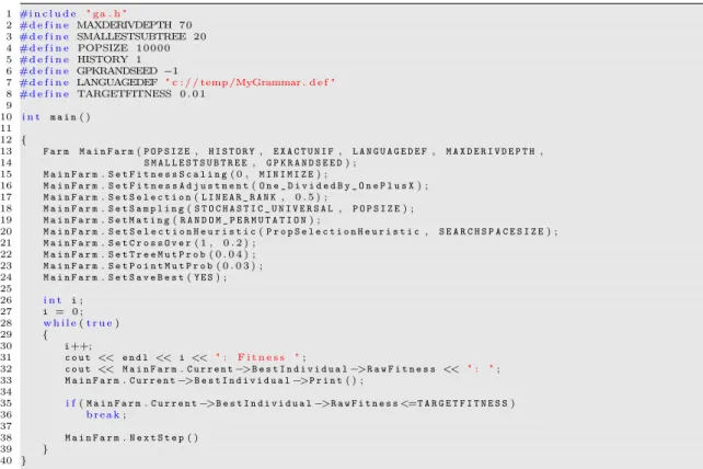
Figure 6: Sample source code, demonstrating how to use the “naked” GPK.

The above listing is easy to understand. In line 13, a new Farm is instanced, with POPSIZE 10000 individuals. HISTORY 1 means that genetic operators do not include previous generations, EXACTUNIF forces the GPK to create a uniformly distributed pop- ulation, and LANGDEF specifies from where to load the grammar definition file.

MAXDERIVDEPTH 70 limits the maximum derivation depth to 70 steps, SMALLESTSUBTREE 20 means that all sub-trees with minimum derivation depth of 20 steps should be in- cluded into the selection process. The last parameter GPKRANDSEED -1 is just the seeding value for the random number generator.

In lines 15-24, all other simulation parameters are defined. For example, line 15 de- fines that fitness scaling should only consider the current population (first parameter

= 0 ), and that the goal is to MINIMIZE the raw fitness (second parameter). Or, as

another example, line 21 defines that the cross-over parameter should do cross-over in

one point (first parameter), and be applied with a probability of 0.2 (second parameter).

(25)

Eventually, the main loop from line 28-39 prints out the currently best individual (and its fitness), and triggers the next generation (line 38). When the best individual is better than the desired target fitness, the loop is abandoned (lines 35 and 36).

However, there is one important topic that we have circumvented in this explanation so far: The above code will only work if we have added some code to evaluate the phenotypes, and to calculate the raw fitness value for each individual. This will be the subject of the next sub-chapters.

4.2 Mathematical Expression Parser “NumEval”

Any instance of NumEval is immediately able to evaluate BASIC-lime mathematical expressions. The expression must be passed by calling the function .Evaluate(string) , which returns the numerical value. If an error has occurred, .EvaluationOk() returns false , and .GetErrorCode() and .GetErrorMessage() provide further information about the problem. The parser works case-sensitive.

4.2.1 Mathematical Operators

The following common mathematical operators, considering the usual operator prece- dents, are included:

+, -, *, /, ^

The minus-sign can also act as an unary operator, reversing the sign of the expression on the right side.

4.2.2 Mathematical Functions

Further, the following common mathematical functions, all accepting exactly one pa- rameter, can be interpreted (where <num> stand for any syntactically correct numerical expression):

Sin(<num>), Cos(<num>), Tan(<num>), Abs(<num>), Exp(<num>), Log(<num>), ArcSin(<num>), ArcCos(<num>), ArcTan(<num>), Sinh(<num>), Cosh(<num>), Tanh(<num>), ArcSinh(<num>), ArcCosh(<num>), ArcTanh(<num>), Sqrt(<num>)

Also, a Min and a Max function has been included, both of which expect two numerical parameters:

Min(<num>, <num>), Max(<num>, <num>)

The numerical constant π is included as pseudo-function:

Pi()

(26)

4.2.3 Number Constants

Any string of digits with maximum one point in-between will be interpreted as number.

It is also possible to use numbers in scientific notation: Any number as defined before followed by an E , optionally followed by + or - , and then followed by one or two further digits will be interpreted as a number in scientific notation.

4.2.4 Boolean Operators

The NumEval class is also able to handle boolean algebra. The numerical value 0 is in- terpreted as false , and any other numerical value as true . These are the implemented boolean operators, acting on the boolean value on the left and the right side, and re- turning a boolean value:

And, Or, Xor

The “Not” operator is implemented as function, accepting exactly one (boolean) value:

Not(<bool>)

4.2.5 Comparison Operators

The following comparison operators, comparing the numerical value on the left and on the right side, and returning a boolean value, are also implemented:

<, >, >=, <=, <>, =

This allows for the implementation of an Iif -function, which expects three parameters:

One boolean, and two numerical:

Iif(<bool>, <num>, <num>)

4.2.6 Variables

As the GP algorithm should eventually produce mathematical functions, which necessar-

ily depend on one or more variables, the NumEval class must be able to also interpret these

variables (like, for example t , for time). Therefore, it can be initialized with two func-

tion pointers of type bool IsParameter(string) and double e_Parameter(string) .

These functions must be provided externally (in our case they are provided from class

PhysModel ). Whenever the parsing algorithm comes across a potential variable, it first

calls IsParameter(string) to find out, whether this is a valid variable at all. If yes,

e_Parameter(string) is called to fetch the current value of this variable.

(27)

4.2.7 Complexity

After having evaluated a formula, the public integer variable .Complexity provides in- formation about the function’s complexity. This is how this value is calculated:

It comes naturally that the parser works recursively. Every time the internal parsing function .e_prs(string) is called recursively, the value of .Complexity is increased by one. So, for example, while evaluating the expression

Sin(Sqrt(t+2))

the parsing function is called five times:

• .e_prs("Sin(Sqrt(t+2))")

• .e_prs("Sqrt(t+2)")

• .e_prs("t+2")

• .e_prs("t")

• .e_prs("2")

Hence, the expression Sin(Sqrt(t+2)) has a .Complexity value of 5.

4.3 Physical System Simulator “PhysModel”

4.3.1 User Functions

An instance of class PhysModel represents the to-be-discovered physical system. First of all, it stores the “secret” formula, which represents the system. This formula can be set with .SetReferenceFormula(string) . The formula can have one or more vari- ables, and it can represent both a scalar or an vector. For the latter, simply multiple expressions are concatenated with an “ : ”. For example, "Cos(phi):Sin(phi)" would represent an unit circle in polar coordinates.

Then, all valid parameters (variables), plus their value ranges, plus the step-width for

the to-be-generated value list must be defined. This is done by means the function

.AddParameter(...) . In our unit circle example, we could set the parameter ϕ to run

from 0 to 2π in steps of 0.1 by calling .AddParameter("phi", 0, 2*3.141, 0.1) .

Optionally, it can be defined if (and if yes, how much) Gaussian random noise (sim-

ulating measurement errors) should be superimposed on the values. This is done by

calling the function .AddNoiseParam(..) , which accepts 4 parameters. The first pa-

rameter double Sigma is the sigma value for the Gaussian distribution. The sec-

ond value bool SigmaAbsolute defines, how Gaussian distributed random numbers

(28)

GaussRnd( Sigma ) are superimposed on the simulated measurement values v . If SigmaAbsolute == true , then the random number is added as follows:

v

_noisy

= v + GaussRnd( Sigma ) (7)

If SigmaAbsolute == false , then the “noisy” value v

noisy

is calculated this way:

v

noisy

= v · (1 + GaussRnd(Sigma)) (8)

The last two parameters are double Tolerance and bool .ToleranceAbsolute . If during the calculation of the mean square deviation over all reference values the differ- ence between a (noisy) reference value and the to-be-tested function is smaller than the Tolerance value, then for this point a deviation of zero is assumed. The ToleranceAbsolute parameter defines, whether the Tolerance value is meant as an absolute value, or as an relative tolerance.

After having defined the system, the reference value list is generated by calling .CacheRefValues() . The function .GetRefValues() can be used to export the whole reference value table (including all noisy values) in CSV format.

4.3.2 Internal Relations

On one hand, class PhysModel instances and internally uses class NumEval for initially calculating the reference value list, and for calculating mean square deviation values during the simulation. To enable class NumEval to parse expression with variables (“pa- rameters”), is provides to the instance of class NumEval the required information about parameter values (see Chapter 4.2.6).

On the other hand, class PhysModel is instanced and managed by class InductiveLawDiscoverer , which is the top-level class of our simulation package (in its initial version), and connects the instances of PhysModel and Farm .

4.4 Top-Level Class InductiveLawDiscoverer

First of all, class InductiveLawDiscoverer provides the implementation for calculating the respective raw fitness values (function .RawFitnessFunction(string) ). When in- stancing class Farm , it passes to the instance of Farm a function pointer to .RawFitnessFunction(string) , so that every time an individual needs to get an raw fitness value assigned, it can fetch this value from InductiveLawDiscoverer .

To be able to provide this value, InductiveLawDiscoverer also instances class PhysModel ,

(29)

4.4.1 Raw Fitness Calculation

In order to calculate the raw fitness of an expression, the InductiveLawDiscoverer class calls PhysMode.GetResidualSquareSum() , thereby calculating the mean quadratic de- viation over all reference points by (under consideration of the tolerance levels for noisy values, see Chapter 4.3.1).

With vectorial expressions (e.g., the orbit of a planet in cartesian coordinates), several expressions are generated from the grammar (one for each dimension of the vector). The basis for the raw fitness is then simply the mean square deviation over all expressions.

Hence, the mean square deviation m for a D-dimensional expression v( d, t ) that, for example, depends in each dimension d solely on time t , is calculated over the time interval t

min

...t

max

with step width s as follows:

m = 1

n

D

X

d=1

(tmax−tmin)/s

X

j=0

(v

ref

( d, t

_min

+ ( t

_max

− t

_min

) js ) − v ( d, t

_min

+ ( t

_max

− t

_min

) js ))

²

(9) where v

ref

( d, t ) denotes the reference value for dimension d and at time t , and v( d, t ) denotes the value of the to-be-tested function for dimension d and at time t .

Optionally, the following penalties are added to the mean square deviation:

• P

const

: A configurable penalty value by which the mean square deviation value is increased if the expression is merely a constant; that is, if the parameters (e.g., time t or the path angle ϕ ) do not occur in the generated expression. For multi- dimensional expressions, P

const

is added, even if only one expression of the vector is a constant.

• P

complexity

: A configurable penalty value that is multiplied with the expression’s complexity as calculated by NumEval.Complexity (see Chapter 4.2.7).

• If the attempt to compute the numerical value of an expression does not result into a real value for all of the reference points (for example because at one point it results in a division by zero or because of the attempt to calculate the root of a negative number), then the “worst possible” fitness value 1 . 7 · 10

³⁰⁸

is assigned.

Hence, the raw fitness value f

_i^raw

for a D-dimensional expression that depends solely on the time t , is calculated as follows:

f

_i^raw

=

( m + P

_const

+ P

_complexity

. . . m ∈ R

1.7 · 10

³⁰⁸

. . . ..m / ∈ R (10)

(30)

4.4.2 Using the Whole Software Package via InductiveLawDiscoverer

The source code in Figure 7 gives an example on how to use the whole software package via the top-level class InductiveLawDiscoverer .

It is easy to see that this code example looks almost exactly like the example in Chapter 4.1. There are just two differences:

The Farm is now instanced by and accessed via the InductiveLawDiscoverer instance ILD , and - most importantly - using the functions described in the previous sub-chapters, it is now possible to define in lines 16-22 the to-be-discovered system (here: a simple system describing a unit cycle parametrized by the angle ϕ ).

Automated Generation of Physical Theories by a Genetic Programming Algorithm

Helmut Hörner