Schriften aus der Fakultät Wirtschaftsinformatik und
Angewandte Informatik der Otto-Friedrich-Universität Bamberg
24
Udo R. Krieger, Thomas C. Schmidt, Andreas Timm-Giel (eds.)
MMBnet 2017
Proceedings of the 9th GI/ITG Workshop
„Leistungs-, Verlässlichkeits- und Zuverlässigkeitsbewertung
von Kommunikationsnetzen und Verteilten Systemen“
Schriften aus der Fakultät Wirtschaftsinformatik und Angewandte Informatik der Otto-Friedrich- Universität Bamberg
24
Contributions of the Faculty Information Systems and Applied Computer Sciences of the
Otto-Friedrich-University Bamberg
und Angewandte Informatik der Otto-Friedrich- Universität Bamberg
Band 24
2017
Contributions of the Faculty Information Systems and Applied Computer Sciences of the
Otto-Friedrich-University Bamberg
MMBnet 2017
Proceedings of the 9 th GI/ITG Workshop
„Leistungs-, Verlässlichkeits- und Zuverlässigkeitsbewertung von Kommunikationsnetzen und Verteilten Systemen”
Udo R. Krieger, Thomas C. Schmidt, Andreas Timm-Giel (eds.)
University of Bamberg Press
2017
Dieses Werk ist als freie Onlineversion über den Hochschulschriften-Server (OPUS; http://
www.opus-bayern.de/uni-bamberg/) der Universitätsbibliothek Bamberg erreichbar. Kopi- en und Ausdrucke dürfen nur zum privaten und sonstigen eigenen Gebrauch angefertigt werden.
Herstellung und Druck: Digital Print Group, Nürnberg
Umschlaggestaltung: University of Bamberg Press, Larissa Günther Umschlagbild: © Marcel Großmann
© University of Bamberg Press Bamberg, 2017 http://www.uni-bamberg.de/ubp/
ISSN: 1867-7401
ISBN: 978-3-86309-501-7 (Druckausgabe) eISBN: 978-3-86309-502-4 (Online-Ausgabe) URN: urn:nbn:de:bvb:473-opus4-497624 DOI: http://dx.doi.org/10.20378/irbo-49762
Die Deutsche Nationalbibliothek verzeichnet diese Publikation in der
Deutschen Nationalbibliographie; detaillierte bibliographische Informationen sind im
Internet über http://dnb.d-nb.de/ abrufbar.
Contents
Organization III
Invited Talk 1
Caching for Content Delivery and Cloud Services
Gerhard Haßlinger . . . . 3
Workshop Papers 1
Real-Time Communication 3
Saving Bandwidth by Limiting the Buffer Size in HTTP Adaptive Stream- ing
Sebastian Surminski, Christian Moldovan, Tobias Hoßfeld . . . . 5 On the Probability of Meeting Deadlines in IP-based Real-time Commu-
nication
Alexander Beifuß . . . . 23
New Network and Application Architectures 43
Combining Satellite and Terrestrial Communication Systems: Introduc- tion of the Transparent Multichannel IPv6 (TMC-IPv6) Project
Jörg Deutschmann, Kai-Steffen Hielscher, Reinhard German . . . . 45 Evaluation of Actor Based Code Offloading from Android Smartphones
in Real-Time
Marcel Großmann, Andreas Keiper . . . . 61
Author Index 81
Organization
The 9 th GI/ITG Workshop MMBnet 2017 „Leistungs-, Verlässlichkeits- und Zu- verlässigkeitsbewertung von Kommunikationsnetzen und Verteilten Systemen”
was organized by the Institute of Communication Networks at Hamburg Univer- sity of Technology (TUHH), the Internet Technologies Group at Hamburg Univer-sity of Applied Sciences (HAW Hamburg) and the Faculty of Information Systems and Applied Computer Sciences, Professorship of Computer Science, on behalf of University of Bamberg, Germany.
Organizing Committee General Chairs
Udo R. Krieger University of Bamberg, Germany
Thomas C. Schmidt Hamburg University of Applied Sciences (HAW Hamburg), Germany
Andreas Timm-Giel Hamburg University of Technology (TUHH), Germany
Technical Program Committee
Torsten Braun Universität Bern
Peter Buchholz TU Dortmund
Georg Carle TU München
Hans Daduna Universität Hamburg Hermann De Meer Universität Passau
Markus Fidler Leibniz Universität Hannover
Reinhard German Friedrich-Alexander Universität Erlangen- Nürnberg
Gerhard Haßlinger Deutsche Telekom AG and TU Darmstadt Klaus-D. Heidtmann Universität Hamburg
Tobias Hoßfeld Universität Duisburg-Essen Udo R. Krieger Universität Bamberg
Paul J. Kühn Universität Stuttgart Michael Menth Universität Tübingen Peter Reichl Universität Wien
Johannes Riedl SIEMENS AG
Thomas C. Schmidt HAW Hamburg Jens B. Schmitt TU Kaiserslautern
Markus Siegle Universität der Bundeswehr München
Otto Spaniol RWTH Aachen
Dirk Staehle Hochschule Konstanz – Technik, Wirtschaft und Gestaltung
Helena Szczerbicka Leibniz Universität Hannover Andreas Timm-Giel TU Hamburg-Harburg
Kurt Tutschku Blekinge Institute of Technology, Karlskrona
Tadeus Uhl Hochschule Flensburg
Alexander von Bodisco Hochschule Augsburg
Oliver Waldhorst Hochschule Karlsruhe - Technik und Wirtschaft Bernd E.Wolfinger Universität Hamburg
Martina Zitterbart KIT Karlsruhe
Additional Reviewer
Gerhard Haßlinger Deutsche Telekom AG and TU Darmstadt
Preface
Today, the demand for smart, efficient services and the effective transport of their related traffic streams is rapidly increasing on a global scale. It is arising from growing mobility, new industrial services, smart cities, complex private applica- tions, and the dissemination of multimedia information. The latter is caused by underlying massive human interactions and supported by a variety of online social networks. The integration of wireless 5G networks, wired high-speed networks and the evolving Internet-of-Things additionally provides major drivers of the fast growing Internet traffic. The steadily increasing demand to utilize the deployed network infrastructures and server resources most effectively generate some of the greatest challenges for engineering and science in modern information societies.
Mathematical methods of systems and network monitoring, modeling, simula- tion, and performance, dependability and reliability analysis constitute the founda- tion of modern quantitative evaluation methods. These techniques represent the basis for an application of the underlying methodologies to a large variety of areas in modern information society. If we consider the mathematical and technical foundation of currently applied modeling, analysis, simulation, and performance evaluation techniques with regard to their future development, a substantial scien- tific training and a constructive dialog of young scientists and upcoming engineers with experts in the field is needed. It may facilitate a more efficient way to apply these new techniques and reveal the most effective modalities to design software- defined next-generation networks and advanced cloud computing systems of an information society.
To support the sketched personal development goals of young scientists and
engineers working in this area, the responsible administrative forum of GI/ITG
Technical Committee “Measurement, Modelling and Evaluation of Computing
Systems” (MMB) has established the workshop series MMBnet. The MMB com-
munity hopes that related research activities of young members can be stimulated by these means. Covering corresponding research topics of MMB, the 9 th GI/ITG Workshop MMBnet 2017 „Leistungs-, Verlässlichkeits- und Zuverlässigkeitsbe- wertung von Kommunikationsnetzen und Verteilten Systemen” was held at Hamburg University of Technology (TUHH), Germany, on September 14, 2017.
After a careful review process, the Organizing Committee of the workshop has compiled a scientific program that included 4 regular papers and the invited talk
“Caching for Content Delivery and Cloud Services: Use Cases, Caching Strategies and Performance Evaluation” by Dr. Gerhard Haßlinger, Deutsche Telekom AG and TU Darmstadt, Germany. We thank the authors for their submitted papers and all speakers, in particular the invited expert, for their lively presentations and the constructive discussions.
As conference chairs we are grateful for the support of all members of the Tech- nical Program Committee and we also thank the external reviewer for his dedi- cated service and for the timely provision of the reviews.
We express our gratitude to Hamburg University of Technology as conference host of MMBnet 2017 and, in particular, to all members of the local organizers’
team regarding their great efforts.
We acknowledge the support of the EasyChair conference system and express our gratitude to its management team.
Last but not least, we appreciate the relentless support by Marcel Großmann, Faculty WIAI at University of Bamberg, and University of Bamberg Press while compiling the proceedings.
Finally, we hope that our reader’s future research on monitoring, modeling, analysis, and performance evaluation of next-generation networks and distributed systems will benefit from the proceedings of the 9 th GI/ITG Workshop MMBnet 2017.
September 2017
Udo R. Krieger
Thomas C. Schmidt
Andreas Timm-Giel
Invited Talk
Caching for Content Delivery and Cloud Services: Use Cases, Caching Strategies and Performance Evaluation
Gerhard Haßlinger
Technische Universität Darmstadt and Deutsche Telekom AG
Heinrich-Hertz-Straße 3-7 D-64295 Darmstadt, Germany
Abstract
The topic of Internet content caching regained relevance over the last decade due to the extended use of data center infrastructures in CDNs, clouds and ISP networks to meet capacity and delay demands of multimedia services.
The talk addresses global CDN and cloud platforms from QoS demands to the underlying server and caching architectures as well as statistics on the traffic and user request behavior.
Appropriate caching strategies have to be assessed in a tradeoff between hit rate efficiency and simple cache update processes. Results on the cache hit rate are presented comparing three types of cache (replacement
1) strategies based on
– LRU: Least Recently Used, – LFU: Least Frequently Used,
– Optimum caching with knowledge of future requests.
Caching evaluation results are obtained by simulation on the entire range of Zipf distributed user requests, which have been confirmed for many web applications.
Analytic results are also relevant for special cases. Optimum caching turns out to provide a non-trivial playground for Markov models. Finally, we show that opti- mum caching does not only provide a theoretical upper bound on the hit rate, but can be combined for improving usual strategies whenever a limited look-ahead is possible.
1
Web caches can also select their input in contrast to paging systems and local caches.
Curriculum Vitae
Gerhard Haßlinger has more than 10 years of experience as a researcher and
lecturer in computer science at Darmstadt University of Technology, and as an
engineer at Deutsche Telekom, where he works on architectures for service and
Internet access provisioning via fixed/mobile broadband platforms. His research
interests include content distribution, traffic engineering, reliability, and quality
of service aspects of computer and communication networks, information theory
and coding.
Workshop Papers
Real-Time Communication
Saving Bandwidth by Limiting the Buffer Size in HTTP 6daptive Streaming
Sebastian Surminski, Christian Moldovan, Tobias Hoßfeld University of Duisburg-Essen
http://www.uni-due.de
6bstract. Video streaming is one of the most bandwidth-intensive ap- plications on the Internet. In HTTP adaptive video streaming the video quality is selected according to the available bandwidth. To compen- sate bandwidth fluctuations, players use a buffer in order to ensure a smooth video output. On one hand, if the buffer runs empty, the video playback stops, which users experience as negative. On the other hand, if the user aborts video playback, the video in the buffer was unneces- sarily transmitted, hence this bandwidth was wasted. In this paper, we present a study in which we investigate the behavior of two video players and different buffer configurations in real-world bandwidth scenarios.
Thereby, we focus on the dimensioning of the buffer size and the trade- off between wasted bandwidth and the playback quality.
Key words: Buffer, Adaptive Video Streaming, Wasted Bandwidth
Introduction
Video streaming is a popular service on the Internet. It accounts for about 70%
of all downstream traffic on fixed access networks in North America during peak evening hours [1]. As a consequence, it is worth investigation and identification of saving potentials by limiting unnecessary transmissions. Nowadays, mainly HTTP adaptive streaming (HAS) is used. This means, that the video is played while being downloaded, and the video quality is selected according to the avail- able bandwidth. As this process is sensitive regarding bandwidth degradations and especially outages, the player maintains a buffer of video that is yet to be played, to cope with bandwidth fluctuation. This happens mainly while being on the move.
If the buffer runs empty, because the video is played faster than downloaded, the
playback stops. From user studies, it is known that such stalling events have a negative impact on the Quality of Experience (QoE) [2].
On the downside, video playback is often aborted by the user before the video has been completely played. This means that the remaining content of the buffer is never played, hence transmitted without need, which means this bandwidth is wasted. A study on YouTube in 2011 showed that about 60% of all requested videos were watched for less than 20% of their duration. In numbers, about 40% of all viewed videos on YouTube were aborted within the first 30 s, 20% of the videos were played less than 10 s [3].
Considering these facts, it is interesting to investigate the influence of the buffer size on the playback behavior of HAS video players, under realistic bandwidth conditions in mobile scenarios. To do so, we conducted a measurement study in which we evaluated the playback behavior of two different HAS video players in real-world scenarios. Subject to this study are two different video players, namely the YouTube player
1and the Shaka player
2. The Shaka player allows us to configure the buffer configuration, this way we can compare different buffer configurations.
The bandwidth conditions, that the players face, are mobile scenarios, which were recorded in everyday commuting situations, using different means of transport.
This methodology allows investigating the behavior of video players, especially the adaptation logic. Additionally, we have developed a method to evaluate the buffer level of the video player. By this, we can determine the amount of video that is wasted when playback of the video is aborted.
The structure of this paper is as follows. First, we introduce the issue of wasted bandwidth and its implications, as well as previous work on this topic in Section 2. After that, we sketch the way HAS works and the influence of the buffer size. In Section 3, we describe the methodology of the experiments we conducted. In Sec- tion 4, the results are presented. The paper ends with the conclusions in Section 5.
1
https://www.youtube.com
2
https://github.com/google/shaka-player
Background and Related Work
First, we identify the causes for wasted bandwidth. Then we introduce basic con- cepts of HAS. Different aspects of the buffer size in HAS were investigated in previous work, which we will present in the final part of this section.
. Wasted Bandwidth
For video streaming services, wasted bandwidth at large scale induces significant costs. Not only server capacities, but also link capacity is unnecessarily used. The implied cost is not only relevant for the video provider, but also for the user, for example when the user is on a data plan. There, often a fixed, maximum data contingent is determined. Additional traffic costs extra charge. So the user is in- terested in saving bandwidth, in the best case without reducing the video quality [4]. Additionally, transmitting data consumes a lot of energy on mobile devices.
Thus, transmitting less data may increase battery life time [5].
Furthermore, wireless networks have a limited overall capacity per cell. So it is interesting to limit the traffic transmitted to allow to serve more users per cell, and improve the overall performance of all users.
. 6daptive Video Streaming
Adaptive video streaming allows to adapt the video quality to the available band- width using different quality levels. To do so, the video is encoded in different qual- ities, the so-called representation levels, which are then split into small segments, typically with a length of several seconds. The video player selects autonomously which segments to play. Optimally, the video player selects the maximum quality without exceeding the available bandwidth. On one hand, if the player is too con- servative, the video quality is not as good as it could be. On the other hand, if the bandwidth is exceeded, the video is played faster than it is possible to fetch new video data. However, the player has to select the right quality level depending on the current available bandwidth.
. Buffer Size
To compensate for bandwidth fluctuations, the player maintains a playback buffer.
In this work, we measure the buffer level by the length of the video it contains,
independently of the actual file size. If the buffer runs empty, the playback stops.
This is called a stalling event. Users experience stalling events as very negative, so they have to be prevented [6]. The playback is resumed if the buffer is sufficiently filled. In the following, this limit is called the rebuffering goal. The maximum fill level of the buffer is called the buffer size.
When speaking about the buffer size, we simplify it by referring to the length of the video in the buffer, not the file size of the video. This is the same way it is done by video players like the Shaka player, which we use in this study, and also in research investigating this topic, like [16]. From the perspective of wasted bandwidth, it would make more sense to determine the buffer level depending the file size. Using the average video data rate, which can be found in Section3.5, an estimation of the wasted bandwidth can be done from the buffer level.
. Related Work
Research on HAS often focuses on the adaptation strategies, which select the rep- resentation layer, e.g. the segments that will be played. Especially in mobile scenar- ios, the available bandwidth is constantly changing. As this development is diffi- cult to foresee, the adaptation logic is limited, although there are good approaches, like [7]. To solve this problem, location-aware approaches have been introduced.
This allows to predict the bandwidth in the future and to adapt the video qual- ity accordingly. On one hand, this approach is appealing because it allows better adaptation of the video quality, and in practice, mobile devices already come with technology to determine their location. On the other hand, this introduces techni- cal overhead and serious privacy concerns [8], [9].
Nevertheless, the issue of wasted bandwidth has already been addressed by re- search from different points of view. Li et al. addressed the aspect of energy con- sumption and introduced a cache management method that reduces the power consumption of the radio modules in smart phones [10], [11]. Wu et al. presented an adaptive method to reduce the amount of wasted bandwidth by making the buffer size of HAS players adaptive [12]. This approach allows to weigh the costs for transmitting data and its energy consumption and react accordingly.
In this paper, we conduct experiments with HAS video players. To do so, we
use the players’ API to monitor the behavior and the internal status, including the
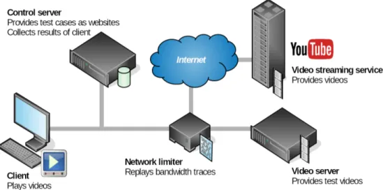
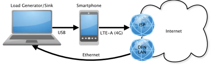
Fig. 1. Overview of the setup of our experiment. The client is directly connected to the control server, while the video is transmitted via the network limiter.
buffer level. Another approach for monitoring video players is made in [13], where the video playback is monitored using an Android application. Both methods need cooperation with the users or the video server. A completely passive monitoring technique is presented in [14] with the tool YOUQMON. Instead of monitoring the video player directly, the data stream is captured. With this information the supposed behavior of the player is simulated, which allows to predict when stalling events occur.
Methodology
We developed a setup that allows us to test HTML video players under predefined bandwidth conditions, while monitoring their behavior. In the experiments, we used two different video players for HAS. Our complete setup is shown in Figure 1. In the following, we describe the elements of our setup.
. Video Players
For the experiments, we used two different video players. The YouTube player is used by the most popular video streaming web site YouTube. So it represents the state of the art for HAS, that is used in practice. We compare it to the Shaka player, an open source video player, that allows us to configure the buffer configuration.
This way, we can change the buffer configuration and investigate its effects on the
playback behavior.
Both video players offer a JavaScript API to control and give status information.
Our approach is to use these interfaces to monitor the playback behavior to get statistics about the video playback. As these numbers are directly taken from the video player, they are very accurate. While the YouTube player has to be treated as a black box, the open source player can be configured, so it is possible to change its buffer configuration, in particular, the buffer size and the rebuffering goal. The buffer size is the maximum length of the video, that can be stored in the buffer.
The rebuffering goal defines the minimum buffer level, which needs to be reached, before the player starts playing the video. This is relevant, as a lower buffer level can reduce the stalling time, but increase the stalling frequency, which both have an influence on the QoE.
Using the players’ API, we collected the following information, which then was used to determine the quality of the playback of the video:
– Initial waiting time
– Number and duration of stalling events – Resolution of the video and adaptation events – Buffer level
Additionally, we also documented the bandwidth of the video stream and the band- width estimation of the player.
. Client
The client can be an arbitrary device running a recent web browser, that is able to run the video player. In our experiments this is a Firefox 50 browser on a machine running Ubuntu 16.04. It could also be changed to any other device, for example a smart phone, to investigate whether the players behave differently on other device types.
. Control Server
The experiment is controlled by the ‘Control server’, which provides the web page
for the client with the video player, and collects the results. In case of the Shaka
player, the video is hosted using a local video server. With the YouTube player,
we had to use YouTube as video source. Because of this, we had two differently
encoded versions of the same video. This is further described in Section 3.5.
. Network Limiter
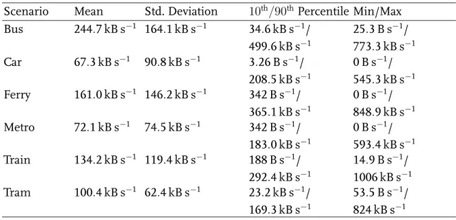
The bandwidth is controlled by bandwidth traces, which reflect real-world scenar- ios. These were provided by Riiser et al. using a notebook and a 3G modem for measuring download speed, and a GPS module for localization [15]. The team in- vestigated bandwidth rates on different mobile travel situations. During the mea- surements, files were downloaded via HTTP constantly. As this is the same tech- nique used by adaptive video streaming the same behavior would be experienced by a video streaming client. The bandwidth traces reflect situations as they are typ- ical for commuting, using different ways of transportation (bus, car, ferry, metro, tram, and train). We focus on mobile scenarios, because in these the bandwidth is varying, while in stationary situations, there is often more bandwidth available, which also has a lower variation over time. Numbers about the bandwidth sce- narios can be found in Table 1. These bandwidth traces are reproduced using tc
3which configures the packet scheduler of the Linux kernel of a dedicated Linux machine.
Table 1. Bandwidth characteristics of the bandwidth traces.
Scenario Mean Std. Deviation 10
th/90
thPercentile Min/Max Bus 244 . 7 kB s
−1164 . 1 kB s
−134 . 6 kB s
−1/
499.6 kB s
−125 . 3 B s
−1/ 773.3 kB s
−1Car 67 . 3 kB s
−190 . 8 kB s
−13 . 26 B s
−1/
208.5 kB s
−10 B s
−1/ 545.3 kB s
−1Ferry 161 . 0 kB s
−1146 . 2 kB s
−1342 B s
−1/
365 . 1 kB s
−10 B s
−1/ 848 . 9 kB s
−1Metro 72 . 1 kB s
−174 . 5 kB s
−1342 B s
−1/
183.0 kB s
−10 B s
−1/ 593.4 kB s
−1Train 134 . 2 kB s
−1119 . 4 kB s
−1188 B s
−1/
292 . 4 kB s
−114 . 9 B s
−1/ 1006 kB s
−1Tram 100 . 4 kB s
−162 . 4 kB s
−123 . 2 kB s
−1/
169 . 3 kB s
−153 . 5 B s
−1/ 824 kB s
−1. Video Server
The video players use different video sources. While the video source of the Shaka player can be configured arbitrarily, the YouTube player can only play videos from
3
http://manpages.ubuntu.com/manpages/xenial/en/man8/tc.8.html
Trace 1 Trace 2
...
Trace 1 Movie
Trace n
Transmission
Movie Transmission
Movie Transmission
Movie Transmission
Movie Transmission
Movie Transmission
Fig. 2. Repetition of bandwidth traces and videos. When the movie finished play- ing, the playback statistics are sent to the control server. After that, the movie is played again.
YouTube. As a result, we had to use different test videos. The video for the Shaka player was provided by a local web server. The YouTube player fetched a video di- rectly from YouTube. Because this relies on an Internet connection, during the experiments the Internet connectivity was continuously monitored to detect im- pairments.
Both video players used the same test movie with a length of 9 min 54 s, but in a different encoding and different representation layers. While the video for the Shaka player comes with three quality (Average data rate 79 . 99 kB s
−1, 178 . 60 kB s
−1, 482 . 69 kB s
−1) levels, the YouTube video has seven quality levels (Average data rate 13 . 41 kB s
−1, 30 . 17 kB s
−1, 40 . 70 kB s
−1, 80 . 08 kB s
−1, 150 . 60 kB s
−1, and 268 . 72 kB s
−1).
This means the YouTube player has a lower minimum and maximum bandwidth and more possibilities to adapt the video quality to the current available bandwidth.
. Mode of Operation
The mode of operation is as follows: The bandwidth traces of one scenario are
infinitely repeated by the bandwidth limiter. At the same time, the video playback
is repeated continuously, so that it starts at different positions of the bandwidth
traces. This process is also shown in Figure 2. Using the players’ API, every second
the current playback status, the buffer level and video quality are recorded, which
are then sent to the control server after a video playback has finished. Additionally,
this is also done whenever a stalling or adaptation event occurs. This way, we obtain
a precise history of the players’ behavior.
Results
In this Section, we present the results of the experiments. Each experiment can be identified by two different parameters: the video player (either YouTube player or Shaka player) and the bandwidth scenario (Bus, Car, Ferry, Metro, Train, Tram or Unlimited). The bandwidth scenario determines the precise available bandwidth at every time. In case of the Shaka player, also the buffer configuration can be changed. Then, the rebuffering goal and the buffer size can be configured, both parameters are explained in Section 2.3. The video player plays the test video. All experiments use the same test video, but the two different players use a different version of it.
. Shaka Player
With the Shaka player, we conducted experiments with different buffer configu- rations. The rebuffering goal sets the lower threshold when the playback starts, and the buffer size determines the maximum amount of video in the buffer. As all experiments are run in real-time, we limited the experiments to four different configurations: the default values with a buffer size of ten and a rebuffering goal of two seconds, a rebuffering goal of ten seconds, together with an increased buffer size of 90 and 180 seconds, and finally a high rebuffering goal of 20 seconds and 180 seconds buffer size.
Played Resolution and 6daptation Events In Figure 3, the number of adaptation events per video is plotted. An adaptation event means that the player changes the playback quality, thus selects another representation layer.
The number of adaptation events clearly differs between the different bandwidth traces. The bandwidth scenarios with the highest numbers of adaptation events are
‘Bus’, ‘Ferry’, and ‘Train’ with a median number of adaptation events between five
and six, respectively three and four, and two in case of ‘Train’. Those bandwidth
scenarios are the three with the highest average bandwidth, and play a signifi-
cant share of the video in medium quality, while in all other scenarios nearly all
the time the lowest quality is played. As it can be expected, with unlimited band-
width, always one single adaptation event occurs, when the player switches from
the initial quality to the highest representation layer. It is notable, that the buffer
configuration has no influence on the number of adaptation events.
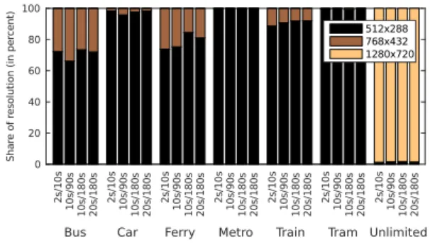
Figure 4 shows the distribution of the resolutions, in which the video was played.
In case of unlimited bandwidth, most of the time the video was played at maxi- mum quality. When the bandwidth was limited, the highest quality was never played, most time the lowest quality was selected. Only in the scenarios ‘Bus’,
‘Ferry’, and ‘Train’ the medium quality was played for a significant time. It can be assumed, that only in these scenarios the bandwidth was high enough, see Table 1.
0 5 10 15
Number of adaptation event 2s/10s 10s/90s 10s/180s 20s/180s
Bandwidth trace and buffer configuration
Bus Car Ferry Metro Train Tram Unlimit 2s/10s 10s/90s 10s/180s 20s/180s 2s/10s 10s/90s 10s/180s 20s/180s 2s/10s 10s/90s 10s/180s 20s/180s 2s/10s 10s/90s 10s/180s 20s/180s 2s/10s 10s/90s 10s/180s 20s/180s 2s/10s 10s/90s 10s/180s 20s/180s
Fig. 3. Shaka player: adaptation events. Fig. 4. Shaka player: played resolution.
Fig. 5. Shaka player: stalling durations. Fig. 6. Shaka player: stalling events.
Now we take a look at the stalling events. Figure 6 shows their number, while
Figure 5 shows their duration. It can clearly be seen, that in all cases, where the
bandwidth was limited, the lower the rebuffering goal was set, the more stalling
events occurred. Especially in the configuration with the smallest buffer, in me-
dian there were a large number of stalling events. Compared to the lowest con-
figuration, there is a huge improvement using the buffer size of ten seconds and
the 90 s rebuffering goal. Whereas, there is no significant reduction of the num-
ber of stalling events between a rebuffering goal of ten and twenty seconds and a
buffer size of 180 s. As can be expected, in case of unlimited bandwidth, no stalling
happened.
When looking at the duration of the stalling events, it can be found that the me- dian length of the stalling events was significantly longer with a higher rebuffering goal. The exception in the ‘Metro’ scenario and the 20 second rebuffering goal can be explained by the methodology, where the video starts at arbitrary positions of the bandwidth traces. In this case, the variance is much higher than the cases with a smaller buffer and a lower rebuffering goal.
. YouTube Player
In contrary to the Shaka player, the buffer configuration of the YouTube player cannot be configured. So the experiments only differ in the bandwidth scenario that was used.
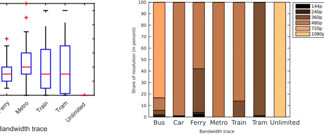
Played Resolution and 6daptation Events In Figure 7 the number of adaptation events, that occurred during one video, is showed. We can see that the median number of adaptation events is less or equal four. In the scenario ‘Metro’, it was exactly four, in case of the ‘Bus’ the least adaptation events of all scenarios with limited bandwidth happen, the median number is one. Interestingly, in case of unlimited bandwidth, no adaptation events happen. This means, that from the beginning on the highest quality was selected, in contrary to the Shaka player, where in this scenario exactly one adaptation event occurs.
Bus Car
Ferry Met ro
Train Tram Unlimit
ed
Bandwidth trace 0
2 4 6 8 10 12
Numberofadaptationevents
Fig. 7. YouTube: number of adaptation events.
Fig. 8. YouTube: played resolution.
Figure 8 shows the share of the resolution that has been played, which ranges from 144p to 1080p. In case of unlimited bandwidth, the highest quality was played all the time. In the ‘Bus’ scenario, 80% of the time the 720p version was played.
In all other scenarios a lower quality was played. The lowest quality was played in the ‘Tram’ scenario, where the player selected the 360p representation layer most of the time.
Stalling In Figure 10, the number of stalling events per video is showed for ev- ery bandwidth scenario, whereas Figure 9 shows their duration. It can be noted, that the median number of stalling events in case of ‘Bus’ and ‘Ferry’ is zero. In the scenarios ‘Train’ and ‘Tram’ it is one. A massive number of stalling events oc- curred in the ‘Metro’ and the ‘Car’ scenario, which also have a large variance in the number of these events.
The length of stalling events is mixed. In all scenarios apart of ‘Train’, the me- dian length is below ten seconds. But the stalling events can also be very long, especially in the scenarios ‘Car, ‘Metro’, and ‘Train’, where there are stalling times up to 150 s.
Bus Car
Ferry Metro Train Tram Unlimited Bandwidth trace
0 50 100 150
Duration of stalling events (in seconds)
Fig. 9. YouTube: stalling duration.
Bus Car
Ferry Metro Train Tram Unlimited Bandwidth trace
0 5 10 15
Number of stalling events
Fig. 10. YouTube: number of stalling events.
. Conclusions Regarding Wasted Traffic
During all experiments, the buffer level was monitored. In order to assess the
potentially wasted bandwidth, we evaluated the buffer status during the playback
of the video. This is done for the YouTube player and the Shaka player. The Shaka player is evaluated with four different buffer configurations. In the following we focus on two configurations one with the buffer size of 90 s and one with 180 s, each with a ten second rebuffering goal. During the playback of the video, each second the current buffer level is written to a log file. Only the readings while the video is playing are selected. Now, for every second of the video the average buffer level is calculated and plotted. This is repeated for every bandwidth scenario.
When the user aborts the playback of the video, the video in the buffer is not needed, hence the bandwidth used for it is wasted. In these diagrams, the average buffer fill level for every scenario can be read directly.
Figure 11 shows this for the Shaka player with a buffer size of 90 s, while in Figure 12 the Shaka player comes with a buffer size of 180 s. In the scenario with the 90 s buffer size, in all scenarios with limited bandwidth, there is a buildup- phase in which the average buffer level rises, a steady phase, in which the buffer level remains at about the same level and a final degradation phase, in which the buffer is emptied, until at the end of the video when the buffer is empty. In the sce- nario with the buffer size of 180 s, which is showed in Figure 12 the steady phase is less distinguished, the average buffer level slowly increases until the degrada- tion phase. In both scenarios, in case of unlimited bandwidth, the buffer is filled completely all the time.
Figure 13 shows the case of the YouTube player. It takes about 200 s until the average buffer level reaches a stable level for all scenarios. The average buffer level never rises above 120 s, during the stable phase it remains between 80 s and 120 s.
Interestingly, in case of unlimited bandwidth, the buffer level remains at about 40 s.
Fig. 11. Shaka player with a buffer size of 90 s: average buffer level over all test
runs during the video, thus the potentially wasted bandwidth.
Fig. 12. Shaka player with a buffer size of 180 s: average buffer level over all test runs during the video, thus the potentially wasted bandwidth.
0 100 200 300 400 500
Time in video in seconds 0
20 40 60 80 100 120 140
Buffer level in seconds Bus
Car Ferry Metro Train Tram Unlimited
Fig. 13. YouTube player: average buffer level over all test runs during the video, thus the potentially wasted bandwidth.
Conclusions
In this paper, we investigated the influence of the buffer size on the playback be- havior of two different HAS players in real commuting scenarios. We compared different buffer configurations of the Shaka player and the standard behavior of the YouTube player.
We could see that a larger buffer, above a certain size, does not increase the
played video quality. That means, the maximum buffer size does not influence
playback so it could theoretically be as high as anyhow possible. However, in terms
of bandwidth consumption, the possible wasted traffic has to be considered. This
study showed, that considering the large share of the overall traffic, that video
streaming accounts for [1], on provider scale, there is a massive saving potential by
limiting the buffer size accordingly. This applies especially in the scenario where
the available bandwidth is much higher than the average video bandwidth. In these cases, the buffer gets filled almost immediately, and as soon as the user aborts the video, all this bandwidth is wasted. As stated before, 20% of all YouTube videos were aborted by users within the first ten seconds. With the Shaka player and a buffer size of 180 s, this means that in those cases at least 18 times more video was transmitted than actually played. In the same scenario, the YouTube player still downloads more than 30 s of video unnecessarily.
One possibility to solve this issue is to leave it to the user to select the buffer size. In [16] it was proposed to allow the user to manually select the players’ be- havior. But as users typically stick to the default settings [3], this will probably only have success in limited cases, like if the user wants to watch a movie without in- terruptions, and knows that the available bandwidth is not sufficient. To do so, knowledge about the bandwidth and planning is required, so that most users will not use this possibility.
This leads to the conclusion that the optimal buffer size is limited. Above a cer- tain buffer size, the overall quality does not further increase. For the sake of eco- nomic bandwidth usage, it should be an option to strictly limit the buffer size in case the available bandwidth is much higher than the video data rate. This can be done by making the buffer size adaptive, like done in [12]. Another option is the YouTube approach, where the buffer size depends on the video quality [17].
In case of high available bandwidth, the player selects the best video quality, and the buffer size is automatically lowered. It can be stated that an implementation is easy, as rate-adaptive video players like the YouTube player or the Shaka player already come with a module for bandwidth estimation.
References
1. Sandvine: Global Internet Phenomena Report: Africa, Mid- dle East, and North America (2015) https://www.sandvine.
com/downloads/general/global-internet-phenomena/2015/
global-internet-phenomena-report-latin-america-and-north-america.
pdf. Last accessed on 14th January 2017.
2. Hossfeld, T, Egger, S. Schatz, R.: Initial Delay vs. Interruptions: Between the Devil and the Deep Blue Sea, 2012 Fourth International Workshop on Quality of Multimedia Experience, Yarra Valley, VIC, pp. 1-6 (2012)
3. Finamore, A., Mellia, M., Munafò, M. M., Torres, R., Rao, S. G.: YouTube Everywhere:
Impact of Device and Infrastructure Synergies on User Experience. In: Proceedings
of the 2011 ACM SIGCOMM Conference on Internet Measurement Conference, pp.
345-360 (2011)
4. Sen, S., Joe-Wong, C., Ha, S., Chiang, M.: Pricing data: A look at past proposals, current plans, and future trends. CoRR, abs/1201.4197 (2012)
5. Balasubramanian, N., Balasubramanian, A., Venkataramani, A. (2009, November). En- ergy consumption in mobile phones: a measurement study and implications for net- work applications. In: Proceedings of the 9th ACM SIGCOMM conference on Internet measurement conference, pp. 280-293 (2009)
6. Seufert, M., Egger, S., Slanina, M., Zinner, T., Hobfeld, T., Tran-Gia, P. (2015). A sur- vey on quality of experience of HTTP adaptive streaming. In: IEEE Communications Surveys & Tutorials, 17(1), pp. 469-492 (2015)
7. Mangla, T., Theera-Ampornpunt, N., Ammar, M., Zegura, E., Bagchi, S.: Video through a crystal ball: effect of bandwidth prediction quality on adaptive streaming in mobile environments. In: Proceedings of the 8th International Workshop on Mo- bile Video, p. 1 (2016)
8. Riiser, H., Endestad, T., Vigmostad, P., Griwodz, C., Halvorsen, P.: Video stream- ing using a location-based bandwidth-lookup service for bitrate planning. In: ACM Transactions on Multimedia Computing, Communications, and Applications, 8(3), 24 (2012)
9. Hao, J., Zimmermann, R., Ma, H.: GTube: geo-predictive video streaming over HTTP in mobile environments. In: Proceedings of the 5th ACM Multimedia Systems Con- ference, pp. 259-270 (2012)
10. Li, X., Dong, M., Ma, Z., Fernandes, F. C.: Greentube: power optimization for mobile videostreaming via dynamic cache management. In: Proceedings of the 20th ACM international conference on Multimedia, pp. 279-288 (2012)
11. Tian, G., Liu, Y.: On adaptive HTTP streaming to mobile devices. In: Packet Video Workshop (PV), 2013 20th International, pp. 1-8 (2013)
12. Wu, D., Huang, J., He, J., Chen, M., Zhang, G.: Toward cost-effective mobile video streaming via smart cache with adaptive thresholding. In: IEEE Transactions on Broad- casting, 61(4), pp. 639-650 (2015)
13. Wamser, F., Seufert, M., Casas, P., Irmer, R., Tran-Gia, P., Schatz, R.: YoMoApp: A tool for analyzing QoE of YouTube HTTP adaptive streaming in mobile networks. In:
2015 European Conference on Networks and Communications (EuCNC), pp. 239-243 (2015)
14. Casas, P., Seufert, M., Schatz, R.: YOUQMON: A system for on-line monitoring of YouTube QoE in operational 3G networks. In: ACM SIGMETRICS Performance Eval- uation Review, 41(2), pp. 44-46 (2013)
15. Riiser, H., Vigmostad, P., Griwodz, C., Halvorsen, P.: Commute path bandwidth traces from 3G networks: analysis and applications. In: Proceedings of the 4th ACM Multimedia Systems Conference, pp. 114-118 (2013)
16. Hoßfeld, T., Moldovan, C., Schwartz, C.: To each according to his needs: Dimension-
ing video buffer for specific user profiles and behavior. In: 2015 IFIP/IEEE Interna-
tional Symposium on Integrated Network Management (IM), pp. 1249-1254 (2015)
17. Sieber, C., Blenk, A., Hinteregger, M., Kellerer, W.: The cost of aggressive HTTP
adaptive streaming: Quantifying YouTube’s redundant traffic. In: 2015 IFIP/IEEE
International Symposium on Integrated Network Management (IM), pp. 1261-1267
(2015)
On the Probability of Meeting Deadlines in IP-based Real-time Communication
Alexander Beifuß University of Hamburg,
Vogt-Kölln-Straße 30, 22527 Hamburg, Germany
Abstract. Today we observe many different real-time services on the In- ternet, though, this network cannot provide any guarantees regarding the quality of data transmissions. For this reason, various distinct ap- proaches (e.g., codecs, buffers, algorithms, and protocols) have been developed with the goal to improve the transmission of real-time data.
Even if each solution is unique on its own, all of them aim for the same objective: to make sure that the data arrives at the receiver in time.
In this paper, we investigate this aspect and present a straightforward and uniform approach to estimate the end-to-end delay of packet trains based on the convolution of the probability distributions of an initial delay and of the inter-arrival times at the receiver. We provide a de- tailed mathematical formulation of our model and share considerations regarding the applicability of our model. We implemented a proof-of- concept and conducted an empirical study with real measurements to evaluate our model.
Key words: real-time services, inter-arrival times, end-to-end delay, packet trains, probability distributions, convolution
Introduction
Today many different real-time services use the Internet: video streaming, video
conferencing, and voice over IP (VoIP) are well-known examples, but the spectrum
is indeed much broader (e.g., in the fields of mobile computing [24], gaming [8],
telemedicine [10], sensor networks [11][2], and robotics [4][25]).
According to Cisco, alone “the sum of all forms of IP video, which includes Internet video, IP VoD, video files exchanged through file sharing, video-streamed gaming, and video conferencing, will continue to be in the range of 80 to 90 percent of total IP traffic” [7] until 2020. This underlines the considerable importance of the subject of this work.
By definition, real-time services have to respect delay bounds, otherwise they are not able to provide the required quality to the end user [12]. Although, there are techniques to provide priority to real-time flows (e.g. IntServ, DiffServ, or MPLS), the Internet cannot generally provide guarantees when data is transmitted be- cause of its store-and-forward architecture and its limited resources which are shared among the users. Hence, the Internet generally offers a best effort trans- mission service only. Many different techniques have been developed that address this issue and the challenging task to improve the transmission of real-time data.
For example, information dispersal schemes aggregate resources of multiple net- works [29], adaptive encoding [28] adjusts the amount of data according to the available resources, playout buffers [16] relax the deadline constraints, and priori- tization strategies [3] favor real-time traffic over other best effort traffic.
Even if these techniques are very diverse, all of them aim for the same objective:
to increase the probability that the real-time data arrives timely at the receiver.
Therefore, gaining knowledge about the probability at which network packets will arrive in time is the key to assess and improve existing approaches and to inspire for novel solutions.
Many researchers have considered this topic. Rubin [23] presented a queuing
theory model to determine the distribution of message delays over a multi-channel
communication path. His model considers messages with arbitrary distributed
message lengths and divided into fixed length packets arriving according to a
Poisson process. Wolfinger [27] modeled the end-to-end delay of file transfers by
means of analytical tandem queuing networks, where the total end-to-end delay
for a file transfer was decomposed into the average delay of the first message and
the sum of average inter-arrival times of the messages at the receiver. Evequoz
and Tropper [9] developed a heuristic to compute the mean end-to-end delay of
multi-packet messages in lightly loaded packet switching networks with flow con-
trol. Papagiannaki et al. [21] found that the tail of the single-hop queuing delay
through a router fits a Weibull distribution. Hernández and Phillips [15] proposed
a Weibull Mixture Model to characterize the end-to-end Internet delay for single packets. Burchard and Liebeherr [6] as well as Fidler [13] use network calculus to derive probabilistic delay bounds for tandem servers. Bisnik and Abouzeid [5]
modeled the random access MAC of IEEE 802.11 and derived a closed expression for the end-to-end delay in multi-hop wireless networks.
In this paper, we investigate the end-to-end delay of packet trains from a black- box perspective and present a unified empirical model to estimate the probability distribution of end-to-end delays of packet trains. In addition to the mathematical formulation of our model we evaluate the quality of our model in an empirical case-study with real-world measurements.
The remaining part of this paper is structured as follows. First, we present our communication model and derive our model for estimating end-to-end delays of packet trains in Section 2, which is evaluated in Section 3. Considerations regard- ing the on-line applicability of our model are shared in Section 4. Finally, we con- clude our work and provide an outlook for future work in Section 5.
Approach
In this section we present a rather general communication model of real-time systems and provide our assumptions and some basic definitions. Based on that, we derive a probabilistic model of the end-to-end delay of packet trains.
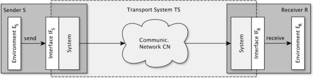
Communication System Model We consider basic sender-receiver systems with a setup as illustrated in Fig. 1. Such systems typically consist of a sender S, a receiver R, and a communication network CN .
First, we specify two target interfaces: IF
Sat the sender and IF
Rat the receiver to decompose the system into three components: the sender environment E
S, the receiver environment E
R, and the transport system T S which consists of CN and the communication system parts within S and R. In this work, T S is considered to be a black box.
E
Sgenerates send events s
iaccording to a certain process. The first bit of the
packets that correspond to s
iwill arrive at IF
Sat the time t(s
i). T S transmits the
data from S to R, and IF
Rwill deliver the data to E
R, so that a receive event r
iis
observed (in consequence of s
i) when the last bit is received at the time t(r
i). Let
us note t(r
i) > t(s
i).
Fig. 1: Illustration of the communication system model
By definition, a real-time service demands a delay bound δ and transmissions with a delay > δ are worthless. Thus, for real-time systems it is of general impor- tance to estimate whether a packet will arrive in time or not.
End-to-end Delay We define end-to-end delay ∆(s
i, r
i) as the length of the time interval between a send event s
iand the consequent receive event r
iobserved at IF
Sand IF
R, respectively (cf. Fig. 2a).
∆(s
i, r
i) := t(r
i) − t(s
i), t(r
i) > t(s
i) (1) Inter-arrival Time We define inter-arrival time (IAT) τ (e
i−1, e
i) as the length of the time interval between two consecutive events e
i−1and e
iof the same arrival process, observed at the interface IF (cf. Fig. 2b). In addition to the expression τ (e
i−1, e
i) we also use the term “IAT at position i” and the identifier τ (i) if the interface is clear. Otherwise, τ
S(. . .) and τ
R(. . .) denote the inter-arrival times at the sender S and the receiver R, respectively.
τ (i) := τ (e
i−1, e
i) := t(e
i) − t(e
i−1), t(e
i) ≥ t(e
i−1) (2)
IF
SIF
Rt t(s
i)
t(r
i)
∆(s
i, r
i) (a)
IF
τ (e
i−1, e
i) t t(e
i−1) t(e
i)
(b)
Fig. 2: Visualization of (a) end-to-end delay, and (b) inter-arrival time
Packet Trains Without loss of generality, we consider the sender process to produce so-called trains of n ≥ 1, n ∈ N
+send requests at once, where N
+denotes the set of natural numbers without 0 ( N
+:= {1, 2, 3, . . .} ). We assume that all packets of the train are delivered to IF
Sback-to-back at the same instant, such that
t(s
j) = t(s
k), ∀j, k with 1 ≤ j ≤ k ≤ n (3) A real-world example for a packet train generating process is live video streaming.
A camera captures pictures at a specific frame rate (e.g., 24 Hz). The picture data is likely to exceed the maximum allowed length of IP packets, thus, single pictures are typically segmented and carried by n > 1 IP packets.
In this work, we focus on packet trains. As of now, {s
i: 1 ≤ i ≤ n} denotes the ith send event of the packet train. Along with that, {r
i: 1 ≤ i ≤ n} denotes the ith delivery event of a packet train. If not stated otherwise, s and r now refer to the send and receive events of packet trains, respectively. Accordingly, a send event of a train of the size of n packets occurs when the first bit of the first packet is sent to IF
S, and a receive event occurs when the last bit of the nth packet train data is delivered by IF
R. Therefore, we define t(s) := t(s
1) and t(r) := t(r
n).
We postulate, that the packets of a packet train that propagates through T S will suffer a constant delay (i.e., the propagation delay), so that, we can conclude
∆(s, r
1) > 0. Moreover, packets of a certain packet train will disperse during trans- mission because of variable delays, e.g., variable queuing delays caused by cross traffic or due to possibly varying data rates, e.g., in the case of dynamic resource al- location (e.g., WiFi RTS/CTS or LTE SC-FDMA). As we suppose that T S does not reorder packets, we can conclude τ
R(r
i, r
i+1) > 0. This assumption is generally not completely fulfilled, but, at least, reordering is rather unlikely in today’s In- ternet and in practice we can simply detect reordering and exclude corresponding packets before applying our model.
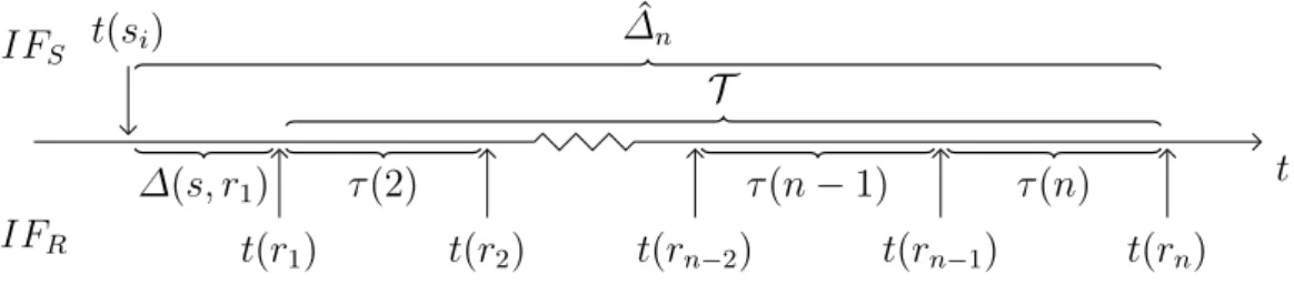
According to (1) we define packet train end-to-end delay as ∆ ˆ
n:= ∆(s, r
n).
Fig. 3 illustrates that ∆ ˆ
ncan be decomposed into the sum of an initial delay (for the transmission of the first packet), followed by a sum of n − 1 IATs (for the delivery process of the remaining packets).
∆ ˆ
n= ∆(s, r
1) +
n
∑
i=2τ (i) (4)
IF
SIF
R∆(s, r
1) t
T
∆ ˆ
nτ (2) t(s
i)
t(r
1) t(r
2)
τ(n − 1) τ (n)
t(r
n−2) t(r
n−1) t(r
n)
Fig. 3: Visual explanation of inter-arrival time
Generally, the probability distribution of the sum Z = X + Y of independent continuous random variables with densities f (x) and g(y) equals the convolution of the individual probability distributions of the random variables [17].
h(z) = (f + g)(z) = ∫
∞
−∞
f (x)g(z − x)dx (5)
We assume the ith term of ∆ ˆ
nto be an independent random variable X
ithat follows a particular probability distribution D
i. If all the individual D
iare known, then, we can calculate the probability distributions of the end-to-end delay D ˆ
nof
∆ ˆ
nby means of convolution:
D ˆ
n∼
n