Building A Hedgehog Pin Array Haptic Interface

Building A Hedgehog Pin Array Haptic Interface

Aline Abler

Master Thesis February 2021

Supervisors:

Dr. Juan Zarate Thomas Langerak

Velko Vechev

Prof. Dr. Otmar Hilliges

Abstract

We present Hedgehog, a self-contained spherical pin array haptic device that can function as a handheld controller and produce cutaneous haptic sensations to the user’s palms. Our design uses 86 passive magnetic pins and a single central omni-directional electromagnetic driver, allowing it to render targeted, directional haptic feedback to the user.

We describe the design choices and hardware implementation of our prototype, evaluate its characteristics, and test its haptic performance in a JND (just noticeable difference) user study.

Finally, we demonstrate its applicability in a number of sample applications, including a racing car game and a direction indicator. The applications showcase how our device can help improve video game immersion, or how it could be utilized as an aid for the visually impaired.

Our work shows how using a single central driver greatly reduces the complexity of manufac- turing and control of our device when compared to one with individually actuated pins, while still providing a rich haptic experience.

To aid in the design of passive magnetic arrays and facilitate the selection of hardware parame- ters, we further present a novel method of approximating vertical forces on individual magnets within a spherical array and predict its behavior, i.e., whether the magnets have a stable resting position and how they react to externally applied electromagnetic forces. Our method gener- alizes to other shapes of magnet arrays in which the magnets are constrained to move only vertically.

i

Contents

List of Figures v

List of Tables vii

1 Introduction 1

1.1 Contributions . . . . 2

1.2 Related Work . . . . 2

1.2.1 Pin Array Displays . . . . 3

1.2.2 Single-actuator systems . . . . 3

2 Design 5 2.1 Pin design . . . . 5

2.2 Magnetic force approximation . . . . 6

2.2.1 Method validation . . . . 11

2.3 Choice of parameters . . . . 13

2.4 Device construction . . . . 16

3 Evaluation 19 3.1 Hardware evaluation . . . . 19

3.1.1 Pin force . . . . 19

3.1.2 Pin extension . . . . 21

3.1.3 Activation spread . . . . 22

3.1.4 Comparison to Approximation Results . . . . 22

3.2 User Study . . . . 23

3.2.1 Experiment 1: Force Absolute Threshold . . . . 24

3.2.2 Experiment 2: JND of Force . . . . 24

3.2.3 Experiment 3: JND of Speed . . . . 25

3.2.4 Discussion . . . . 26

4 Application 29 4.1 Racing game . . . . 29

4.2 Orientation indicator . . . . 30

5 Limitations and Future Work 31

6 Conclusion 33

Bibliography 35

iii

Contents

List of Figures

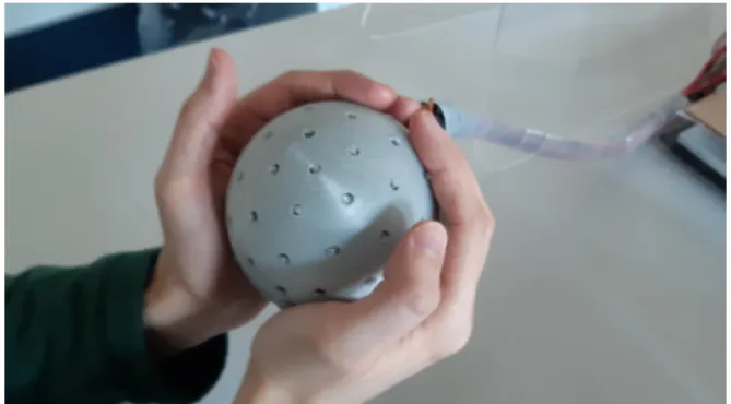
1.1 The Hedgehog Pin Array Haptic Interface . . . . 1

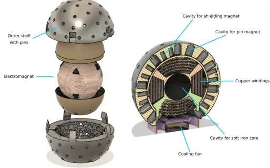
2.1 Exploded view and cross-section of the prototype design . . . . 6

2.2 Diagram of haptic pin construction . . . . 7

2.3 Example of magnet arrangement in an array . . . . 7

2.4 Candidate Goldberg polyhedra . . . . 7

2.5 Illustration of function parameters . . . . 9

2.6 Example of magnetic force function . . . . 10

2.7 Setup of the force validation measurement . . . . 11

2.8 Comparison between measured and approximated (calculated) forces. . . . 12

2.9 Simulation results of force induced by our electromagnet on differently sized rod magnets . . . . 13

2.10 Comparison between characterizations of different array configurations . . . . 15

2.11 The finished prototype . . . . 17

3.1 Measurement of force exerted by a pin on the user’s skin . . . . 20

3.2 Measurement of pin extension distance . . . . 21

3.3 Comparison of force simulation to force and offset measurements . . . . 23

3.4 Example of the staircase procedure . . . . 25

3.5 JND study . . . . 27

4.1 A user enjoying the racing game demo . . . . 29

v

List of Figures

List of Tables

2.1 Polyhedron faces and theoretical pin extension . . . . 14 2.2 Parameters chosen for our prototype . . . . 16 3.1 Fitting results of pin force measurement . . . . 20

vii

List of Tables

1

Introduction

Handheld input devices are prevalent in human-computer interaction and range from computer mice to mobile phones and game or VR controllers. While primarily used as input devices, such controllers (particularly mobile phones and game controllers) are often capable of render- ing vibrotactile feedback, providing a haptic sensation to the user. Haptic feedback has many uses such as improved game immersion or notifying the user of certain events. However, the vibrotactile actuators are limited in their ability to convey more precise sensations of shape, force, or direction.

Pin array haptic interfaces, being able to render more precise haptic feedback, have been an ac- tive area of research for years. They come in the form of stationary devices [Leithinger et al. 2014], portable devices [Zarate et al. 2017], wearables [Vechev et al. 2019] and handhelds [Chen et al. 2019].

Typically, each pin can be actuated individually, which makes not only the device’s hardware complexity grow considerably when more pins are added, but also the complexity of any soft- ware controlling the device.

In this thesis, we explore the use of a magnetic pin array for haptic feedback rendering in controllers. We leverage a single omni-directional electromagnet to actuate a spherical array of

Figure 1.1: The Hedgehog Pin Array Haptic Interface.

1 Introduction

passive magnetic pins, significantly simplifying the manufacturing and operation of our device compared to traditional pin array interfaces. The spherical form factor enables new interaction paradigms, for example in combination with IMU (Inertial Measurement Unit) sensors to infer orientation.

Our work directly builds upon the Omni haptic prototype [Langerak et al. 2020], which uses an omni-directional electromagnet to induce force feedback on a passive magnetic tool held by the user. We are able to re-use hardware components of Omni, such as the electromagnet, cooling system, and the hardware control interface. We newly design a passive magnetic pin array to be mounted on top of the electromagnet, as well as new control software for the altered device.

Designing a pin array based on passive magnets requires considerations such as the magnets’

sizes, their placement, and the capabilities of the driving electromagnet. These parameters have an influence on the resulting device’s size and weight, maximum force output, and pin array density. Finding an optimal choice in that parameter space requires efficient exploration of the available options. We introduce a novel technique for estimating passive magnetic forces in pin arrays, allowing us to predict the stability and behavior of given arrays and select the optimal parameters for our prototype.

We assess the capabilities of our approach through a JND (just noticeable difference) user study exploring the operational range and limitations of our prototype device. Additionally, we present two sample applications to showcase potential use-cases for such a spherical pin array interface.

1.1 Contributions

• A novel method of evaluating the mutual interaction in non-planar arrays of passive mag- nets, allowing prediction of the array’s behavior and facilitating the selection of optimal array parameters (i.e. magnet sizes and placement)

• A handheld controller that renders haptic feedback to the user’s palm through passive magnetic pins, based on hardware components re-used from the Omni haptic proto- type [Langerak et al. 2020]

• A user study measuring the user’s force and speed sensitivity with respect to our device, through which we determine the operational range of our prototype and the minimum change in intensity that can be sensed by the user

• Sample applications demonstrating the capabilities of the prototype e.g. in video game settings, or as an aid for the visually impaired

1.2 Related Work

Nowadays, the most commonly used mechanism for haptic feedback are vibrotactile actuators.

With their small form factor and low manufacturing cost, they are easily embedded in game con-

trollers, mobile phones, and more recently in VR controllers. However, vibrotactile haptic feed-

1.2 Related Work

back is often coarse and imprecise, and while this limitation can be overcome, e.g., through the use of several vibrotactile motors and interpolating between them [Israr and Poupyrev 2011], in its most common use vibrotactile feedback is one-dimensional and fails to convey shape or directional information.

Many alternatives to vibrotactile feedback have been explored and often succeed in convey- ing higher fidelity haptic sensations—both cutaneous and kinesthetic, e.g. [Massie et al. 1994]

[Yamaoka and Kakehi 2013] [Stamper 1997] [Van der Linde et al. 2002]. These devices are usually anchored rigidly, allowing them to supply larger forces with great precision. While these prototypes are appropriate for high-end applications such as tele-operation, their size and lack of portability makes them unsuitable for handheld use.

Handheld and wearable haptic devices can provide high fidelity haptic feedback, e.g. through the use of electrostatic brakes [Hinchet et al. 2018] or tilt platforms [Benko et al. 2016]. These devices are often hard to manufacture, and additionally, controlling all the degrees of freedom they provide incurs complexity on the control software. Our approach seeks to simplify these aspects, particularly the latter, by controlling multiple movable components with a single actu- ator.

1.2.1 Pin Array Displays

Pin array displays have been around for a while and come in a large variety of execution. Most commonly, such devices are stationary and can thus make use of large activation mechanisms, e.g. linear actuators [Leithinger et al. 2014]. Other devices make use of electromagnetic ac- tuation [Zarate et al. 2017] [Yang et al. 2009] which allows for a smaller, portable form factor.

TacTiles [Vechev et al. 2019] is a wearable device that uses individually controlled pins in spe- cific locations on the palm to render haptic feedback. Haptivec [Chen et al. 2019] is a pin array display for handheld use, making it most similar to our work. Haptivec’s pins are individually actuated using solenoids.

1.2.2 Single-actuator systems

Unlike previous pin array designs, our system uses a single actuator to drive its pins. Haptic interfaces using a single actuator typically have a single point of contact for the user, such as the Foldaway prototype [Mintchev et al. 2019], where users can interact with a small 3-DOF platform mounted to a controller. Our design, being a pin array, naturally has multiple contact points on its entire surface.

The use of 3-DOF omni-directional electromagnets for haptic feedback rendering has been ex- plored in Omni [Langerak et al. 2020], where said electromagnet is used to render force feed- back to a passive magnetic pen held by the user. Omni serves as the primary inspiration for our work, and several hardware components of the Omni prototype were re-used, most notably the electromagnet itself.

3

1 Introduction

2

Design

Our haptic interface leverages a single central omni-directional electromagnet to actuate its pins, which are attached to passive magnets (Figure 2.1). This imposes the restriction that all these passive magnets have to be oriented in the same direction (inward or outward), such that the single electromagnetic driver can actuate them all equally. To avoid magnetic cross-talk due to the passive magnets repelling each other, an arrangement has to be found in which all passive magnets have a stable resting position that is not affected by neighboring magnets moving around.

2.1 Pin design

The haptic pins are small acrylic cylinders attached to passive magnets (pin magnets), which are embedded in a plastic casing that only allows the pin magnets to move vertically (see Fig- ure 2.2).

In order to avoid magnetic cross-talk between pin magnets and to keep the entire array in a stable configuration, smaller shielding magnets of opposite polarity are inserted in between pin magnets (also depicted in Figure 2.2). These will hold the pin magnets in a stable resting position when the electromagnet is deactivated. We choose a hexagonal arrangement for pin and shielding magnets.

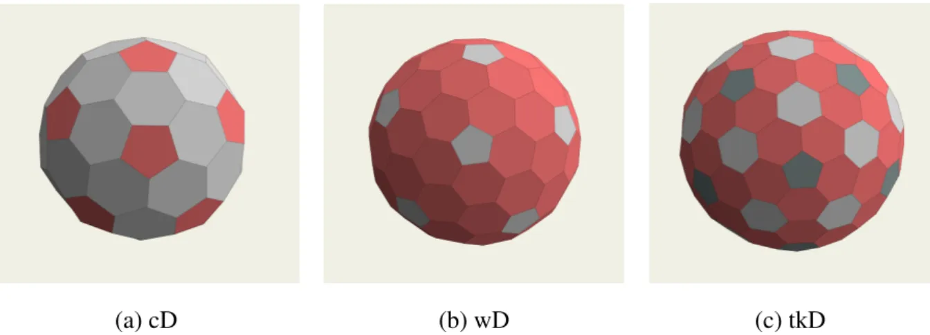
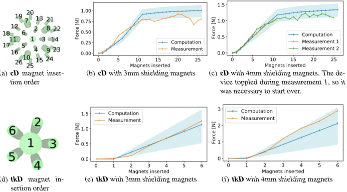
Since plain hexagonal arrangements are planar and cannot be directly wrapped around a sphere, we pick the magnet locations based on an icosahedral Goldberg polyhedron (see Figure 2.4).

The icosahedral Goldberg polyhedra form an infinite class of convex polyhedra consisting of

hexagons and pentagons, which allows for a hexagonal magnet arrangement with relatively few

irregularities. Figure 2.3 shows an example of such a Goldberg arrangement of pin and shielding

magnets. Throughout this thesis, specific Goldberg polyhedron based arrangements are referred

to by the corresponding Conway polyhedron notation [Conway et al. 2016].

2 Design

Figure 2.1: Exploded view and cross-section of the prototype design. The larger cavities in the outer- most shell hold the pin magnets, allowing for a few millimeters of vertical movement and containing a smaller hole for the pins to extend through. The smaller cavities hold the shield- ing magnets, which remain stationary. Magnets are inserted from the inside and held in place with a thin hemispherical shell, which in turn encases the electromagnet.

Choosing the sizes (and, as a result, strengths) of pin and shielding magnets presents an opti- mization problem. The following aspects need consideration:

• The electromagnet can induce larger forces in stronger magnets, but at the same time, small magnets are desirable as they allow for a more compact design and a denser pin array.

• The shielding magnets have to be strong enough to retain the pin magnets in their resting positions, but that retaining force has to be small enough to be overcome by the electro- magnet, whose maximum force output is constrained by overheating concerns. In other words, the relative sizes of pin and shielding magnets have to be chosen such that the latter are only just able to retain the former, but not more.

2.2 Magnetic force approximation

In order to determine whether a given magnet arrangement has a stable resting position, it is necessary to calculate the vertical force induced on a specific pin magnet by all other magnets.

Only the vertical force is of interest, as the magnet’s lateral movement is constrained and ro-

tation is irrelevant thanks to our use of cylindrical magnets. To calculate this vertical force,

we developed a method of approximating passive magnetic forces in a pin array consisting of

differently sized and oriented magnets.

2.2 Magnetic force approximation

Figure 2.2: Diagram of haptic pin construction.

Figure 2.3: Example of magnet arrangement in an array.

Shielding magnets are rendered in red, pin magnets in green.

(a) cD (b) wD (c) tkD

Figure 2.4: Candidate Goldberg polyhedra. To achieve a spherical hexagonal arrangement, a pin magnet is placed at the center of each face and a shielding magnet is placed at each vertex. The Conway polyhedron notation [Conway et al. 2016] of each polyhedron is given.

The colors indicate groups of faces which are equal w.r.t. symmetry.

While there exist Goldberg polyhedra with arbitrarily many faces, at some point the magnet’s size makes it impossible to place that many on a fixed-size sphere. In our case, (c) is the densest possible arrangement.

7

2 Design

Our method relies on three observations:

• Our setting includes only permanent magnets as well as the electromagnet’s core, which magnetizes linearly. No non-linear magnetic components are included, which allows us to sum up partial magnetic forces to obtain an overall result. Using this technique, it thus suffices to calculate the vertical magnetic force only between each pair of permanent magnets.

• For any given magnet in an arrangement, most of the other magnets are sufficiently far away such that the magnetic force between them can be accurately estimated by modeling both magnets as magnetic dipoles [Yung et al. 1970]. The dipole model provides a closed- form solution and can be easily calculated.

• For the few remaining magnet pairs that are too close together for use of the dipole model, it is feasible to utilize FEA (Finite Element Analysis) simulations, which can accurately solve the Maxwell equations for meshed geometries. The results, while sufficiently accu- rate, are computationally costly, so we rely on them only for these few remaining magnets.

Our FEA results are obtained using Comsol Multiphysics with its magnetic modules, which are utilizing Maxwell differential equations in a meshed volume. In our case, this volume contains a pair of passive magnets and the surrounding air.

This method allows us to calculate the vertical force induced on a specific magnet by all other magnets in the arrangement, using only a small number of computationally expensive FEA simulations.

We can further improve upon the method by re-using FEA results. To this end, we leverage the fact that our magnet positions are constrained to the surface of a sphere. The relative po- sition between any pair of magnets is thus given by the angle between their position vectors (Figure 2.5).

We consider the function P airF orce

(α) that calculates the vertical force acting between two passive magnets m

and m

given their relative angle α. For large α, we utilize the dipole model to directly calculate an approximate result. To obtain results for small α, we first use a selection of angles α for which we simulate the result of P airF orce

(α) using FEA; with these results we can create a piece-wise linear interpolation of the function P airF orce

(α), from which we can sample an approximate result for any α. A plot of the thus approximated function P airF orce

(α) is given in Figure 2.6.

P airF orce

(α) =

( F EA

(α) α < 30

DipoleM odel

(α) otherwise. (2.1) Having obtained an approximation of P airF orce

(α), we are now able to re-use it for vertical force calculations on different magnet arrangements, provided they are all constrained to the same sphere.

To accommodate for the use of differently sized magnets, the function P airF orce

(α) is

parameterized by the sizes of the two magnets in question. The two magnet sizes m

and m

are given by the magnets’ heights and diameters. For each combination of magnet sizes in an

2.2 Magnetic force approximation

Figure 2.5: Illustration of parameters for function P airF orce

(α, o). The function’s result is the vertical force induced on m

by m

. Both magnets have the same polarity (north pointing outwards).

arrangement, F

(α) is approximated anew using the method detailed above.

Although the function P airF orce

(α) has to be calculated anew when changing magnet sizes, the same is not necessary when the polarity of either magnet changes. A change in polarity simply represents a sign change of the function result, which can be taken into account when summing up individual results.

We can now calculate an approximation of the vertical force F

induced on magnet m by all other magnets in arrangement M:

F

= X

mi∈M\m

P airF orce

(angle(m, m

)) ∗ polarity(m, m

) (2.2)

with

polarity(m

, m

) =

( 1 if m

and m

have same polarity

−1 otherwise. (2.3)

Using our method, we can approximate the vertical force induced on any given pin magnet by all other magnets in an array.

However, in this situation, all magnets remain stationary. Since our pin magnets are able to move outwards, it is necessary to understand how the induced vertical force changes as a magnet moves vertically. In the extreme case, when considering a flat array, the vertical forces would be zero in the resting position, but if a magnet is moved vertically even slightly, these forces could increase dramatically.

To understand the influence of vertical movement on the force, we extend our function by an additional parameter o representing the vertical offset of the first magnet. Figure 2.5 gives an illustration of the function’s parameters. P airF orce

(α, o) is approximated using the same method as before, though the number of required FEA simulations increases with the parameter

9

2 Design

0 20 40 60 80

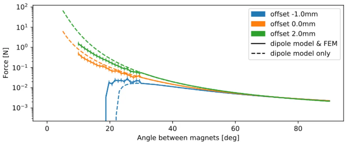
Angle between magnets [deg]

10

10

10

10

10

10

Force [N]

offset -1.0mm offset 0.0mm offset 2.0mm dipole model & FEM dipole model only

Figure 2.6: Example of magnetic force function approximation P airF orce

(α, o) display- ing the vertical force which a magnet with 2mm radius exerts on a magnet with 4mm radius at different angles apart, at various offsets o. Both magnets have a height of 10mm.

In our approximation, values below 30 degrees are found using FEA simulations, values above 30 degrees are found using the dipole model for calculating forces between magnets.

For comparison, the dipole model results for all values are given in this graph in addition to the FEA results.

Vertical markers indicate the points at which a FEA simulation was performed to obtain the result. Values in between are linearly interpolated.

space. In order to evaluate the behavior of a given pin magnet m

, we consider the function F

(o) which calculates the vertical force induced on magnet m

by each other magnet in a given arrangement M for each vertical offset o.

F

(o) = X

mi∈M\mp

P airF orce

(angle(m

, m

), o) ∗ polarity(m

, m

) (2.4)

As we use Goldberg tilings for our magnet arrangements, this vertical force curve F

(o) will not be the same for each pin magnet m

inside a specific arrangement: For example, some pin magnets are surrounded by only five shielding magnets instead of six, so it is to be expected that those display a different force curve than others. To fully characterize the stability of a given array, it is thus necessary to calculate F

(o) for each individual pin magnet on it. This characterization can then be compared between different arrays in order to choose the optimal arrangement for a given sphere size. The characterizations of all our candidate arrangements are displayed in Figure 2.10.

When choosing the optimal arrangement, it is necessary to consider the maximum force the

electromagnet is able to induce in the chosen pin magnets, since that will determine the maxi-

mum distance by which the pins can move. In section 2.3, we go into more detail on how the

optimum was chosen.

2.2 Magnetic force approximation

Figure 2.7: Setup of the force validation measurement.

2.2.1 Method validation

We validate the results of our approximation method by performing a measurement to compare measured vertical forces to our approximation results.

To obtain the measurements, a 3D-printed rig to hold the magnets is mounted on top of a force sensor (FSAGPNXX1.5LCAC5, Honeywell) as depicted in Figure 2.7. Through a hole in the rig, the central magnet can apply force directly to the sensor via the use of a small rod. Magnets are inserted one-by-one into the rig while the sensor force is being measured. All magnets are inserted with the same polarity, resulting in an outwards (downwards) vertical force induced in the central magnet. After each inserted magnet, the currently measured force is sampled.

These sampled values are compared to simulation results of an equivalent arrangement using our method.

The precise force acting on the central magnet is very sensitive to small changes in the mag- net’s vertical offset. Due to the nature of our experiment setup, the exact vertical offset during the experiment can vary by approximately ±0.25mm. To account for this, our comparison in- cludes the forces at offsets +0.25mm and -0.25mm as upper and lower bounds for the expected measurement values.

The experiment was performed in four different configurations; the results are displayed in Figure 2.8. Our approximation holds up fairly well compared to the measurements without any need for curve fitting.

11

2 Design

(a) cD magnet inser- tion order

0 5 10 15 20 25

Magnets inserted 0.00

0.25 0.50 0.75 1.00

Force [N] Computation

Measurement (b) cD with 3mm shielding magnets

0 5 10 15 20 25

Magnets inserted 0.0

0.5 1.0 1.5

Force [N] Computation

Measurement 1 Measurement 2

(c) cD with 4mm shielding magnets. The de- vice toppled during measurement 1, so it was necessary to start over.

(d) tkD magnet in- sertion order

0 1 2 3 4 5 6

Magnets inserted 0.0

0.5 1.0 1.5

Force [N]

Computation Measurement

(e) tkD with 3mm shielding magnets

0 1 2 3 4 5 6

Magnets inserted 0

1 2 3

Force [N]

Computation Measurement

(f) tkD with 4mm shielding magnets

Figure 2.8: Comparison between measured and approximated (calculated) vertical forces as more mag-

nets are inserted into the array. The measurement was performed in different array configu-

rations and with different magnet sizes, to test the general applicability of our approximation

method. The light blue range indicates the range of force resulting in the central magnet be-

ing vertically offset by ±0.25mm.

2.3 Choice of parameters

Figure 2.9: Simulation results of force induced by electromagnet on differently sized rod magnets. The electromagnet is operated at I = 15A and the cylindrical passive magnet is placed vertically directly above at a distance of 35mm, which corresponds to the shortest distance it is physi- cally possible to place a magnet to our electromagnet.

2.3 Choice of parameters

Our prototype re-uses the electromagnet from the Omni prototype [Langerak et al. 2020], so the strength as well as the dimensions of that hardware component are given. The radius of the electromagnet is 35mm, and we opt to place our pin magnets as close as possible to the electromagnet in order to maximize the induced force while keeping the device compact. As a result, our passive magnets are constrained to the surface of a sphere with radius 35mm.

To choose a suitable size for our passive pin magnets, we simulate the maximum force our elec- tromagnet can induce on differently sized rod magnets. We use N45 Neodymium rod magnets with a residual flux density of approximately 1.37 Tesla. Figure 2.9 shows the result of the FEA simulation. It is necessary to pick a magnet in which it is possible to induce sufficient strength (i.e. one from the green, yellow and red regions on Figure 2.9), but in addition it is desirable to pick a small magnet. A magnet with a smaller radius will potentially allow for denser array configurations (i.e. more pins to be placed on the sphere), and a magnet with a smaller height will decrease the total radius of the finished device, making it more compact.

Since, according to our simulation, the magnet’s radius has a larger impact on induced strength than the height, we opted for a shorter magnet at the cost of said larger radius. Our final choice for the pin magnets were thus rod magnets with a radius of 4mm and a height of 10mm. The electromagnet can induce up to 0.4N of force in these magnets.

The magnets’ sizes and that of the sphere on which they rest dictate which specific Goldberg polyhedra are suitable to our purpose. The magnets can only be placed as closely together as their physical size allows. In our case, the sphere radius is 35mm as dictated by the electromag- net’s dimensions, and we chose cylindrical pin magnets with a diameter of 8mm. With that, the polyhedron tkD is the densest pin arrangement possibility (see Table 2.1). Only a finite amount of less dense options exist [Wenninger 1999]. Of these, we have ruled out D (dodecahedron) and tI (truncated icosahedron) for being too sparse (i.e. having too few faces) to provide a rich haptic experience in our setting. The remaining options are cD and tkD of the Class 1 Goldberg

13

2 Design

Configuration Number of faces Maximum pin extension

cD 42 0.8mm / 3.5mm

wD 72 0.2mm / 0.6mm

tkD 92 0.1mm / 0.6mm / 0.7mm

Table 2.1: Polyhedron faces and theoretical maximum pin extension for different configurations. Not all pins within a given configuration reach the same maximum extension, due to irregularities in the hexagonal pattern.

polyhedra and wD of the Class 3 Goldberg polyhedra. All three candidate options are pictured in Figure 2.4.

Figure 2.10 shows the characterizations of all candidate configurations, once each for shielding magnets with a diameter of 3mm and 4mm. It can easily be seen that as the arrays get denser, the curves become more extreme, which is natural—in denser arrangements the magnets are placed closer together and can thus induce larger forces in each other. Furthermore, it is immediately visible that shielding magnets of 3mm diameter are not feasible: The force on the pin magnets is positive (i.e. directed outwards) at all offsets, meaning the magnets will always be pushed away and the arrangement does not have a stable resting position.

With a shielding magnet diameter of 4mm, all arrangements become stable and have a stable resting position close to offset 0. This indicates that in all these arrangements the pins will be retracted when the electromagnet is not powered.

It is not necessary to consider larger shielding magnets, as we are trying to find the weakest shielding magnets that still result in a stable configuration.

Knowing that our electromagnet can induce a force of at most 0.4N on the pin magnets (Fig- ure 2.9), we can read from the graphs in Figure 2.10 what the maximum pin extension would be for each of these configurations. The maximum pin extension corresponds to the difference between these graph’s zero-crossings and the points where they cross -0.4N. This will yield multiple results, which are detailed in Table 2.1

What remains is to choose between having a denser pin array, which has more contact points for the user to feel, and having a pin array in which the pins travel outwards further, which can result in a more pronounced sensation. Since the simulation shows that tkD and wD behave similarly for most of the pins (the exception being those pins on tkD which sit at the center of a pentagon, as they have a more extreme force curve), it can be argued that tkD is better suited between the two. Between tkD and cD, we have opted for the tkD configuration for our prototype, favoring the denser option.

Having chosen the arrangement, Table 2.1 informs our decision on how much vertical space the pin magnets need in order to achieve maximum pin extension. We chose to allow for up to 1.5mm of vertical travel, which more than contains the theoretical pin extension range our electromagnet can achieve with the chosen magnets.

An overview of all chosen parameters is given in Table 2.2.

2.3 Choice of parameters

2.5 0.0 2.5 5.0 7.5 10.0 12.5 offset [mm]

2 0 2 4 6

force [N]

(a) cD with 3mm shielding magnets

2.5 0.0 2.5 5.0 7.5 10.0 12.5 offset [mm]

2 0 2 4 6

force [N]

(b) cD with 4mm shielding magnets

cD (sparsest)

2.5 0.0 2.5 5.0 7.5 10.0 12.5 offset [mm]

2 0 2 4 6

force [N]

(c) wD with 3mm shielding magnets

2.5 0.0 2.5 5.0 7.5 10.0 12.5 offset [mm]

2 0 2 4 6

force [N]

(d) wD with 4mm shielding magnets

wD

2.5 0.0 2.5 5.0 7.5 10.0 12.5 offset [mm]

2 0 2 4 6

force [N]

(e) tkD with 3mm shielding magnets

2.5 0.0 2.5 5.0 7.5 10.0 12.5 offset [mm]

2 0 2 4 6

force [N]

(f) tkD with 4mm shielding magnets

tkD (densest)

Figure 2.10: Comparison between characterizations of different array configurations. The graphs show the function F

(o) (force induced on a pin magnet by all other magnets as the pin magnet is vertically offset from the surface of the sphere). A separate line is plotted for each pin magnet; however, due to symmetry, pin magnets fall into only two or three classes within which the force curves are all equal. For reference, Figure 2.4 shows these symmetries for all candidate configurations.

In a stable array, as a pin’s offset increases, the induced force becomes negative (the pin is pulled back into the array towards its resting position). Once the pin is moved out too far, force turns back to positive as it is now repelled by the other pin magnets. In an unstable array, the shielding magnets are too weak to keep the pin magnets in their resting position;

the forces are positive throughout.

15

2 Design

Parameter Value Reasoning

Electromagnet inherited from Omni proto- type [Langerak et al. 2020]

Hardware availability

Pin magnet 10mm height, 8mm diameter

based on FEA simulation in Figure 2.9

Shielding magnet 10mm height, 4mm diameter

based on evaluation in Figure 2.10

Arrangement tkD based on evaluation in Figure 2.10

Vertical space for pin travel

1.5mm based on evaluation in Table 2.1

Table 2.2: Parameters chosen for our prototype.

2.4 Device construction

The pins are held in two hemispherical 3D-printed casings (Figure 2.1) which are put together into a full sphere, enclosing the electromagnet in the center. The casings allow the pin magnets to move vertically by at most 1.5mm, while the shielding magnets are kept stationary. The pins are cut from acrylic and mounted to the surface of the pin magnets using double-sided tape. The pins can protrude out from the surface of the device through holes in the casing (Figure 2.2).

In between the two pin hemispheres, the electromagnet is held on a 3D-printed rig. Regis- tration notches ensure accurate placement. The electromagnet itself is directly taken from the Omni prototype, and its construction is described minutely in [Langerak et al. 2020]. It uses a 30mm diameter soft iron core surrounded by three mutually orthogonal interwoven copper coils (roughly 150 turns per coil).

To control the generated magnetic force, each magnetic coil is connected to an H-bridge (Pololu G2 18v17) which controls the voltage through pulse width modulation. We can directly control the current given Ohm’s law and the resistance of the coils [Langerak et al. 2020].

A temperature sensor is attached to the electromagnet’s copper coils. The control software uses the temperature readings to prevent overheating. The device can be operated indefinitely at a current of 5A, and current spikes of up to 15A are possible.

As a further aid against overheating, a brushless DC fan (CUI Devices, 0.524 m

/min) is placed at the bottom of the device to allow for cooling of the electromagnet.

A hole at the bottom next to the fan mount allows for connector cables to be run through the

casing.

2.4 Device construction

Figure 2.11: The finished prototype.

The chosen Goldberg configuration, tkD, includes 92 movable pin magnets. However, due to the necessity of mounting a fan and connectors on the device’s underside, 6 of those pins are re- moved, resulting in a final array of 86 actuated pins. Thanks to our approximation method from section 2.2, we were able to verify that despite removing 6 pins and their surrounding shield- ing magnets, the final arrangement still has a stable resting position for all pins and behaves similarly to the full 92-pin version.

17

2 Design

3

Evaluation

We evaluate the performance of our device through a hardware evaluation as well as a user study. The hardware evaluation, detailed in the first section, consists of a series of measurements including pin force and pin extension. The user study is detailed in the second section and examines the operational range of our device and how many different sensations users can distinguish.

3.1 Hardware evaluation

It is necessary to understand the hardware characteristics and limitations for our device in order to consider possible applications and potential points of improvement. Our device is controlled by setting the current in the electromagnet’s coils (I

) through PWM (pulse-width modulation).

This metric cannot be directly compared to other pin array devices, so we must understand how current translates to pin force and extension.

3.1.1 Pin force

To determine the force a pin exerts on the user’s skin, we mounted an analog force sensor (FSAGPNXX1.5LCAC5, Honeywell) to the outside of the device such that the pressure plate of the sensor rests directly above the pin in its resting position (see Figure 3.1(a)). The electro- magnet was powered on, pointing directly at the prepared pin, and actuation electric current (I

) was gradually increased from 0A to 10A. The force measurements were recorded and are displayed in Figure 3.1(b).

The force sensor produces rather noisy measurements, so we fit a linear function to the resulting

data to obtain a good approximation. The result of the fitting is detailed in Table 3.1. Since the

3 Evaluation

(a) Experiment setup. The se- lected pin is a first neighbor to one of the pins inside a pen- tagon face; this is the most common pin type of this par- ticular configuration.

0 2000 4000 6000 8000

Current [mA]

0.2 0.3

Force [N] repetition-1

repetition-2 repetition-3

(b) Experiment result. The experiment was repeated three times.

Individual samples are shown in lighter colors; the darker col- ored lines represent a linear function that was fitted to the sam- ples.

Figure 3.1: Measurement of force exerted by a pin on the user’s skin.

Repetition Fitted linear function Standard error of slope Repetition 1 F = 0.20N + 0.0125

∗ I

±1.5 ∗ 10

(1.2%) Repetition 2 F = 0.19N + 0.0126

∗ I

±1.5 ∗ 10

(1.2%) Repetition 3 F = 0.16N + 0.0138

∗ I

±1.5 ∗ 10

(1.1%)

Table 3.1: Fitting results of pin force measurement.

force sensor is gently pressed onto the pin by the experiment setup, the force value at 0A has to be subtracted; this means only the slopes of the fitted functions are relevant. With the median slope (from Repetition 2), we calculate that the resulting force exerted on the user’s skin is approximately 0.06N at a current of 5A (continuous operation) and approximately 0.2N at a current of 15A (maximum spike current).

The maximum pin force of 0.2N compares well to similar pin array devices. BlindPad [Zarate et al. 2017], MagTics [Pece et al. 2017] and TacTiles [Vechev et al. 2019] all rely on a bi-stable magnetic

latching mechanism for their pins and all report a pin holding force of 0.2N. In all three cases, the bi-stable nature of the mechanism implies that no dynamic adjustment of the pin force is possible, unlike in our case. On the other hand, on those bi-stable devices, the pin force of 0.2N can be applied indefinitely, while on our prototype it is only possible to continually supply 0.06N of force (at 5A). To reach 0.2N, we apply a spike current of 15A, which can be held for approximately 30 seconds before the actuator has to shut down to prevent overheating.

The Haptivec handheld pin array [Chen et al. 2019] relies on solenoids for pin actuation, making it more similar to our prototype in that keeping a pin extended requires continuous current.

[Chen et al. 2019] reports a blocking force of 0.32N for their solenoids.

While our device cannot sustain the maximum pin force of 0.2N indefinitely, our user study

(section 3.2) shows that a lower force is sufficient for the users to clearly feel dynamic pat-

terns. Additionally, the ability to use a reduced pin force and adjust it dynamically adds a new

dimension to our haptic feedback, allowing it to more intuitively convey a measure of intensity.

3.1 Hardware evaluation

(a) Example of a photograph used for ob- taining the measurements. The relevant dimensions are highlighted in red: The diameter of the pin serves as the known reference; the distance between the top of the pin and the pin hole serves as our extension measurement.

0.0 2.5 5.0 7.5 10.0 12.5 15.0 Current [A]

0.0 0.2 0.4 0.6

Pin extension [mm]

(b) Experiment result. Between 8 and 9 photographs were taken for each data point. The graph shows the median of each data point. The measurement for 0A was subtracted from all data points such that a deactivated electromagnet corre- sponds to an extension of 0mm. Error bars denote the stan- dard error of the median, which was found using the bootstrap method [Efron 1982].

Figure 3.2: Measurement of pin extension distance.

3.1.2 Pin extension

Pin extension was measured using photographs taken at different electromagnet activation cur- rents, using a known dimension from the photograph as a reference. Multiple photos were taken to improve accuracy. Of all the thus obtained measurements, we present the median value. The results can be seen in Figure 3.2(b).

During the measurement, the device was cycling between the current values 0A, 5A, 10A, 15A, 10A, 5A, and finally 0A again. That way, we obtain photographs in which the pin has just retracted to its current position from a further-out position, as well as photographs in which the pin has just extended outwards from a further-in position. With this, we hope to negate bias due to hysteresis.

The results correspond well to our simulation results from section 2.2, as discussed further below in subsection 3.1.4.

The maximum pin extension (or stroke length) reported in other similar pin-array devices ranges from 0.8mm in BlindPad [Zarate et al. 2017] to 3.5mm in Haptivec [Chen et al. 2019]. Our device’s pin extension is lower with a maximum of 0.5mm, which makes it hard to sense which pins are actuated in a static setting; however, for dynamic patterns, users can still easily feel the change in pin force and extension, as demonstrated in section 3.2.

21

3 Evaluation

3.1.3 Activation spread

As we use a single central electromagnet to operate all pins, it is not possible to actuate a single pin in isolation. When the magnetic field is pointed at a specific pin, naturally that pin will actuate; however, neighboring pins will react to the magnetic field as well and actuate too, albeit less strongly. As a result, the direction of actuation can not be sensed very clearly, as there is always an entire area of activated pins. On the other hand, activation spread increases the likelihood of a given activation being felt even when the user’s hand does not cover the specific pin being targeted. Activation spread is a result of our choice of actuating mechanism and has to be kept in mind when designing haptic patterns for our device.

Activation spread increases with the activation force, so a larger electromagnetic force not only results in a stronger pin force and larger pin extension, but also in a larger area of activated pins.

3.1.4 Comparison to Approximation Results

The force and pin extension measurements from this evaluation are correlated; applying a given force to a pin will result in a specific extension. This relation is already explored in the magnetic force approximations from section 2.2, so it is reasonable to compare our measurement results to these approximations for verification.

It is important to note that in our measurement, the reference point for pin extension (i.e. the point where extension equals 0) is, naturally, the pin’s resting position when the electromagnet is powered off. However, in the approximations in section 2.2, the reference point for offset is the point where the magnet is exactly 35 mm away from the sphere center, this being the sphere’s radius. In the approximations, offset is given relative to the sphere surface and does not necessarily correspond to the magnet’s resting position.

To account for this, it is sufficient to find the zero-crossing of the graph in Figure 2.10(f), as the point where the force is zero would naturally correspond to the magnet’s resting position.

This zero crossing, for the specific pin on which we performed the measurements, is at 0.45mm.

By adding these 0.45mm to our pin extension measurements, we obtain comparable data. Fig- ure 3.3 shows the result of our comparison.

This comparison shows that our measurements agree with the predictions from section 2.2, lending confidence to the accuracy of our results.

The relation between magnetic force and pin extension depends on the precise arrangement of

pin and shielding magnets, and should one wish to change this relation, a completely new pin

array would need to be constructed. However, predicting this relation ahead of time is easily

possible using our approximation method detailed in section 2.2.

3.2 User Study

0.4 0.5 0.6 0.7 0.8 0.9 1.0

offset [mm]

0.25 0.20 0.15 0.10 0.05 0.00 0.05

force [N]

Simulation result Measurements

Figure 3.3: Comparison of force simulation to force and offset measurements. The graph shows a close- up of Figure 2.10(f) with the results of the measurements on the actual device included in red color. The measurements correspond well to the approximated results, but it is to note that the simulation only includes force samples at offsets 0.5mm and 1mm which have been linearly interpolated.

3.2 User Study

To design interaction patterns for our device, it is necessary to know its operational range.

The goal of this study is to determine the minimum amount of force required for the user to perceive the sensation, as well as the user’s sensitivity to changes in activation force and speed (expressed as the just noticeable difference, or JND). In particular, we aspire to answer the following research questions:

• What is the minimum amount of pin force a user can perceive in a dynamic haptic pattern on our prototype?

• What is the just noticeable difference (JND) of pin force for dynamic haptic patterns on our prototype?

• What is the just noticeable difference (JND) of pattern speed for dynamic haptic patterns on our prototype?

For the two JND experiments (Experiment 2 and 3), reference levels for force and speed had to be chosen. We chose 5A (≈0.06N) as our reference force level, as this is the highest level allowing for continuous activation of the device without overheating, and as such is of special interest. The reference level for speed is 10 pins per second (≈20cm/s); this level was chosen for feeling like a moderate speed to our own subjective perception.

For all experiments, users were asked to place their dominant hand on top of the device, which would play a dynamic circular pattern. Participants were required to wear noise-canceling head- phones during the experiments, to avoid bias due to sounds emitted by the prototype device during operation.

23

3 Evaluation

We recruited 10 participants (3 female) aged 22 to 55. The participants’ hand sizes were mea- sured (tip of index finger to wrist) and range between 17.8cm and 20.4cm. All three experiments were performed by these same 10 participants.

3.2.1 Experiment 1: Force Absolute Threshold

In this experiment, we seek to find the minimum amount of force required for the user to still be able to feel the device being activated; this is an important design consideration for future pin array designs.

Each user experiment consisted of a number of blocks with one trial each. During the trial, the device is activated, playing a dynamic circular pattern for five seconds at a speed of 10 pins per second. Participants were told that during some trials, the device might not activate at all.

Participants had to indicate whether or not they think the device had been activated.

A two-up-one-down weighted adaptive staircase procedure [Garcıa-Pérez 1998] is used to de- termine the force level at which a user has an 80% probability of detecting device activation.

The initial activation current is 5A, corresponding to a pin force of 0.06N. The step size ∆D was initially set to 1A. The activation current is increased by ∆D after each negative response, and decreased by 0.5488 ∗ ∆D after two consecutive positive responses. After the first five reversals, ∆D is set to 0.5A, and after another five reversals, it is set to 0.25A. The experiment terminates after five more reversals with ∆D = 0.25A. The average of all but the first two reversal points is calculated for each participant.

The primary finding is that participants were able to sense activations with activation currents as low as 2.1A, corresponding to a force of 0.03N exerted on the user’s skin. Figure 3.5(b) shows a summary of the results.

3.2.2 Experiment 2: JND of Force

With this experiment, we hope to find the number of distinguishable force levels within our device’s operational range (which is constrained on the lower end by the absolute threshold measured in Experiment 1, and on the higher end by the device’s hardware capabilities). To this end, we find the just noticeable difference (JND) in force level which the user can still distinguish.

Each user experiment consisted of a number of blocks with two trials each. During each trial, the device is activated, playing a dynamic circular pattern for five seconds at a speed of 10 pins per second. One trial per block ran with the reference stimulus, the other with the test stimulus, in which the activation force is increased w.r.t. the reference stimulus by a force difference D.

The trials within a block were randomly ordered, and participants had to indicate which trial used a stronger activation force.

A two-up-one-down weighted adaptive staircase procedure (as exemplified in Figure 3.4) is

used to determine the level at which a user has an 80% probability of correctly identifying the

test stimulus. The reference stimulus uses an activation current of 5A, which corresponds to

a force of 0.06N. Initially, the test stimulus uses an activation force of 10A (0.12N), so the

3.2 User Study

0 10 20 30 40

0 25 50 75 100

Difference [%]

Force JND

Figure 3.4: Example of the staircase procedure for Experiment 2. The initial test level is double the reference level, corresponding to a 100% difference. Before the first reversal, a one-up-one- down staircase procedure is used to speed up convergence.

The dashed line indicates the average of all but the first two reversal points, i.e. the measured level at which this user has an 80% likelihood of being able to identify the test level.

initial difference D is 100%. The step size ∆D was initially set to 20%. The test stimulus’

activation current is increased by ∆D w.r.t. the reference current after each incorrect response, and decreased by 0.5488 ∗ ∆D after two consecutive correct responses. After the first three reversals, ∆D is set to 10%, and after another three reversals, it is set to 5%. The experiment terminates after four more reversals with ∆D = 5%. The average of all but the first two reversal points is calculated for each participant.

The primary finding is that participants were able to distinguish force differences of as low as 13% on average. At the reference level, a 13% force difference corresponds to a difference of 0.008N.

3.2.3 Experiment 3: JND of Speed

In this experiment, we intend to find the number of distinguishable levels of speed within our device’s operational range. To this end, we find the just noticeable difference (JND) in speed level which the user can still distinguish. This information is important to inform future device applications; knowing the JND of speed can help choosing how to scale pattern speed in accor- dance with some application parameter such that the user can easily perceive the difference.

Each user experiment consisted of a number of blocks with two trials each. During each trial, the device is activated, playing a dynamic circular pattern for five seconds at an activation current of 5A. One trial per block ran with the reference stimulus, the other with the test stimulus, in which the pattern speed is increased w.r.t. the reference stimulus by a speed difference D. The trials within a block were randomly ordered, and participants had to indicate which trial used a quicker pattern speed.

A two-up-one-down weighted adaptive staircase procedure is used to determine the level at which a user has an 80% probability of correctly identifying the test stimulus. The reference stimulus uses a pattern speed of 10 pins per second, which corresponds to 20 cm/s. Initially, the test stimulus uses an activation force of 20 pins per second (40 cm/s), so the initial difference D is 100%. The step size ∆D was initially set to 40%. The test stimulus’ pattern speed is increased by ∆D w.r.t. the reference speed after each incorrect response, and decreased by

25

3 Evaluation

0.5488 ∗ ∆D after two consecutive correct responses. After the first three reversals, ∆D is set to 20%, and after another three reversals, it is set to 10%. The experiment terminates after four more reversals with ∆D = 10%. The average of all but the first two reversal points is calculated for each participant.

The primary finding is that participants had more trouble determining speed differences as op- posed to force differences, and there is a large spread in the performance of different partici- pants. Two participants have given incorrect answers even at the start of the experiment, with the difference D still close to 100%. Several participants have reported that they found this task the hardest of all three experiments.

3.2.4 Discussion

Using the JND findings (Figure 3.5(b)), we estimate that it should be possible for users to distin- guish roughly 10 different levels of force and 20 levels of speed within the device’s operational range. In addition, it might be possible to add more distinguishable sensations by introducing new pattern variants or changing the pattern direction.

Participants displayed a consistent performance in Experiment 2, however, in Experiment 3 there is considerable spread in the results. One participant was unable to distinguish the different speed levels from the start, resulting in a measured Weber fraction of 112%. This might be due to the periodicity of the chosen circular pattern. Initially, the test level uses exactly double the speed, and thus double the frequency, of the reference pattern. This might be a source of difficulty in the task.

Furthermore, while participants were able to feel the sensation clearly in all experiments, mul- tiple users reported not being able to discern a circular motion despite being told this is what they could expect. This might be due to the user’s hand not covering all the pins involved in the pattern, or it could be a result of the activation spread obfuscating the precise pattern, as the users are not feeling individual pins pushing into their palm in sequence, but rather a sequence of spread-out activations involving multiple pins. This inability to identify the exact pattern might be a contributing factor to the difficulties participants experienced in Experiment 3. In the experiments 1 and 2, where the focus lies on sensing force changes, the ability to sense the pattern in its entirety might be less important; it suffices to feel a part of the pattern in order to experience the level of force it uses.

In [Vechev et al. 2019] (TacTiles), a JND user study similar to our Experiment 3 was performed in which participants were asked to sense differences in the frequency of a repeating pattern.

At a reference frequency of 5 Hz the paper reports a JND of 6% for a linear repeating pattern.

Other types of patterns are investigated, including a radial pattern and a particle effect, which use a reference frequency of 4 Hz and 10 Hz respectively. According to the study results in TacTiles, a higher frequency yields a higher JND.

In our Experiment 3, the reference pattern runs at a speed of 10 pins per second, corresponding to a frequency of 10 Hz. Our measured JND of 49% is much higher than the results from TacTiles, even compared to the higher-frequency particle effect pattern which has a JND of 9%.

The performance discrepancy is likely a result of our device’s weaker activation force (0.06N

compared to 0.2N for TacTiles) and pin extension (0.06mm compared to 2mm for TacTiles),

3.2 User Study

(a) A participant performing the user study.

Force Abs. Thresh. [N]

0.00 0.01 0.02 0.03 0.04

Force [N]

Experiment 1

Force JND [%] Speed JND [%]

0 20 40 60 80 100

JND [%]

Experiment 2 Experiment 3

(b) Study results. Individual averages are indicated as black dots.

The bars denote the average of averages, and the error bars denote the standard deviation. JND results are given in percent of the reference level (the Weber fraction).

Figure 3.5: JND study.

though other contributing factors might be the addition of activation spread in our setting and the fact that in TacTiles, much in contrast to our case, the locations of the actuators on the user’s palm are fixed and optimized for good pattern perception.

Furthermore, our results exhibit a high dispersion between different users; the better performing users do come much closer to the TacTiles results than the average. This may indicate the presence of other factors affecting a user’s ability to distinguish speed changes, and further psychophysical studies might be able to better explain the discrepancy. Even so, this comparison to TacTiles is indicative that our prototype could benefit from a higher activation force, which could be achieved, e.g., through the use of a more efficient electromagnet.

Although our prototype’s ability to convey detailed patterns and speed information may fall short compared to similar devices, the addition of variable force feedback allows it to still convey rich information to the user. The results of experiment 2 show that users can distinguish varying levels of force reliably, suggesting that when designing interaction patterns for our prototype, it is preferable to encode information (e.g. about intensity) in the level of force used, as opposed to encoding it in pattern frequency.

27

3 Evaluation

4

Application

To demonstrate applicability of our prototype, two demo applications have been developed.

For these applications, an IMU (Inertial Measurement Unit, Xsens MTw Awinda) is mounted at the bottom of the prototype to track the orientation of the device. This allows for using the device as an input device in addition to it being a haptic output device. Other forms of input are conceivable in conjunction with the device, such as buttons and triggers, or full 6-DOF tracking, or a combination thereof.

4.1 Racing game

Our device can improve the immersion in video game experiences thanks to directional haptic feedback. We present a racing game that makes use of the prototype device to indicate to the user which side of the car crashed into an obstacle. The car is controlled by tilting the prototype device. Traditionally, video games render vibrotactile feedback through the game controller to convey a sense of impact when the player collides with an obstacle. With our device, we can

Figure 4.1: A user enjoying the racing game demo.

4 Application

improve upon that principle by not only indicating that there was a collision, but also on which side of the car it occurred.

To further improve immersion, our application renders vibrotactile feedback when the car is skidding over a surface, to enhance the sensation of loss of control. The electromagnet is rapidly activated and de-activated, with the magnetic field pointing downwards. This leads to a vibrotactile sensation that can be felt only on the lower part of the device.

We performed an informal tryout session of this application with two participants, after which we recorded their free feedback. Both participants thought the haptic feedback added by our prototype improves immersion. Both were particularly amused by the haptic sensations caused by the car flipping upside down and tumbling after some particularly daring maneuvers.

While the feedback from this informal tryout is promising, a more thorough user study exploring the impact of the added haptic feedback on immersion would be of interest.

4.2 Orientation indicator

Using the IMU tracking data, our application calculates the upward direction from the orienta- tion of the device and activates the pins in that direction. As the device is rotated, an activation can be felt constantly pointing upwards. While this is an engineered example with no direct purpose, a similar mechanism could conceivably be useful in a navigation task for the visually impaired: When combined with full tracking in a known environment, the activation could point the way instead of pointing upward. Or when combined with distance sensors, the activation could point towards the closest obstacle, enabling the user to circumvent it.

The orientation indicator application requires continuous activation of the device at a constant level of force - as opposed to the racing game, where actuation comes in sporadic bursts. Our device is only able to sustain continuous actuation at a current of 5A, with the resulting pin force being approximately 0.06N. The resulting sensation is vague, and even knowing the function of the demo application, we have found it difficult to identify the direction of actuation. This issue is alleviated when the application is run at a continuous current of 15A (corresponding to 0.2N of pin force); however, under these circumstances, our prototype will eventually overheat and shut down.

This small trial is indicative that our prototype might benefit from a stronger electromagnet and

more efficient cooling. Being able to sustain higher actuation forces continuously could benefit

applications like the orientation indicator and might enable the use cases outlined above.

5

Limitations and Future Work

While our evaluation demonstrates that users are capable of distinguishing sensations using our prototype, more work remains to be done. A study to understand the device’s capability of aiding the user in certain applications, such as those detailed in chapter 4, would be of interest to help further determine the main areas of improvement, and the most promising aspects of this new interaction type. In particular, it would be helpful to understand more accurately how well users would be able to distinguish between different directions of actuation, and how increasing the activation force can help with such a task.

The current prototype, while small enough to be picked up and used as a handheld device, is heavy (1.2kg) and has to be carried in both hands. A smaller form factor could potentially be achieved through the use of a stronger electromagnet. A stronger electromagnet with more efficient cooling could achieve the same device performance while using smaller passive mag- nets, which would cut down the weight as well as the size of the device. Alternatively, when keeping the current form factor, a stronger electromagnet would enable more pronounced force feedback, facilitating pinpointing the direction of activation.

Ultimately, the choice of device parameters presents an optimization problem between pin den-

sity, device size and weight, and maximum force output. Further exploring that parameter space

through employing different hardware or differently sized magnets could be of interest in po-

tential future work.

5 Limitations and Future Work

6

Conclusion

We presented a novel handheld pin array haptic device using passive magnetic pins and a single central omni-directional electromagnetic driver. We demonstrated the device’s ability to render varied haptic feedback to the user. Our device can produce up to 0.2N of pin force and the pins can extend by up to 0.5mm. Our study shows that users can distinguish up to 10 levels of force on our prototype device, and up to 20 levels of speed.

While our device cannot sustain the maximum pin force of 0.2N indefinitely due to overheating concerns, our user study showed that a lower force is sufficient for a user to still clearly feel a dynamic pattern. Additionally, the device’s ability to dynamically adjust pin force adds a new dimension to our haptic feedback, allowing to more intuitively convey a measure of intensity.

For the design of passive magnetic arrays, we presented a novel method of approximating forces on individual magnets within such an array, which provides a sufficient degree of accuracy to predict the array’s behavior. Our method can efficiently calculate forces for different magnet arrangements, allowing to easily compare between them and determine which one is best suited to a given application.

Our demo applications exemplify potential use cases for handheld pin array haptic interfaces

driven by a single central actuator. Despite the limitations incurred by this design choice, our

prototype is capable of rendering immersive haptic feedback.

6 Conclusion