THE FAR ULTRAVIOLET AURORA OF GANYMEDE
I N A U G U R A L - D I S S E R T A T I O N
zur
Erlangung des Doktorgrades
der Mathematisch-Naturwissenschaftlichen Fakultät der Universität zu Köln
vorgelegt von
Fabrizio-Michele Musacchio aus Velbert
Köln 2016
Berichterstatter: Prof. Dr. Joachim Saur
(Gutachter) Prof. Dr. Bülent Tezkan
Tag der mündlichen Prüfung: 12. Januar 2017
Abstract
The far ultraviolet (FUV) aurora on Jupiter’s largest moon, Ganymede, is cha- racterized by two distinct ovals in the northern and southern hemisphere, which have been investigated by several campaigns of the Hubble Space Telescope (HST) in the past two decades (e.g., Hall et al. (1998), Feldman et al. (2000) and McGrath et al. (2013)). The aurora is generated by electron-impact disso- ciative excitation of atomic and molecular oxygen in Ganymede’s tenuous atmo- sphere. The most likely acceleration mechanism for the high energetic electrons triggering the auroral emission are field aligned electric currents (FAC) accele- rating electrons along the open-closed magnetic field lines boundary (OCFB) of Jupiter’s and Ganymede’s magnetic field towards the moon’s atmosphere (Evia- tar et al. 2001a). This acceleration mechanism is consistent with the locations of the observed ovals being close to the intersection lines of the OCFB, predic- ted by numerical modeling, with Ganymede’s atmosphere (Feldman et al. 2000;
Eviatar et al. 2001a; McGrath et al. 2013). The compression of Ganymede’s mini- magnetosphere due to the impinging Jovian magnetospheric plasma flow on the upstream side shifts the OCFB and accordingly the auroral ovals to elevated pla- netographic latitudes (between 40
◦and 55
◦) on the trailing side (Neubauer 1998;
Feldman et al. 2000; McGrath et al. 2013). On the downstream side, the mini-
magnetosphere is stretched which shifts the OCFB to lower latitudes (between
10
◦and 30
◦) on the leading side. Furthermore, the aurora on Ganymede is ex-
pected to be time-variable since the moon is exposed to the time-periodic plasma
and magnetic field of Jupiter’s magnetosphere. The influence of periodically chan-
ging local plasma conditions on the morphology and brightness of Ganymede’s
aurora has not been analyzed yet. In this thesis we systematically analyze the
spatial structure and the temporal variability of Ganymede’s FUV auroral ovals as
a function of its time-variable magnetospheric environment. We analyze spectral
images obtained between 1998 and 2011 by the Space Telescope Imaging Spec-
trograph (STIS) on-board of HST. The observations cover the satellite at eastern
and western elongation, observing Ganymede’s leading and trailing side. The ob-
servations also cover various magnetic latitudes of Ganymede within the Jovian
plasma sheet. As a result of our study, we find both, asymmetries in the spatial
distribution of auroral brightness on the observed moon disk and temporal varia-
II
tions correlated to Ganymede’s changing position relative to the Jovian current
sheet. We find a hemispheric dichotomy of the total disk averaged brightness
between the leading side (95.4 ± 2.1 R) and the trailing side (67.2 ± 2.9 R), i.e.,
the plasma downstream side is significantly brighter than the plasma upstream
side. Furthermore, the Jupiter-facing side of the moon disk is brighter than the
anti-Jovian side by a factor of 1.81 ± 0.06 on the leading side and by a factor
of 1.41 ± 0.14 on the trailing side, indicating local inhomogeneities in the cur-
rent systems associated with the generation of the aurora. We demonstrate, that
the auroral brightness is clearly correlated to Ganymede’s position relative the
to Jovian current sheet, as we see an increased brightness on the leading side
and a decrease of brightness on the trailing side, when Ganymede is inside the
current sheet compared to elevated magnetic latitudes. At the same time, the au-
roral ovals shift on the leading side towards Ganymede’s planetographic equator
by an average of 4.1
◦± 0.7
◦latitude, and on the trailing side towards the poles
by an average of 2.9
◦± 1.5
◦latitude when Ganymede is at the center of the cur-
rent sheet. The brightness variations and the ovals’ movements are a response
to the changing local plasma conditions inside the current sheet as Ganymede’s
mini-magnetosphere is exposed to a stronger interaction with the Jovian magne-
tospheric plasma. By calculating the center between the northern and southern
oval we are able to derive further constraints on the orientation of Ganymede’s
magnetic equator. We find that Ganymede’s dipole magnetic moment is oriented
further westward at approximately 47
◦(+58
◦/-43
◦) planetographic west-longitude
compared to previous estimates. Finally, by analyzing the amount, the size and
structure, and the longitudinal distribution of bright auroral spots along the ovals,
we find that the occurrence of the spots is rather randomly than systematically
ordered, which might be due to the intermittent magnetic reconnection at Gany-
mede’s upstream side (Eviatar et al. 2001a).
Zusammenfassung
Das im fernen ultravioletten Wellenlängenbereich (far ultraviolet, kurz: FUV) sicht- bare Polarlicht des größten Mondes Jupiters, Ganymed, zeichnet sich durch sei- ne beiden Polarlichtovale in der Nord- und Südhemisphäre des Mondes aus.
Das Polarlicht bei Ganymed wurde in den vergangenen zwei Jahrzehnten mit zahlreichen Kampagnen des Hubble Weltraumteleskops (Hubble Space Teles- cope, kurz: HST) untersucht (z.B. in Hall et al. (1998), Feldman et al. (2000) and McGrath et al. (2013)). Das Polarlicht entsteht durch dissoziative Elektro- nenstoßanregung atomaren und molekularen Sauerstoffs in Ganymeds dünner Atmosphäre. Der wahrscheinlichste Beschleunigungsmechanismus für die hoch- energetischen Elektronen, die die Polarlichtemission anregen, sind feldparallele elektrische Ströme (field aligned currents, kurz: FAC), die die Elektronen ent- lang der Grenzfläche zwischen offenen und geschlossen Magnetfeldlinien Gany- meds und Jupiters (open-closed magnetic field lines boundary, kurz: OCFB) in Richtung der Atmosphäre Ganymeds beschleunigen (Eviatar et al. 2001a). HST Beobachtungen bestätigten, dass die Lage der Polarlichtovale mit der durch nu- merische Modellierungen theoretisch berechneten Schnittlinie der OCFB mit Ga- nymeds Atmosphäre nahezu übereinstimmt (Feldman et al. 2000; Eviatar et al.
2001a; McGrath et al. 2013). Ganymeds Mini-Magnetosphäre ist dem ständigen
Strom von Plasma aus der Jupiter-Magnetosphäre ausgesetzt, wodurch die Mini-
Magnetosphäre auf der angeströmten Seite, die zugleich Ganymeds orbital hin-
terher hinkende Hemisphäre ist (in Folge als Rückseite des Mondes bezeichnet),
komprimiert wird (Neubauer 1998). Auf der abgeströmten Seite, die zugleich Ga-
nymeds orbital führende Hemisphäre ist (in Folge als Vorderseite des Mondes
bezeichnet), wir die Mini-Magnetosphäre gestreckt. Kompression und Streckung
der Mini-Magnetosphäre bewirken, dass die OCFB und damit auch die Polar-
lichtovale auf der Rückseite Ganymeds zu höheren Breiten (zwischen 40
◦und
55
◦) und auf der Vorderseite zu niedrigeren Breiten (zwischen 10
◦und 30
◦) ver-
schoben sind (Feldman et al. 2000; McGrath et al. 2013). Ferner unterliegt das
Polarlicht auf Ganymed zeitlichen Variationen, da der Mond dem zeitlich varia-
blen Plasma und Magnetfeld Jupiters ausgesetzt ist. Da der Einfluss zeitlich ver-
änderlicher, lokaler Plasmabedingungen auf die Morphologie und die Helligkeit
von Ganymeds Polarlichtern noch nicht hinreichend untersucht wurde, untersu-
IV
chen wir in der hier vorgelegten Doktorarbeit systematisch die räumliche Struk- tur und zeitliche Variabilität von Ganymeds Polarlichtovalen im fernen ultraviolet- ten Wellenlängenbereich als Funktion der zeitlich veränderlichen magnetosphä- rischen Umgebung des Mondes. Dazu analysieren wir einen großen Satz von spektroskopischen Bildern, die mit dem Space Telescope Imaging Spectrograph (kurz: STIS) an Bord von HST im Zeitraum von 1998 bis 2011 aufgenommen wurden. Die Beobachtungen decken Ganymed bei östlicher als auch bei westli- cher Elongation und damit die Vorder- und Rückseite des Mondes ab. Ebenfalls decken die Beobachtungen Ganymed bei verschiedenen magnetischen Breiten innerhalb der Plasmaschicht Jupiters ab. Als Ergebnis unserer Studie beobach- ten wir sowohl Asymmetrien in der räumlichen Verteilung der Polarlichthelligkei- ten auf der Mondscheibe als auch zeitliche Variationen dieser Helligkeiten als Funktion von Ganymeds wechselnder Lage bezüglich der Stromschicht. Wir er- kennen eine Dichotomie der gemittelten Scheibenhelligkeit zwischen der Mond- vorderseite (95.4 ± 2.1 R) und der Mondrückseite (67.2 ± 2.9 R), d.h. die vom Plasma abgeströmte Seite ist signifikant heller als die vom Plasma angeström- te Seite. Außerdem ist der Teil der Mondscheibe, der dem Jupiter zugewandt ist, auf der Mondvorderseite um den Faktor 1.81 ± 0.06 und auf der Mondrück- seite um den Faktor 1.41 ± 0.14 heller als der Teil der Mondscheibe, der dem Jupiter abgewandt ist, was auf lokale Inhomogenitäten im Stromsystem, das mit der Entstehung der Polarlichter verknüpft ist, hinweist. Die Polarlichthelligkeiten sind eindeutig mit der Lage Ganymeds bezüglich der Stromschicht Jupiters ver- knüpft, was sich in einem Anstieg der Helligkeit auf der Mondvorderseite und einem Abfall der Helligkeit auf der Mondrückseite zeigt, wenn Ganymed von ho- hen magnetischen Breiten in die Stromschicht eintritt. Gleichzeitig verschiebt sich die Lage der Ovale auf der Mondvorderseite um durchschnittlich 4.1
◦± 0.7
◦pla- netographischer Breite hin zum planetographischen Äquator Ganymeds und auf der Mondrückseite um durchschnittlich 2.9
◦± 1.5
◦planetographischer Breite hin zu den Polen Ganymedes, wenn sich Ganymed in der Stromschicht befindet.
Sowohl die Variationen der Helligkeiten als auch das Wandern der Polarlichtova-
le sind eine Reaktion auf veränderte lokale Plasmaeigenschaften innerhalb der
Stromschicht, wo Ganymeds Mini-Magnetosphäre einer stärkeren Wechselwir-
kung mit dem magnetosphärischen Plasma Jupiters ausgesetzt ist. Durch die
Berechnung der Mittelpunkte zwischen den Nord- und Südpolarlichtovalen sind
wir darüber hinaus in der Lage, weitere Randbedingungen für die Berechnung der
Orientierung von Ganymeds magnetischem Äquator abzuleiten. Unsere Berech-
nungen ergeben eine im Vergleich zur vorangegangenen Abschätzungen westli-
cher orientierte Lage von Ganymeds Dipolmoment bei etwa 47
◦(+58
◦/-43
◦) pla-
netographischer Länge. Am Ende unserer Studie untersuchen wir das Auftreten
heller Polarlichtflecken entlang der Polarlichtovale hinsichtlich ihrer Anzahl, Grö-
ße, Form und Verteilung als Funktion planetographischer Länge. Wir entdecken
ein vielmehr zufälliges als systematisches Auftreten der Polarlichtflecken, was
möglicherweise durch die diskontinuierlich erfolgende Rekonnektion von magne-
tischen Feldlinien auf der angeströmten Seite der Mini-Magnetosphäre hervorge-
rufen wird.
Contents
1 Introduction 1
1.1 Purpose of this thesis . . . . 7
1.2 Structure of this dissertation . . . . 8
2 Ganymede and the discovery of its aurora 9 2.1 Ganymede and the Jovian System . . . . 10
2.1.1 Ganymede’s surface structure, interior composition, and subsurface ocean . . . . 10
2.1.2 Atmosphere . . . . 17
2.1.3 Ganymede’s intrinsic magnetic field and magnetospheric environment . . . . 20
2.2 Ganymede’s aurora . . . . 27
2.2.1 Discovery of Ganymede’s FUV aurora . . . . 27
2.2.2 Previous modeling of the aurora and comparison with the observations . . . . 34
2.3 Summary . . . . 38
3 Observations and data processing 41 3.1 Selecting HST campaigns . . . . 42
3.2 Processing of HST/STIS data . . . . 46
3.2.1 flt-files and background subtraction . . . . 49
3.2.2 Locating the Ganymede disk on the detector . . . . 51
3.2.3 Flux conversion . . . . 59
3.2.4 Modeling reflected solar light . . . . 61
3.2.5 Generating spectral images . . . . 65
3.2.6 Error propagation . . . . 70
3.2.7 Flux integration . . . . 71
3.2.8 Spot detection method . . . . 74
4 Results 79
4.1 Ganymede’s albedo in the FUV range . . . . 80
4.2 Spectral images and general morphology of Ganymede’s FUV aurora 82
4.3 Total disk averaged brightness . . . . 85
4.3.1 Hemispheric brightness asymmetries . . . . 85
4.3.2 Magnetic latitude dependency of total disk averaged bright- ness . . . . 88
4.3.3 Off-Limb emission and comparison with the emission on the moon disk . . . . 90
4.3.4 Abundance of atomic and molecular oxygen in Ganymede’s atmosphere from 1356/1304 Å brightness ratios . . . . 91
4.3.5 General on-disk distribution of auroral brightness . . . . 94
4.4 Latitudinal distribution of auroral brightness . . . . 97
4.4.1 Separating oval and rest-disk emission . . . . 101
4.4.2 Brightness synchronicity between the northern and southern oval . . . . 104
4.4.3 Location of the auroral ovals . . . . 104
4.4.4 Symmetry study of the northern and southern oval . . . . . 109
4.4.4.1 Comparing ϑ
cto the planetographic equator . . . 110
4.4.4.2 Comparing ϑ
cto the magnetic equator . . . . 113
4.5 Longitudinal distribution of brightest spots . . . . 116
4.5.1 Occurrence of bright spots . . . . 118
4.5.2 Longitudinal distribution of the centroids of the spots . . . . 120
4.5.3 Summary . . . . 123
5 Summary and Conclusions 125 List of Figures 135 List of Tables 139 References 141 Supplementary Material 159 S1 List of abbreviations . . . . 160
S2 List of quantities and units . . . . 161
S3 Trace drift calibration for the 52X2 aperture . . . . 162
S4 Spectral images of OI λ1304 Å . . . . 163
S5 Comparison of total disk averaged brightnesses and brightnesses derived by the anuli integration . . . . 164
VIII
S6 Gaussian fit results for latitudinal anuli integrated brightness peaks
in three longitudinal regions on the moon disk . . . . 165
S7 Effective error of Section 4.4.4 . . . . 166
S8 Resulting reduced χ
2of Section 4.4.4 . . . . 167
S9 USGS surface map . . . . 168
Permissions for external material used in this thesis 171 Danksagung 177 Versicherung 179 Teilpublikationen / Publications . . . . 180
IX
Chapter
Introduction 1
In this chapter we briefly introduce into the subject of this thesis, the aurora on
Jupiter’s largest moon, Ganymede. We explain the motivation for our study and
present the structure of the thesis.
2
CHAPTER 1. INTRODUCTIONIn 1621, Galileo Galilei (1564-1624) witnessed a great auroral outburst in Veni- ce, Italy, which marks one of the first recorded observations of auroral emission in Central Europe (Falck-Ytter and Torbjorn 1999). Five years earlier, Galilei and his student Mario Guiducci (1585-1646) published an essay in 1616, in which the term aurora borealis is used for the first time to describe the polar lights on the northern hemisphere
1(Siscoe 1978). The term is a combination of the name of the Roman goddess of dawn, aurora, and the Greek name for the north wind, bo- reas. The polar lights on the southern hemisphere are called aurora australis, as australis is the Latin name for the south wind. Today, the term aurora is commonly used to describe the polar lights.
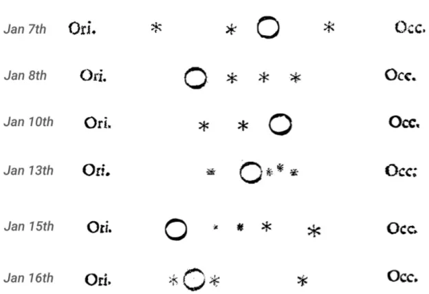
About one decade prior to his aurora observations, on January 7, 1610, Galilei made one of his first observations of the night sky with his newly invented optical instrument, the telescope. He observed Jupiter which was accompanied by three bright dots strung on a line going through the planet. He originally considered these dots as stars and sketched them together with Jupiter on a notepad (Barker 2004). Excerpts of these sketches are shown in Figure 1. During the following days, Galilei continued observing Jupiter and sketched the accompanying ”stars”.
He noticed that the observed bright dots kept their alignment on a line through Jupiter, but moved from day to day (panels 2 and 3 in Figure 1) and from hour to hour (not shown in the figure). On January 13, 1610, Galilei saw a fourth star appearing. He continued his observations until March 2, 1610, and concluded that the bright dots, which continued to change their positions relative to each other but always remained close to Jupiter, must be planetary bodies orbiting around Jupiter (Barker 2004).
Galilei published his findings in Sidereus Nuncius in 1610 (Galilei 1610), which was dedicated to his Grand Duke Cosimo de’ Medici and, therefore, he called the newly discovered moons of Jupiter the Medicean planets I, II, III and IV. This nomenclature was used for centuries until they had been renamed to the Galilean satellites Io, Europa, Ganymede and Callisto, the Greek names of the lovers of the Roman god Jupiter (Marazzini 2005). Today, we know that the Galilean satellites are the four largest moons of Jupiter among numerous small-sized and irregular moons.
1Galilei and Guiducci used the Italian term boreale aurora. It was the French scientist Pierre Gassendi (1592-1655) who introduced the Latin termaurora borealis for the first time in 1621 (Falck-Ytter and Torbjorn 1999).
CHAPTER 1. INTRODUCTION
3
Figure 1
– Galileo Galilei’s sketches of Jupiter (circle) and the Galilean satellites (stars) made in Januar 1610. ”Ori.” (abbreviation for the Latin word
orient) means East and ”Occ.” (occident) West. Each panel is taken from Galilei (1610) and is enhanced in contrast and brightness.
The homemade telescope of Galileo Galilei was a groundbreaking invention at that time and a milestone in the development of optical instruments. Of course, the accuracy of telescopes has been steadily improved over the years and centu- ries. Today, we are able to observe the Galilean satellites with a higher resolution than at Galilei’s time. With advanced spectrographs aboard space telescopes like the Hubble Space Telescope (HST) we are able to observe targets at wavelengths beyond the visible light. Due to the improvements of optical-spectroscopic instru- ments over the past decades, we discovered that the auroral outburst seen by Galilei in 1621 is not an exclusive phenomenon at Earth. Auroral emission also occurs at other planetary bodies in our solar system such as Jupiter (see, e.g., Clarke et al. (2004) and Figure 2B), Saturn (see, e.g., Kurth et al. (2009)) or Ura- nus (see., e.g., Lamy et al. (2012) and Figure 2C). The most recent observation of auroral emission on a brown dwarf (Hallinan et al. 2015; Kao et al. 2016) is the first detection of aurora on an extrasolar object outside of our solar system.
Even though the aurorae of all these planetary bodies describe the same phy-
sical phenomenon, they differ from body to body in morphology, i.e., in location,
4
CHAPTER 1. INTRODUCTIONA Aurora australis at Earth: UV false- colour image observed ny the satellite IMAGE and overlaid on an image at vi- sible wavelengths (NASA 2005).
B Aurora at Jupiter: FUV auroral oval observed with HST (NASA 1998).
C Aurora at Uranus: Composite image of HST aurora observations at visible and ultraviolet wavelengths, Voyager 2 photographs of Uranus’ disk at visible wavelengths, and Gemini Observatory observations of the Uranus’ ring system at infrared wavelengths. (NASA 2012).
D Aurora at Ganymede: The two FUV auroral ovals at frontal view on Gany- mede’s plasma downstream side, obser- ved with HST (McGrath et al. (2013), excerpt from their figure 2).
Figure 2
– Auroral ovals at Earth (A), Jupiter (B), Uranus (C) and Ganymede (D).
Note that additionally to the main oval at Jupiter the so-called footprints (indicated as
”spots” in the image) of the Galilean satellites are also visible, caused by magnetic
flux tubes which connect Jupiter’s ionosphere to the moons. The two FUV auroral
ovals at Ganymede go around the moon’s north and south pole as they do at Earth,
but at lower planetographic latitudes.
CHAPTER 1. INTRODUCTION
5
extension and shape, in brightness and in their generation processes (compare the panels in Figure 2). Today, our understanding of the physical processes of auroral phenomena is still incomplete. Generally speaking, an aurora is a light display which occurs when charged particles hit the atmosphere of a celestial bo- dy. At Earth, auroral emission mostly occurs above 60
◦latitude on the northern and southern hemisphere (Figure 2A). Originating as a stream of plasma partic- les from the sun, the solar wind interacts with the Earth’s magnetosphere. The magnetosphere is the region around a planetary body which is controlled by the body’s magnetic field. The interaction leads to an acceleration of charged partic- les (electrons and ions). These particles propagate along Earth’s magnetic field lines towards the atmosphere where they collide with neutral atoms and molecu- les (mostly oxygen and nitrogen). Due to the collisions, the atmospheric particles get excited and, after a short time, they deenergize which results in the emission of light. This emission of light is being called aurora.
In principal, three components are necessary to trigger an aurora: a generator for acceleration, accelerated charged particles and a neutral atmosphere. At Earth, the acceleration is driven by the interaction between the solar wind and Earth’s magnetic field. Another example for solar wind triggered aurora is Mars. Mars pos- sesses no global magnetic field but has only multiple magnetic field spots distri- buted over the southern hemisphere. These spots are correlated with magnetized material in the crust of the planet. In 2004, the ESA mission Mars Express dis- covered auroral emission in the far ultraviolet wavelength range (FUV) coinciding with the magnetic field spots. Although the acceleration process is still unclear, it was thought to be energetic solar wind electrons which propagate along the Martian magnetic field lines colliding with neutral gas of the Martian atmosphere (Leblanc and Chicarro 2008). However, ten years later in 2014, the NASA mission MAVEN observed auroral emission for the first time on the northern hemisphere (Phillips 2015; Brown et al. 2015). It is unclear how the solar wind interacts with the Martian atmosphere under the lack of magnetic fields on that hemisphere, but the observed aurora in that region indicates a direct interaction of solar wind particles with the neutral atmosphere.
The aurora on Jupiter demonstrates that the solar wind interaction is not a ne-
cessary condition to auroral emission. At Jupiter, the energy of the solar wind is
6
CHAPTER 1. INTRODUCTIONweaker than at Earth and the Jovian magnetic field strength is much stronger
2(Khurana et al. 2004). Since the observed aurora of Jupiter is a hundred times more energetic and ten times brighter compared to the aurora at Earth (Clarke et al. 2004), a different acceleration process has to be present. Unlike Earth’s magnetosphere, Jupiter’s magnetosphere is not dominated by the solar wind in- teraction but by the planet’s super fast rotation period of ∼10 h. Jupiter’s intrinsic magnetic field and the magnetospheric plasma roughly corotate with this rotation period at the inner part of the magnetosphere (<10 R
J, where R
J= 71,492 km is the radius of Jupiter). At the middle part of the magnetosphere (10-40 R
J) this corotation breaks down since Jupiter’s ionosphere can not transport sufficient an- gular momentum to the outflowing plasma. A radial current system develops to maintain (quasi) corotation (Khurana et al. 2004). These radial currents accele- rate electrons into the Jovian ionosphere and generate auroral ovals around both poles of Jupiter (Khurana et al. (2004); Figure 2B). This is an almost continuous process and nearly independent of the time-variable solar wind activity.
Auroral emission is not only confined to planets and their dense atmospheres, though. Aurora has been observed also on the Galilean satellites. Embedded within the Jovian magnetosphere, the velocity of the corotating Jovian magne- tospheric plasma is much higher than the orbital velocity of the satellites. The magnetospheric plasma impinges the satellites and their tenuous, neutral atmo- spheres, triggering the auroral emission. The morphology and brightness of the aurora is individual for each planet and for each satellite. They depend on the local planet- or moon-plasma interaction as well as on the composition of their atmospheres. Studying their aurora is therefore a valuable diagnostic tool for ex- ploring their magnetospheric environment and atmospheres. In this thesis, we study the morphology and brightness of the aurora on Ganymede, the largest Galilean satellite. The aurora on Ganymede shares several key features with the aurora on Earth, but there are also huge differences between the bodies besides the size and the internal composition. Both bodies have two distinct auroral ovals aligned around their north and south poles (compare Figure 2A and D; Hall et al.
(1998); Feldman et al. (2000); McGrath et al. (2013)). Unlike at Earth, where the auroral ovals can be also observed at visible wavelengths, the auroral ovals at Ganymede have been detected only in the far ultraviolet range until now. Ano-
2e.g., the equatorial magnetic field strength at Earth lies around 30,000 nT and at Jupiter at 400,000 nT (Khurana et al. 2004).
CHAPTER 1. INTRODUCTION
7
ther particularity of Ganymede is that it is the only moon known so far having its own magnetic field (Kivelson et al. 1996). This magnetic field is strong enough to maintain a region of closed magnetic field lines shielding the moon from the Jovi- an magnetic field and plasma flow in which Ganymede is embedded. This mini- magnetosphere can roughly be compared with Earth’s magnetosphere which is embedded within the solar wind. But as the Jovian magnetospheric plasma flow is sub-Alfvénic and sub-sonic, the corotating plasma can interact directly with Ganymede’s mini-magnetosphere without being modified by a bow shock, which usually forms upstream of a planetary magnetosphere like at Earth (Jia et al.
2008). Therefore, Ganymede’s mini-magnetosphere roughly forms a cylindrical shape, while Earth’s magnetosphere exhibits a bullet-like shape.
1.1 Purpose of this thesis
In the past decades, we gained a basic understanding of Ganymede’s aurora by several spacecraft missions and HST observations discussed by several authors.
The focus of this thesis is the further investigation of Ganymede’s aurora under
its time-varying components. A common feature of all Galilean satellites is that
their orbital plane and the Jovian magnetospheric equator are tilted by ∼10
◦due
to the misalignment of Jupiter’s rotation and dipole axis. As the Jovian magnetic
field corotates with the planet’s synodic rotation period of 10.5 hours, Ganymede
changes its position relative to the magnetic equator within 5.25 hours and tran-
sits through the current sheet, a thin layer with increased plasma density in the
magnetic equatorial plane. Above and below the current sheet, Jupiter’s magnetic
field orientation changes. Inside the current sheet, Ganymede is exposed to in-
creased plasma density and thermal pressure compared to outside of the current
sheet (Kivelson et al. 1997; Khurana et al. 2004). However, the influence of these
periodically changing local plasma conditions on the morphology and brightness
of Ganymede’s aurora has not been analyzed yet. We therefore analyze sets
of HST campaigns which consecutively observe Ganymede’s transit from high
elevated magnetic latitudes towards the current sheet. Due to the asymmetry of
Ganymede’s magnetosphere on the plasma upstream and downstream side, we
compare the auroral brightness on the upstream and downstream side separately
at different positions of Ganymede within the Jovian plasma sheet. We analyze
8
CHAPTER 1. INTRODUCTIONif and how the location of the ovals varies depending on Ganymede’s magnetic latitude. We also analyze the symmetry between the northern and southern oval in order to derive further constraints on the orientation Ganymede’s magnetic di- pole moment. Finally, we investigate the patchiness of the auroral emission along the ovals in order to investigate any possible correlation between the occurrence of bright auroral spots and the intermittence of the magnetic reconnection on the upstream side of Ganymede’s mini-magnetosphere.
1.2 Structure of this dissertation
First, we give in Chapter 2 a brief overview of the basic parameters of Gany-
mede such as the moon’s orbital, surface and interior parameters as well as its
intrinsic magnetic field and magnetospheric environment. We provide all infor-
mation necessary to get a basic understanding for the subsequent discussion of
Ganymede’s aurora. We present the first observations of the aurora and discuss
several theoretical works explaining the generation process of Ganymede’s auro-
ra. In Chapter 3, we introduce the HST data sets used in our analysis, the criteria
for choosing them and how they are processed. We then present and discuss
the results of our study in Chapter 4. Finally, we summarize our main findings
conclusions and give a short outlook of possible further studies in Chapter 5.
Chapter
Ganymede and the 2
discovery of its aurora
In this chapter, we present all previous observations and modeling of Ganymede’s
aurora, which are relevant for the purpose of this thesis. First, we briefly introduce
key properties of Ganymede regarding its interior and surface composition, its
atmosphere, and its subsurface ocean. We provide all necessary key features
for a basic understanding of Ganymede’s magnetospheric environment including
a description of Ganymede’s intrinsic magnetic field. In the second part of this
chapter, we discuss the discovery and all previous spectroscopic observations of
the aurora on Ganymede. At the end of this chapter, we present works by several
authors which theoretically describe the excitation process of Ganymede’s aurora.
10
CHAPTER 2. GANYMEDE AND THE DISCOVERY OF ITS AURORA2.1 Ganymede and the Jovian System
In the past decades, Ganymede, as well as the Jovian system, have been inves- tigated by several space missions including short time surveys during stop-over flybys, e.g., the Pioneer (1973/1974) and Voyager (1979) missions, as well as long time surveys. By far the longest in-situ observations were obtained by the Galileo spacecraft (1989-2003) which entered the Jovian system on December 7, 1995 and orbited Jupiter and the Galilean satellites for almost eight years. In the following, we present basic facts about Ganymede and its environment ob- tained by these space missions (supplemented by ground based observations or observations during flybys of other spacecrafts).
2.1.1 Ganymede’s surface structure, interior compo- sition, and subsurface ocean
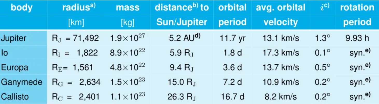
Ganymede is by far the largest moon of the Galilean satellites. Basic orbital and physical parameters of Jupiter and the Galilean satellites are summarized in Table 1 (Bagenal et al. 2004). Having a radius of R
G= 2,634 km, Ganymede not only is the largest moon among all moons of our solar system (e.g., Earth’s Moon has a radius of 1,737 km = 0.65 R
G) but is even larger than the innermost planet Mercury, which has a radius of 2,440 km (= 0.93 R
G). Being tidally locked, Ganymede takes 7 days, 3 hours and 42.6 minutes for a full rotation around Jupi- ter. Preceded by Io and Europa and followed by Callisto, Ganymede is the third of the Galilean satellites and orbits Jupiter with a low inclination 1
◦at an average distance of ∼1,070,400 km or ∼15 Jupiter radii (1 Jupiter radius R
J= 71,492 km).
The orbital velocity of Ganymede is 11 km/s and the eccentricity of Ganymede’s
orbit, 1.5 × 10
−3, is very small.
CHAPTER 2. GANYMEDE AND THE DISCOVERY OF ITS AURORA
11
Table 1
– Orbital and physical parameters of Jupiter and the Galilean satellites. (Ba- genal et al. 2004)
body radius
a)mass distance
b)to orbital avg. orbital i
c)rotation
[km] [kg]Sun/Jupiter period velocity period Jupiter R
J= 71,492 1.9 × 10
275.2 AU
d)11.7 yr 13.1 km/s 1.3
◦9.93 h Io R
I= 1,822 8.9 × 10
225.9 R
J1.8 d 17.3 km/s 0.1
◦syn.
e)Europa R
E= 1,561 4.8 × 10
229.4 R
J3.6 d 13.7 km/s 0.5
◦syn.
e)Ganymede R
G= 2,634 1.5 × 10
2315.0 R
J7.2 d 10.9 km/s 0.2
◦syn.
e)Callisto R
C= 2,401 1.1 × 10
2326.3 R
J16.7 d 8.2 km/s 0.2
◦syn.
e)a)
equatorial radius
b)
average between apo- and pericenter
c)
inclination relative to the ecliptic (for Jupiter) and Jupiter’s equatorial plane (for the moons)
d)
1 AU = 1 Astronomical Unit = 149,597,870.7 km
e)
synchronous rotation, i.e., tidally locked
Surface and albedo
The surface temperature varies between 70 K on the nightside and 152 K on the dayside. The average surface temperature is 110 K (Orton et al. 1996; Delitsky and Lane 1998). Ganymede’s surface consists mostly of frozen water but also contains minor components of carbon and sulfur dioxide (CO
2, SO
2) as well as organic compounds (McCord et al. 1998; Pappalardo et al. 2004). Most charac- teristic for Ganymede’s surface is its division into two major terrain types. Forty percent of the surface is a relatively old and dark terrain, while the rest consists of younger and brighter terrain (Showman and Malhotra 1999; Pappalardo et al.
2004). Figure 3A shows a composite image of Ganymede’s trailing hemisphere.
The false color image is a composition of images at different wavelengths taken
by the Solid State Imaging system (SSI) on board the Galileo spacecraft and
enhances the contrast between the dark and bright terrain. The dark terrain is
geologically very old and highly cratered, indicated by the white dots in Figure 3A
and 4. It contains clays and organic materials which darkens the water ice in that
terrain (Pappalardo et al. 2004). Estimated from the crater density, the dark ter-
rain is approximately four billion years old (Zahnle et al. 1998). The bright terrain
is less cratered and relatively smooth. Observations by the Galileo spacecraft
indicate that the craters in the bright area have been smoothed out due to resur-
facing, which indicates that this terrain is geologically younger than the dark ter-
12
CHAPTER 2. GANYMEDE AND THE DISCOVERY OF ITS AURORAA False color image of Ganymede’s trailing hemis- phere centered at 306◦ west-longitude (North is at the top). The image is a composition of green, vio- let, and micrometer filtered images taken on March 29, 1998 by the Solid State Imaging system on board theGalileo spacecraft.
B A 25×10 km cut-out of the trailing hemisphere (306◦ west- longitude and −14◦ latitude, North is on the right side), sho- wing parts of Nicholson Regio (top, dark terrain) and Harpa- gia Sulcus (bottom, bright ter- rain).
Figure 3
– Surface of Ganymede: Global view of Ganymede’s trailing hemisphere (A) and a zoom on Ganymede’s surface structure (B). (Pappalardo et al. 2004, supplementary material)
rain (Pappalardo et al. 2004). The bright terrain is also characterized by arrays of grooves and ridges (Pappalardo et al. 1998). Figure 3B shows the harsh contrast between the dark and bright terrain. Shown is a 25×10 km
2cut-out of Ganyme- de’s trailing hemisphere that contains parts of Nicholson Regio (top, dark terrain) and Harpagia Sulcus (bottom, bright terrain) (Pappalardo et al. 2004). The two specific regions are also indicated in Figure 4 (see blue text annotations). The mechanism for the formation of the grooved terrain is still unclear. Tectonic acti- vity is supposed as the main heating mechanism, but also cryovolcanism might have played a role for the formation of Ganymede’s surface structure (Pappalardo et al. 1998, 2004).
The mosaic of high- and mid-resolving images from the Voyager 1 and 2 and the
Galileo missions in Figure 4 provides a global view of Ganymede’s surface in the
CHAPTER 2. GANYMEDE AND THE DISCOVERY OF ITS AURORA
13
Figure 4
– Mosaic of high- and mid-resolving photographs from
Galileoand
Voyager1 and 2, mercator projected on a sphere of Ganymede’s radius for planetographic latitudes up to
±56◦(modified; for further processing details read USGS (2003)).
The planetographic central/0
◦longitude is defined by the Jupiter-facing meridian (thick vertical dashed yellow line). Leading and trailing hemispheres are also indica- ted. Names of regions on this map are approved by the International Astronomical Union (IAU). A larger version of this image is available in Figure
53in Appendix
S9.(USGS 2003)
latitudinal band between ±56
◦(USGS 2003). The brightness of each individual image is adjusted to provide a seamless composite image at visible wavelength range. We have modified the original image from USGS (2003) by adding additio- nal annotations. We indicate the central Jupiter-facing meridian, which defines the 0
◦planetographic longitude. The image uses the planetographic west-longitude system, i.e., the longitude is counted in clockwise direction. Unless otherwise in- dicated, we use this definition for Ganymede’s planetographic coordinate system throughout this work. The orbital leading and trailing hemisphere as well as their corresponding central meridian, i.e., 90
◦and 270
◦longitude, are also indicated.
In this broad overview of Ganymede’s surface, we see that the leading side seems to be brighter than the trailing side. Pappalardo et al. (2004, and references the- rein) created a global map of Ganymede’s albedo at the visible wavelength of 5600 Å (1 Å = 10
−1nm), shown in Figure 5. The authors derived a synthetic light curve (solid line) from Voyager and Galileo observations and adjusted it in order to fit various observations from ground-based
1telescope observations (circles
1i.e., Earth-based
14
CHAPTER 2. GANYMEDE AND THE DISCOVERY OF ITS AURORAFigure 5
– Albedo map of Ganymede at 5600 Å (visible light). A synthetic light curve (solid line, derived from
Voyagerand
Galileoobservations) is adjusted to various telescope observations (circles and triangles). (Pappalardo et al. (2004, their figure 16.24) and references therein)
and triangles). The light curve confirms a hemispheric albedo dichotomy for that wavelength range. Similar to Europa, the reflectance is higher on the leading side than on the trailing side (Calvin et al. 1995; Pappalardo et al. 2004). A possi- ble explanation for the dichotomy could be an enhanced reservoir of SO
2on the trailing side (Domingue et al. 1996, 1998; Pappalardo et al. 2004).
Polar caps
As frozen ice particles scatter light at shorter wavelengths, the violet enhance-
ments at the poles in Figure 3A are possibly caused by Ganymede’s frosty polar
caps (Pappalardo et al. 2004). On average, Ganymede’s polar caps have a very
vast latitudinal extension as they extend down to 40
◦latitude, at some locations
they can even reach 25
◦latitude (compared to Earth: e.g., Cologne lies at 50
◦north latitude). There are different theories about the origin of Ganymede’s polar
caps. The most common explanation is an enhanced bombardment of the surface
by plasma particles due to Ganymede’s intrinsic magnetic field, which has been
discovered by the Galileo mission (Kivelson et al. 1996; Khurana et al. 2007). The
surface sputtering leads to a redistribution of water molecules and frozen particles
can migrate into the colder areas of the polar region (Khurana et al. 2007).
CHAPTER 2. GANYMEDE AND THE DISCOVERY OF ITS AURORA
15
Interior composition
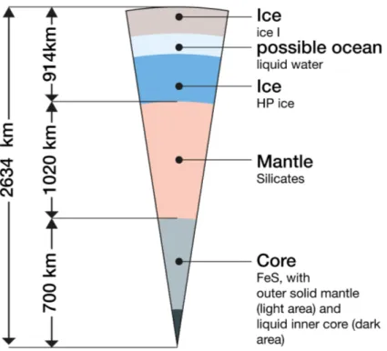
Even though Ganymede’s surface is dominated by frozen water (50–90%, Show- man and Malhotra (1999), Pappalardo et al. (2004)), its density of 1.936 g cm
−3suggests a nearly equal portion of ice and rocky material for Ganymede as a whole (Showman and Malhotra 1999). Ganymede has a mass of 1.482 · 10
23kg (Showman and Malhotra 1999). This is only 0.025 times the mass of Earth but nearly twice the mass of the Moon. Although Ganymede is slightly larger than Mercury, its mass is only half of that of Mercury. Ganymede’s moment of inertia, derived from observations during close flybys by the Galileo spacecraft, is with C/MR
22= 0.3105 ± 0.0028 the smallest measured value for a solid body in our solar system (Anderson et al. 1996; Showman and Malhotra 1999). For example, Earth has a moment of inertia of C/MR
2=0.3307 and Mercury C/MR
2=0.346. A moment of inertia lower than 0.4
3indicates an increasing density with increasing depth. The model for Ganymede’s interior by Bland et al. (2008), where Ganyme- de is differentiated into three different layers, is so far the best explanation for the measured moment of inertia. As shown in Figure 6, this model includes a central iron sulfide (FeS) core, a silicate mantle, and an outer layer of mostly frozen wa- ter. In order to sustain the intrinsic magnetic field, Showman and Malhotra (1999) suggest the existence of a metallic core and Anderson et al. (1996) and Schubert et al. (1996) propose that the radius of such a core lies between 0.15 and 0.5 R
G. In the Bland et al. (2008) model, the core has a radius of 700 km and consists of an outer solid mantle and a liquid inner core. The surrounding silicate mantle has a thickness of 1020 km. The outer layer, with a thickness of 914 km, consists of water shells of different types of ice
4and possibly one (Schubert et al. 2004) or more layers (Vance et al. 2014) of liquid water oceans of unknown thickness and depth. Possible heating sources of a subsurface ocean on Ganymede are tidal forces and the orbital resonance of Ganymede with Europa (1:2) and Io (1:4) (Showman et al. 1997). According to the model by Bland et al. (2008), the subsur- face ocean must have a minimum thickness of 22 km. In contrast, Kivelson et al.
(2002) derive a minimum thickness of 10 km from their magnetic field model. The depth of the ocean is assumed to lie between 150 and 170 km beneath the icy
2C: polar moment of inertia of the body; M: mass of the body; R: mean radius of the body.
3C/MR2 = 0.4 is the moment of inertia of a sphere with uniformly density distribution.
4In Figure6, two different types of ice are indicated: crystalline ice (ice I) and high pressure ice (HP ice). Ice is classified according to its temperature and pressure, which defines the phase state of the ice.
16
CHAPTER 2. GANYMEDE AND THE DISCOVERY OF ITS AURORAFigure 6
– Sketch of Ganymede’s interior composition according to a three-layer model by Bland et al. (2008).
surface Kivelson et al. (2002). We discuss Ganymede’s subsurface ocean in the following section in more detail.
Subsurface ocean
First indications of a subsurface ocean at Ganymede were found by Kivelson et al.
(2002) who analyzed magnetic field measurements taken by the Galileo space-
craft. However, the interpretations of these magnetometer data are not conclusi-
ve, i.e., they can be explained with two different models for Ganymede’s internal
magnetic field at the same time (Saur et al. 2015). The first model includes a
dynamo dipole field with additional quadrupole moments. The second model in-
cludes a dynamo dipole field with an induced field within a saline subsurface
ocean. In the second model, preferred by Kivelson et al. (2002), the time-variable
component of Jupiter’s magnetic field at Ganymede’s orbit is responsible for the
induction in the electrically conductive subsurface ocean. The major disadvanta-
ge of the reported magnetometer measurements is the fact that they were taken
during several flybys and the individual flyby trajectories are not identical. The-
refore, it is not possible to distinguish between spatial variations and temporal
CHAPTER 2. GANYMEDE AND THE DISCOVERY OF ITS AURORA
17
variations, i.e., between magnetic moments of higher order or induction effects in a subsurface ocean. As a consequence, the magnetic field measurements alone are ambiguous and they rather suggest than prove the existence of an ocean at Ganymede.
Saur et al. (2015) use a different approach to verify the existence of the ocean.
They analyzed the response of Ganymede’s auroral ovals to the time-varying component of the Jovian magnetospheric field in Ganymede’s vicinity. They used temporally and spatially resolved HST observations of Ganymede’s auroral ovals which do not suffer from the mentioned ambiguity of the magnetometer measurements. As sketched in Figure 7, in the absence of an ocean, Jupiter’s time-variable magnetic field would cause an oscillation of the auroral ovals by 5.8
◦± 1.3
◦(Saur et al. 2015). Saur et al. (2015) showed that the observed am- plitude of the oscillation is only 2.0
◦± 1.3
◦. As a conductive subsurface ocean partly compensates Jupiter’s time-variable fields through electromagnetic induc- tion, Saur et al. (2015) relate the reduced oscillation to the induction in a saline subsurface ocean within Ganymede. At the same time, when induction signals at Ganymede are present, the inferred quadrupole coefficients of Ganymede’s dyna- mo field must be particularly small (Kivelson et al. 2002; Christensen 2015; Saur et al. 2015). This is the first conclusive proof of a subsurface ocean by measuring the location of the auroral ovals on a solar system body. Prior to Saur et al. (2015), Roth et al. (2014b) found potential evidence for a subsurface ocean at Europa, i.e., they found erupting water vapor plumes at the moon’s surface, also by using spectroscopic HST observations
5. Saur et al. (2015) also suggest that Ganyme- de’s ocean lies between 150 and 250 km beneath the surface or, alternatively, its top edge lies at a maximum depth of 330 km.
2.1.2 Atmosphere
First indications for an atmosphere at Ganymede come from stellar experiment observation by Carlson et al. (1973). The authors estimate an atmospheric sur- face pressure of around 1 µbar
6. Observations by the Voyager Ultraviolet Science
5As the magnetospheric configuration and properties at Europa are different compared to Gany- mede, Roth et al. (2014b) used a different approach: They detected water vapor plumes above the limb of the observed disk of Europa. For more details, please read Roth et al. (2014b, a) and Roth et al. (2016).
61 microbar = 0.1 Pascal (Pa) = 0.1 N m−2
18
CHAPTER 2. GANYMEDE AND THE DISCOVERY OF ITS AURORAocean
ocean nooceannoocean rocking of the
oval within 5.2 h rocking of
magnetospheric field within 5.2 h
Jupiter OCFB
Figure 7
– Sketch of the ”rocking” auroral ovals at Ganymede taken from Saur et al.
(2015, their figure 1). Within 5.25 hours, Ganymede transits from above to below the Jovian current sheet and experiences a change of orientation of the Jovian ma- gnetospheric field (simplified, blue thin lines). Shown is the case when Ganymede is above (dashed lines) and below the current sheet (solid lines), respectively. The auroral ovals, whose location coincide with the location of the open-closed field line boundary (OCFB, further details see Section
2.1.3), respond to this time-varyingmagnetic field by a ”rocking”, i.e., an oscillation of the ovals. Without induction in a subsurface ocean this oscillation is stronger (blue lines) than with induction (red lines) as the induction in an ocean partly compensates Jupiter’s time-variable field.
telescope (UVS) five years later could not confirm an atmosphere and placed an
upper limit on the surface pressure. This value is five times lower in magnitude
than the value suggested by Carlson et al. (1973) and corresponds to a surface
particle number density of 1.5 × 10
9cm
−3(Broadfoot et al. 1981). Around two
decades later, Hall et al. (1998) finally find new evidence for an atmosphere on
Ganymede from spectroscopic Hubble Space Telescope Goddard High Resoluti-
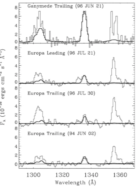
on Spectrograph (HST/GHRS) observations. Hall et al. (1998) observe emission
at the FUV wavelengths at OI λ1304 Å and OI λ1356 Å (Figure 13) which is as-
sociated to an airglow of atomic oxygen. The excitation of this airglow, in turn, is
associated with dissociation of neutral molecular oxygen by electron impact, indi-
cating that a tenuous neutral oxygen atmosphere must be present at Ganymede.
CHAPTER 2. GANYMEDE AND THE DISCOVERY OF ITS AURORA
19
Figure 8
– Heating map of Ganymede’s dayside from Orton et al. (1996, their figure 1; reprinted with permission from AAAS, see Appendix
S9for further details). Top axis is in Ganymede local time (e.g., 12 h = local noon), bottom axis is in plane- tographic west-longitude.
y-axis is in planetographic latitudes. Color coded is thetemperature range from 90 to 150 K.
Implied from the intensity ratio of the two oxygen lines, this atmosphere predomi- nantly consists of molecular O
2(Hall et al. 1998). Hall et al. (1998) calculate an O
2column density lying between 10
14and 10
15cm
−2.
Two sources for Ganymede’s atmosphere are suggested: sublimation and sputte- ring of the frozen water on the surface (Eviatar et al. 2001b; Turc et al. 2014).
Sublimation is predominant in the region around the sub-solar point, i.e., the equatorial and tropical region on the dayside. Here, water vapor and hydroxyl (HO) are able to survive in the atmosphere (Eviatar et al. 2001b). Since this re- gion is shielded from magnetospheric energetic electrons by closed field lines of Ganymede’s magnetic field, photodissociation is the main process for splitting the water molecules into hydrogen and oxygen (Budzien et al. 1994; Eviatar et al.
2001b). The volatile hydrogen escapes the atmosphere due to the low energy,
which is required to escape from Ganymede’s surface (Eviatar et al. 2001b). The
heavier oxygen remains gravitationally bound to Ganymede, forming the atmo-
sphere. Atomic oxygen is created by photodissociation of O
2molecules (86%)
and H
2O (14%) (Eviatar et al. 2001b). In the polar region and on the nightside,
20
CHAPTER 2. GANYMEDE AND THE DISCOVERY OF ITS AURORAthe temperatures are too low for sublimation (Eviatar et al. 2001b; Turc et al.
2014) as shown in Figure 8 (taken from Orton et al. (1996)). The heating map for Ganymede’s dayside in Figure 8 shows a vast temperature gradient from ∼ 150 K around the subsolar point to ∼ 90 K at higher latitudes and in the pre-dawn region (Orton et al. 1996). O
2, H
2and H are produced by sputtering of surface water ice in the magnetospheric unprotected polar region, i.e., the region of open magnetic field lines without magnetospheric shielding effects (Bar-Nun et al. 1985; Eviatar et al. 2001b). Sputtered water vapor and OH recondense at once in the low tem- perature region at the poles and nightside. The hydrogen (atomic and molecular) escapes rapidly, again due to the low escape velocity required at Ganymede. On- ly molecular oxygen can survive in gaseous state at temperatures above 80 K (Johnson 1996) forming the atmosphere in these colder regions (Eviatar et al.
2001b).
The two different atmospheric production processes lead to a strong atmospheric dichotomy between polar and subsolar equatorial regions (Turc et al. 2014). This atmospheric dichotomy also impacts Ganymede’s ionosphere. The existence of an ionosphere at Ganymede is implied by its indigenous, neutral atmosphere as neutral oxygen (atomic and molecular) gets ionized by magnetospheric energe- tic electrons and solar extreme ultraviolet (EUV) radiation (Paranicas et al. 1999;
Eviatar et al. 2001b). Eviatar et al. (2001b) report that the ionosphere is domi- nated by molecular oxygen ions in the polar and by atomic oxygen ions in the equatorial region. In addition to the ionospheric plasma outflow, i.e., an outflow of oxygen ions at the polar caps, Eviatar et al. (2001b) expect an oxygen corona above the limb of Ganymede from neutral, (low) excited oxygen atoms escaping the polar cap region. A corona of escaping hydrogen has been already detected by Feldman et al. (2000) with the Space Telescope Imaging Spectrograph (STIS) on board of HST. Feldman et al. (2000) actually confirmed the previous discovery of a Lyman-α emission from a hydrogen exosphere by Barth et al. (1997) from Galileo UVS observations.
2.1.3 Ganymede’s intrinsic magnetic field and ma- gnetospheric environment
One major finding of the Galileo mission regarding Ganymede is the discovery
of the intrinsic magnetic field of the moon (Kivelson et al. 1996). So far, Gany-
CHAPTER 2. GANYMEDE AND THE DISCOVERY OF ITS AURORA
21
mede is the only known moon which possesses its own permanent magnetic field embedded within a planetary magnetosphere. The magnetic field is strong enough to shield Ganymede from the Jovian magnetic field and a so-called mini- magnetosphere develops. In the following, we briefly describe the individual com- ponents of Ganymede’s magnetic field and its interaction with the surrounding Jovian magnetic field.
Discovery and main characteristics
From magnetic field measurements by the Galileo spacecraft during the six clo- se flybys at Ganymede, G1
7, G2, G7, G8, G28 and G29, from 1996 to 2000, Ganymede’s magnetic field topology has been analyzed at significant different locations in the magnetospheric environment of the moon. In first-order, Gany- mede’s magnetic field can be approximated by a dipole magnetic field (Kivelson et al. 1996, 1998) with an equatorial field strength of 719 nT
8(Kivelson et al.
2002). The magnetic moment of the dipole is tilted by 176
◦, i.e., the magnetic north pole lies in the southern hemisphere and is rotated by −24
◦planetographic west-longitude (Kivelson et al. 2002). Higher moments, e.g., quadrupole moments are very small compared to the dipole moment (Kivelson et al. 2002).
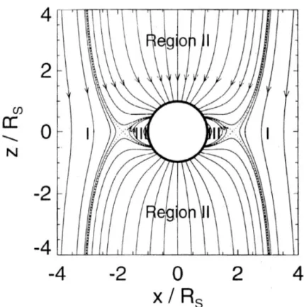
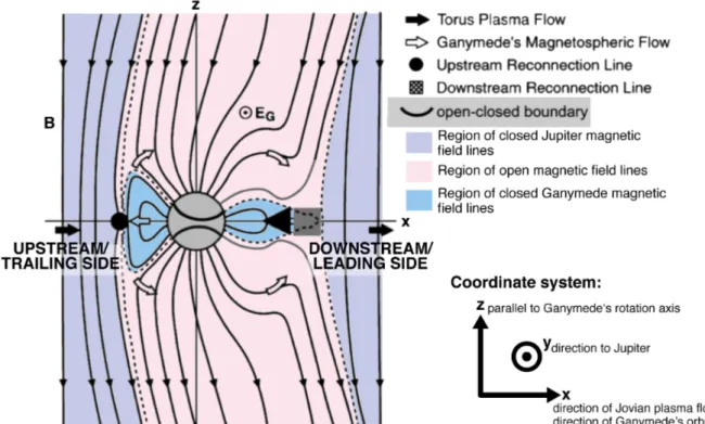
Shortly after the discovery of Ganymede’s magnetic field, Kivelson et al. (1996) developed a first-order approximation of the magnetic field topology at Ganyme- de. Adopted by Neubauer (1998), this simplified model is shown in Figure 9. It consists of a vacuum-superposition of Ganymede’s magnetic dipole field and the ambient Jovian background magnetic field (both fields are oriented in anti-parallel direction). Even though this model neglects the local plasma interaction and in- ternal induced fields, it demonstrates very well the different magnetospheric re- gions emerging at Ganymede. Region I is defined by the closed magnetic field lines starting and ending in the ionosphere of Jupiter. Open field lines at the po- les connect Ganymede with the Jovian ionosphere and define Region II. Finally, Region III is defined by the region of closed Ganymedean field lines around Ga- nymede’s equator, i.e., they start and end on Ganymede. The open-closed field line boundary (OCFB), sometimes also called separatrix, separates the individual regions from each other.
7the number refers to the orbit of the close flyby at Ganymede
81 Tesla (T) = 1 kg s−2A−1
22
CHAPTER 2. GANYMEDE AND THE DISCOVERY OF ITS AURORAFigure 9
– First-order approximation of the magnetic field topology at Ganymede (taken from Neubauer (1998)): A vacuum-superposition of a parallel Ganymedean dipole magnetic field and ambient Jovian background magnetic field. Viewing geo- metry see Figure
10. RSis the radius of Ganymede. Region
Ito
IIIindicate the region of closed field lines originating and ending on Jupiter (I), open field lines connecting Ganymede with the Jovian ionosphere (II) and closed Ganymedean field lines (III), respectively.
As the background magnetic field of Jupiter at Ganymede’s orbit with 120 nT is low compared to Ganymede’s equatorial field strength, Ganymede’s intrinsic magnetic field is strong enough to carve out space in the Jovian magnetosphe- re, creating a so-called mini-magnetosphere around Ganymede with a diameter between 4 to 5 R
G(Kivelson et al. 1998; Neubauer 1998). In agreement with Ga- nymede’s oxygen atmosphere (see Section 2.1.2), the main ion species of this mini-magnetosphere are O
+and O
+29(Eviatar et al. 2001b). At Ganymede’s ma- gnetic equator, both, the Jovian and Ganymedean magnetic field, are oriented in anti-parallel direction and magnetic reconnection might occur at points where both fields intersect (Neubauer 1998).
On its orbit around Jupiter, Ganymede always remains in the Jovian magnetos-
9The low latitude region is dominated by O+, while in the polar cap region the main ion species are O+and O+2(Eviatar et al. 2001b).
CHAPTER 2. GANYMEDE AND THE DISCOVERY OF ITS AURORA
23
Figure 10
– Schematic view of Ganymede’s magnetic field taken from Kivelson et al.
(2004, their figure 21.4, modified), viewing onto the two-dimensional plane which contains the Jovian plasma flow and Ganymede’s orbital trajectory (x-direction) and Ganymede’s rotation axis (z-direction). The view points into the direction towards Jupiter (y-direction, not shown here, see coordinate system definition for further details). Indicated are the three different magnetic field lines regions: closed field lines originating and ending on Jupiter (violet), open field lines connecting Gany- mede with the Jovian ionosphere (red) and closed Ganymedean field lines starting and ending on Ganymede (blue). The open-closed field boundary (OCFB, dashed line) separates the individual regions form each other. The OCFB’s intersection with Ganymede’s surface/ionosphere is sketched as the two thick curves on the moon disk.
phere. Furthermore, Ganymede is exposed to the steady flow of the Jovian ma-
gnetospheric plasma. At Ganymede’s orbit, the plasma flow slightly sub-corotates
with the Jovian magnetic field with a flow velocity of 150 km/s which is much hig-
her than Ganymede’s orbital velocity of 11 km/s (Kivelson et al. 1998, 2002; Mc-
Grath et al. 2013). Hence, Ganymede is constantly overtaken by the bulk plasma
flow. The plasma impinges the upstream side, i.e., Ganymede’s trailing hemisphe-
re, and distorts the dipolar shape of Ganymede’s magnetosphere. This forms the
bullet-like shape which can be observed for many other planetary magnetosphe-
res in the solar system like at Earth, where the solar wind hits and distorts Earth’s
magnetosphere in the same way. Unlike at Earth, where the incoming plasma flow
is super-sonic, the bulk plasma flow at Ganymede is sub-sonic and no bow shock
24
CHAPTER 2. GANYMEDE AND THE DISCOVERY OF ITS AURORAforms on the upstream side. Under these circumstances, Ganymede’s magneto- sphere has a more cylindrical shape rather than the typical bullet-like shape.
In addition to the simple vacuum-superposition shown in Figure 9, Figure 10 shows Ganymede’s magnetic field environment under the influence of the im- pinging plasma flow. We have modified this figure from Kivelson et al. (2004, their figure 21.4) and indicated the three different magnetospheric regions from abo- ve with colors: closed Jovian magnetic field lines (violet shaded area), open field lines connecting Ganymede with Jupiter’s ionosphere (red) and the region of clo- sed Ganymedean field lines (blue). The plasma flow velocity is in x-direction and the z-axis contains Ganymede’s rotation axis. The viewer looks into the direc- tion towards Jupiter (see coordinate system definition in that figure for a better understanding). The OCFB is indicated by the dashed line. The OCFB’s intersec- tion with Ganymede’s surface is sketched as the two thick curves on the moon disk. The points of reconnection are actually points where two separatrices inter- sect (indicated by a black circle and square in that figure). In a three-dimensional interpretation, the reconnection points form a ring surrounding Ganymede (Neu- bauer 1998; Duling et al. 2014). Figure 10 also demonstrates the influence of an additional magnetic field due to the plasma interaction (Kopp and Ip 2002; Ip and Kopp 2002; Jia et al. 2009b). On the upstream side, this additional magnetic field is oriented anti-parallel to the ambient Jovian magnetic field and counter- acts the background field, i.e., it weakens the background magnetic field. Due to the slight weakening of the background magnetic field, Ganymede’s intrinsic field becomes more effective and is able to expand the mini-magnetosphere on the upstream side. This expansion leads to a shifting of the OCFB towards higher latitudes on Ganymede. On the downstream side, the opposite is the case and the mini-magnetosphere gets stretched into the plasma flow direction and hence the OCFB shifts down towards lower planetographic latitudes.
Origin of the intrinsic magnetic field
Overall, Ganymede’s magnetic field consists of a superposition of the satellite’s
intrinsic magnetic field, the Jovian background field, the induced field in a subsur-
face ocean (see Chapter 2.1.1), and the magnetic field due to the local plasma
interaction. Ganymede’s magnetosphere and its interaction with the local plasma
has been modeled by several authors, e.g., Kivelson et al. (2002), Kopp and Ip
CHAPTER 2. GANYMEDE AND THE DISCOVERY OF ITS AURORA
25
(2002), Ip and Kopp (2002), Paty and Winglee (2004), Jia et al. (2008), Jia et al.
(2009b) and Duling et al. (2014). These theoretical works were able to reproduce and explain the Galileo magnetic field measurements. In contrast, the origin of the measured Ganymedean magnetic field is still controversially discussed. For example, Crary and Bagenal (1998) suggest remanent ferromagnetism hold in an outer layer which is enriched with iron-bearing minerals and magnetite. The sour- ce of this remanent ferromagnetism would be Jupiter’s magnetic field in the past, when Ganymede was closer at Jupiter, or a paleomagnetic field originating from a dynamo which would have become inactive today. On the other hand, due to the measured weak quadrupole moments, Kivelson et al. (2002) suggest a con- vectively driven dynamo in Ganymede’s liquid iron-sulfide (FeS) core (Figure 6).
Additional contribution to the dynamo driven magnetic field comes from the so- called iron snow (Zhan and Schubert 2012; Christensen 2015). On top of the core, liquid iron crystalizes as the core temperature decreases below the melting tem- perature of iron. The solidified iron becomes heavier than the surrounding liquid iron and sulfur and sinks down to deeper core regions. At deeper core regions, the temperature increases and the iron snow remelts again and enriches the core fluid with iron, driving compositional convection (Christensen 2015).
Variability of the magnetospheric environment
The Jovian magnetic field can be described in a first-oder approximation as a di-
pole magnetic field (Krupp et al. 2004). Its dipole moment is tilted by 9.6
◦relative
the rotation axis. A simplified representation of the Jovian magnetospheric field
lines is shown in Figure 11 after the model by Engle (1992). Shown is the periodi-
cal variation of the Jovian magnetic field orientation relative to Jupiter’s equatorial
plane within 10.5 hours, the synodic rotation period of Jupiter. This global model
of the Jovian magnetosphere includes a thin current sheet layer constrained to
the dipole magnetic equator (not shown in the figure). The current sheet (CS),
also called plasma sheet, is a layer of magnetospheric plasma which is constrai-
ned to the magnetic equator due to centrifugal forces from the corotating plasma
(Khurana 1997; Khurana et al. 2004). However, Engle (1992)’s model does not in-
clude hinging and delaying of the current sheet due to internal and external forces
on the Jovian magnetic field configuration (Khurana et al. 2004). Figure 12 shows
a more realistic geometry of the current sheet after Khurana et al. (2004).
26
CHAPTER 2. GANYMEDE AND THE DISCOVERY OF ITS AURORAA Magnetic dipole axis tilted 10◦ towards the sun.
B Magnetic dipole axis tilted 10◦ away from the sun.
Figure 11
– Two-dimensional noon-midnight plane (positive
x-direction points to-wards the sun) of Jovian magnetic field lines after Engle (1992, their figures 2 and 3) for two different magnetic field orientations relative to Jupiters rotation axis/equatorial plane.
Figure 12