The U.S. consumption-wealth ratio and foreign stock markets: International evidence for return predictability

The U.S. consumption-wealth ratio and foreign stock markets: International evidence

for return predictability

Thomas Nitschka

Department of Economics, University of Dortmund D-44221 Dortmund, Germany

E-mail: T.Nitschka@wiso.uni-dortmund.de Web: http://www.wiso.uni-dortmund.de/~ae-thni/

Phone: +49-(0)231-755-3266 JEL classi…cation: E21, G12

Keywords: Cointegration, Consumption-wealth ratio, Stock return predictability

January 2006

Abstract

A simple manipulation of the cointegrated framework proposed by Lettau and Ludvigson (2001, 2004) allows to demonstrate that temporary ‡uctua- tions of the U.S. consumption-wealth ratio predict excess returns on interna- tional stock markets. This …nding is the re‡ection of an important common, temporary component in international stock markets and thus provides em- pirical evidence for a robust link between stock markets at business cycle frequency. Moreover, I …nd that between one third and more than a half of the covariation of long-horizon returns on the G7 stock markets is explained by the common transitory stock market component identi…ed in this paper.

Furthermore, U.S. households seem to rebalance their foreign equity portfo-

lio in response to the perception of local currency rather than exchange rate

adjusted returns.

1 Introduction

Long-term predictability of asset returns is by now well documented in a growing body of empirical literature.

This paper contributes to this litera- ture by employing the framework proposed by Lettau and Ludvigson (2001, 2004) to explore the cyclical link between international stock markets.

Lettau and Ludvigson (2001, 2004) show that ‡uctuations of the U.S.

consumption-wealth ratio, the residual of the cointegration relation between consumption and aggregate wealth, predict real and excess returns on broad U.S. stock indexes. Using the Lettau and Ludvigson framework, Fernandez- Corugedo et al. (2003), Fisher and Voss (2004) and Tan and Voss (2003) pro- vide evidence for the forecast ability of the UK and Australian consumption- wealth ratio for excess returns on respective national stock indexes. Hamburg et al. (2005) …nd that German stock market returns are not predicted by variations of the national consumption-wealth ratio which seems to be the consequence of limited stock market participation of German households.

Apart from the special case of Germany, consumption-wealth ratios of Anglo-Saxon countries predict excess returns on national stock markets and thus corroborate theoretical macroeconomic models which argue that time variation of stock returns is due to cyclically varying risk premia. Fluctu- ations of risk premia over time result from agents´ time-varying risk aver- sion over the business cycle induced by the formation of consumption habits (Campbell and Cochrane, 1999) or the presence of uninsurable background risks (Constantinides and Du¢ e, 1996; Heaton and Lucas, 2000 a, b).

But despite macroeconomic explanations of stock return predictability and evidence of strong comovement between national stock markets since the mid-eighties (Brooks and Del Negro, 2005), a robust link between stock markets at business cycle frequency seems hard to capture. Furthermore, it is not even clear how comovement of stock markets can be rationalized. Do international stock markets follow a common stochastic trend as argued by Kasa (1992) or is comovement rather the outcome of a common stationary component in stock prices? Richards (1995) weakens the basis of Kasa´s statistical evidence which gives place for scepticism regarding evidence of a common stochastic trend among international stock markets. However, so far the literature also lacks convincing evidence of a common stationary component in stock markets.

1

see Cochrane (2005) for an excellent survey

In this paper I argue that the cointegration framework proposed by Let- tau and Ludvigson (2001, 2004) has the potential to shed light on this is- sue. Based on the idea that transitory ‡uctuations of wealth leave consump- tion una¤ected, Lettau and Ludvigson provide evidence that mainly tran- sitory market value changes of U.S. households´ stock holdings cause the U.S. consumption-wealth ratio to ‡uctuate temporarily. These market value changes are induced by the expectation of time-varying stock returns which explains the predictive power of short-run variations of the U.S. consumption- wealth ratio for excess returns on the U.S. stock market. U.S. households´

stock market wealth is a prime example of the home bias in equity portfolios (Tesar and Werner, 1995). Nevertheless, U.S. households hold either directly or indirectly foreign stocks which amounts to a relatively small part of U.S.

households´ stock market wealth, but inevitably raises the question if the explanation for the predictive power of the U.S. consumption-wealth ratio for the U.S. stock market also pertains to foreign stock markets.

I deal with this issue by using a simple manipulation of the Lettau and Ludvigson framework to show that variation in the market value of U.S.

households´ foreign equity holdings is induced by the expectation of time- varying returns on foreign stock markets. Hence, temporary variations of the U.S. consumption-wealth ratio predict excess returns on international stock markets. These …ndings leave the impression that the ratio of consumption to aggregate wealth in the U.S. re‡ects a common, temporary component in international stock markets. I present evidence that between one third and more than a half of the covariation of long-horizon returns on G7 stock in- dexes can be attributed to the common, transitory stock market component.

Furthermore, exchange rate changes are not predictable by variations of the U.S. consumption-wealth ratio which conveys the notion that ex- change rate changes do not cause the cyclical market value variation in U.S.

households’ foreign equity holdings. This …nding underlines that the U.S.

consumption-wealth ratio echoes a common stock market component.

Additionally, I provide evidence that U.S. households rebalance their eq- uity portfolio in response to the perception of time variation in expected local currency returns rather than to exchange rate adjusted returns.

The remainder of this paper is organised as follows. The theoretical frame-

work is introduced in section two. Section three discusses the cointegration

and error correction properties of my U.S. consumption-wealth ratio approx-

imation in detail. Section four identi…es permanent and transitory shocks in

the cointegrated system and reports variance decompositions of the cointe-

grated variables with respect to these shocks. Section …ve provides details about long-horizon regressions of changes of U.S. households´ foreign equity holdings and excess returns on foreign stock indexes on the cointegration residual. Section six gives evidence for the robustness of the long-horizon re- gressions and quanti…es to what extent the common stock market component is responsible for the covariation of long-horizon returns on G7 stock mar- kets. Section seven concludes. The appendix contains a detailed description of data employed in this paper.

2 The Consumption-Wealth Ratio

I follow Lettau and Ludvigson (2001,2004) as well as Campbell and Mankiw (1989) and consider a representative agent economy in which all wealth is traded. The representative household faces an intertemporal budget con- straint of the form

W

= (1 + R

)(W

C

) (1) where W

denotes aggregate wealth (human wealth plus asset wealth) in period t, C

; consumption and R

the net return on aggregate wealth.

Rearranging the budget constraint for the ratio of consumption to wealth and taking a loglinear approximation around the mean consumption-wealth ratio under the assumption that this mean is covariance stationary leads to the following law of motion for the log consumption-wealth ratio.

c

w

= E

X

i=1 i

w

(r

c

) (2)

Lower-case letters denote natural logarithms throughout the paper, rep- resents the di¤erence operator. In order to make (2) empirically tractable, Lettau and Ludvigson (2001, 2004) decompose aggregate wealth into its com- ponents asset and human wealth and loglinearise around the long-run mean of the ratio of human and asset wealth which leads to

w

va

+ (1 v)h

(3)

with v interpretable as average share of asset wealth in aggregate wealth, a

,

log asset wealth and h

, log human wealth. I further decompose asset wealth

into foreign equity held by U.S. households and the rest of asset wealth which

I will refer to as domestic asset wealth. A loglinear approximation of asset wealth around the foreign equity to domestic asset wealth ratio yields

a

f e

+ (1 )daw

(4)

with the average share of foreign equity in U.S. households´ asset wealth, f e

, foreign equity and daw

, domestic asset wealth.

Combining (3) with (4) gives

w

f e

+ daw

+ (1 )h

(5)

where = v is the average share of foreign equity in aggregate wealth and

= v(1 ) the average share of domestic asset wealth in aggregate wealth.

A loglinear approximation of the gross return on asset wealth with respect to foreign equity and domestic asset wealth combined with the loglinear proxy of the return on aggregate wealth decomposed into asset wealth and human wealth

gives

r

= r

+ r

+ (1 )r

(6)

Plugging (6) and (4) into (2) and taking expectations on both sides of the equation yields

c

f e

daw

(1 )h

(7)

= E

f X

i=1 i

w

[( r

+ r

+ (1 )r

) c

] g

However, (7) cannot be employed for empirical purposes because one part of aggregate wealth, human wealth, is unobservable. I assume labour income to represent the dividend paid from human wealth and thus its non-stationary component to overcome this obstacle. Then log human wealth, h

; obeys

h

= + y

+ z

(8)

with, y

, log labour income, , a constant term and a covariance stationary term z

. Plugging (8) into (7) and assuming that the net return on labour income equals the net return on human wealth gives

2

see Campbell (1996) for details

c

f e

daw

(1 )y

(9)

= E

f X

i=1 i

w

[( r

+ r

+ (1 ) y

) c

] + (1 )z

g

According to (9) c

, log consumption, f e

, log foreign equity, daw

, log domestic asset wealth and y

, log labour income cointegrate, provided they are integrated of order one, I(1). Hence, time variation of the consumption- wealth ratio, i.e. a temporary deviation from the common trends, mirrors ei- ther changes of (returns on) foreign equity, returns on domestic asset wealth, changes of labour income or consumption growth, or an arbitrary combina- tion. Furthermore, estimates of the cointegration coe¢ cients should re‡ect

; and (1 ), the average shares of the wealth components in total wealth.

2.1 Empirical evidence: Cointegration and error cor- rection

In this section, I assess the cointegration properties of my loglinear proxy of the U.S. consumption-wealth ratio. All variables are quarterly, per capita, real in billions of chain-weighted 2000 U.S. dollars and transformed to natural logarithms for the sample period from second quarter 1952 to second quarter 2004.

As pointed out by Lettau and Ludvigson (2001) as well as Rudd and Whe- lan (2002), the budget constraint (1) refers to total personal consumption

‡ows. Since we do not observe consumption ‡ows we rely on expenditures as best proxy. I thus follow Blinder and Deaton (1985) and approximate log total consumption expenditure as constant multiple of log non-durables and services consumption expenditure excluding clothing and shoes.

Rudd and Whelan (2002) provide evidence that the linear relation be-

tween log non-durable and services consumption and log total personal con-

sumption expenditure is not constant over time. However, Lettau and Lud-

vigson (2004) argue that durable consumption expenditure represents rather

replacements or additions to an existing stock than a service ‡ow from the

stock of durable goods and hence is better described as wealth which is the

view I follow in this paper. Furthermore, Rudd and Whelan cast doubt on the

appropriateness of using di¤erent de‡ators to obtain real variables. Lettau

and Ludvigson use the de‡ator for total personal consumption expenditure to de‡ate their asset wealth and labour income proxy but a di¤erent de‡ator for their consumption approximation. I take this critique into account and de‡ate all variables with the CPI of total personal consumption expenditure.

Labour income is proxied as proposed by Lettau and Ludvigson (2001, 2004). U.S. households´ foreign equity holdings are determined as explained in detail in the appendix. Domestic asset wealth is household net worth less foreign equity holdings.

Unit root tests provide evidence that each variable employed in this analy- sis contains a unit root. In addition, I cannot reject that …rst di¤erences of the variables under consideration are stationary.

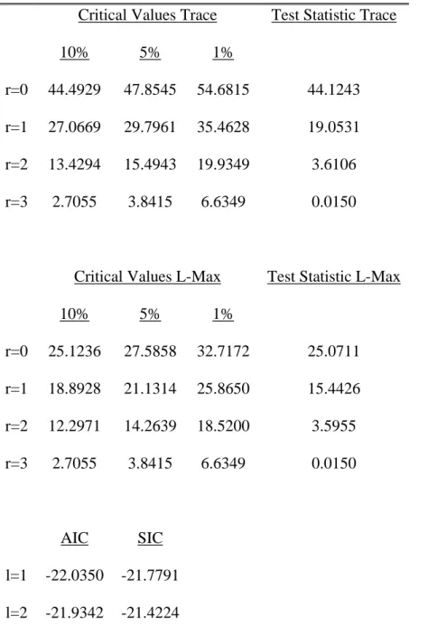
Non-durable consumption, foreign equity, domestic asset wealth and labour income are I(1), which con- veys the notion that my four-variable approximation of the log consumption- wealth ratio should cointegrate. Table 1 displays results of the Johansen cointegration test, critical values for Trace and L-max test as well as the test statistics for both of the tests. Akaike (AIC) and Schwartz (SIC) information criteria suggest an appropriate lag length of one quarter for the vector au- toregressive representation (VAR) of the four variables. According to the test statistics, I cannot reject the null of no cointegration for the relation between non-durables and services consumption expenditure excluding clothing and shoes, foreign equity holdings, domestic asset wealth and labour income at 90 percent con…dence level.

However, Ho¤mann and Mac Donald (2003) point out that the existence of a cointegrating relationship cannot be only grounded on statistical devices but should incorporate economic theory. Furthermore, theory suggests that the estimates of the cointegration coe¢ cients should re‡ect the average share of the respective wealth component in total wealth. I impose one cointegrat- ing relationship on consumption, foreign equity, domestic asset wealth and labour income and estimate the cointegration vector to investigate this point.

As emphasized by Stock (1987), OLS estimates of cointegrated variables converge to their true value with the sample size rather than with the square root of the sample size. Thus, these estimates are "superconsistent" and simple OLS provides consistent point estimates. But the error terms of the individual time-series variables could be correlated with each other. Hence,

3

Results are not reported but available upon request.

4

Philipps-Ouliaris cointegration test as well as the cointegration test by Shin provide

qualitatively similar results which are not reported but available from the author upon

request.

the OLS estimates are consistent but potentially biased away from the true values.

That is why I follow Stock and Watson (1993) who propose a dynamic least squares technique to overcome this obstacle which is in this context achieved by adding leads and lags of …rst di¤erences of foreign equity, do- mestic asset wealth and labour income as additional regressors in a regression of consumption on the level of the three wealth components. The estimate equation takes the following form:

c

= +

f e

+

daw

+

y

(10)

+ X

i= k

b

f e

+ X

i= k

b

daw

+ X

i= k

b

y

+ "

Estimation of the cointegration coe¢ cients

with i = f e; daw; y gives b

if the coe¢ cient on non-durable consumption is normalized to unity with t-statistics in parenthesis.

The coe¢ cients of di¤erences in lead or lag are omitted.

b

= [1 0:0106

(2:8954)

f e

0:3409

(8:9507)

daw

0:7331y

]

At …rst glance, the estimated cointegration coe¢ cients of foreign equity holdings, domestic asset wealth and labour income do not seem to be eco- nomically meaningful as they sum to a number bigger than unity. However, Ho¤mann (2005) provides an explanation for this …nding. Equation (10) is derived from the budget constraint (1) which refers to total consumption. I assume total personal consumption expenditure to be a constant multiple of non-durables and services consumption, i.e. total personal consumption less consumption expenditure of durable goods on the left hand side of (10). But the stock of durables is included in the asset wealth proxy on the right hand side of the estimate equation such that the estimates should sum to a number larger than one. Estimation of the cointegration vector using total personal consumption instead of non-durables and services consumption expenditure

5

The estimates do not vary much from one to seven leads and lags. Here six leads

and lags are employed. Johansen´s maximum likelihood procedure provides very similar

estimates.

leads to the cointegration vector b

. b

= [1 0:0132

(2:8860)

f e

0:2296

(8:9216)

daw

0:7684y

]

Note that the cointegration coe¢ cient estimates of foreign equity and labour income remain relatively stable whereas the coe¢ cient of domestic asset wealth less the stock of durable goods decreases. The sum of the wealth cointegration coe¢ cients is now almost exactly unity.

If non-durable and services consumption expenditure is used as consump- tion proxy, then the sum of the wealth cointegration coe¢ cients increases by eight percent to 1.08. An interpretation of this …nding is that the present value of durable consumption amounts to eight percent of the present value of total consumption. Hence, estimates of the cointegration vector employing non-durable consumption expenditures should mirror that in the long-run the net present value of asset wealth including the stock of durable goods ex- ceeds the present value of non-durable consumption by approximately eight percentage points. This argument is consistent with the respective cointe- gration coe¢ cient estimates of asset wealth inclusive and exclusive the stock of durable goods.

Furthermore, the Federal Reserve Board of Governors reports replacement costs of durable goods in household net worth. The share of durable goods in household net worth is around eight to nine percent on average over the sample period which further supports the reasoning from above.

The point estimate of the foreign equity cointegration coe¢ cient is rea- sonable as well, i.e., it mirrors the average share of foreign equity in total wealth over the sample period from 1952 to 2004.

Based on the economically meaningful cointegration coe¢ cient estimates, I assume the presence of one cointegrating relationship between the four variables under consideration throughout the paper.

I thus proceed to assess the error correction properties of the cointegrated system with non-durable and services consumption expenditure as consump- tion proxy to examine if foreign equity adjusts a temporary deviation from the common trend among consumption and aggregate wealth. I exploit that for every cointegrating relation an error-correction representation exists (En- gle and Granger (1987)).

The vector error correction representation (VECM) of x

= (c

; f e

; daw

; y

)

is

(L) x

= b

x

+ "

(11) in which x

= ( c

; f e

; daw

; y

)

is the vector of …rst di¤erences and x

the vector of lagged levels, = (

;

;

;

)

represents the vector of error correction coe¢ cients. (L) denotes a (4 by 4) matrix poly- nomial in the lag operator and b = (1; b

; b

; b

)

is the vector of the above estimated cointegration coe¢ cients when non-durable and ser- vices consumption expenditure is used as consumption proxy. Hats indicate estimated variables and "

represents the (4 by 1) vector of shocks in the cointegration relation with covariance matrix . Lower-case letters in bold face denote vectors, bold upper-case letters represent matrices.

The term b

x

gives the cointegration residual, is the adjustment vector that displays what variables adjust a deviation from the common trend among consumption and wealth. If x

is cointegrated, at least one of the adjustment coe¢ cients

;

;

or

must take values di¤erent from zero in the error-correction representation.

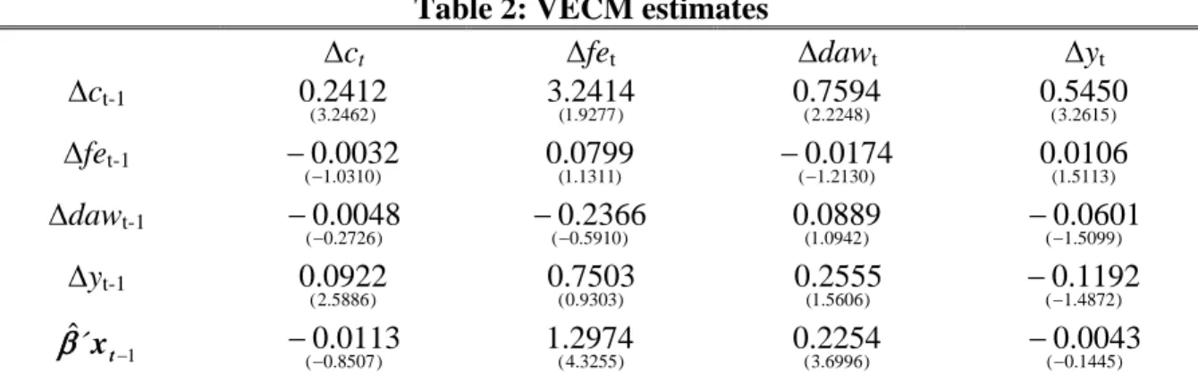
Table 2 reports VECM coe¢ cient estimates. The lag length of one has been chosen according to Akaike and Schwartz information criteria. T- statistics of the coe¢ cient estimates are in parenthesis. I focus on the ad- justment coe¢ cients in the last row of table 2.

The adjustment coe¢ cient estimates of both asset wealth components are statistically di¤erent from zero which mirrors the responsibility of asset wealth for the error correction in the cointegrated system. Domestic asset wealth adjusts temporary deviations from the common trend between con- sumption and total wealth which is presumably driven by the domestic stock market wealth component (Lettau and Ludvigson, 2004).

In addition, the adjustment coe¢ cient of foreign equity is not only statis-

tically signi…cant but also relatively high. One might be concerned about that

estimate which implies a fast correction of the cointegration error through

foreign equity and seems to be too high compared to the adjustment coe¢ -

cient of domestic asset wealth or the error correction coe¢ cient of total asset

wealth in Lettau and Ludvigson (2001, 2004). However, foreign equity, one

component that is particularly responsible for the adjustment of a tempo-

rary deviation from the common trends, is isolated from the rest of asset

wealth. Lettau and Ludvigson (2004) identify the stock market component

of asset wealth to be predominantly driven by the transitory shock, whereas

the permanent shocks are to most extent responsible for variations of non-

stock market wealth. Hence, the adjustment coe¢ cient of stock market and non-stock market wealth combined should be substantially lower than that of an isolated stock market wealth component. Moreover, data on household net worth published by the Federal Board of Governors discloses that on av- erage non-stock market wealth accounts for 78 percent of asset wealth over the sample period from second quarter 1952 to second quarter 2004. A high adjustment coe¢ cient of foreign equity compared to domestic asset wealth is hence reasonable since domestic asset wealth is dominated by non-stock market wealth.

The negative signs of the consumption and labour income coe¢ cients are not particularly worrisome as well because they are not statistically distin- guishable from zero.

2.2 Identi…cation of permanent and transitory shocks and variance decomposition

I follow Ho¤mann (2001) in identifying permanent and transitory shocks in the cointegrating system in order to quantify their contribution to the forecast error variance of the level of consumption, foreign equity, domestic asset wealth and labour income and to give further evidence for the robustness of the results from the previous section.

As I regard a cointegrated system with four variables and one single coin- tegrating relation, there are three permanent shocks representing the inno- vations to the three common trends and one single transitory shock (Stock and Watson (1988)). Identi…cation is achieved by inverting the vector er- ror correction representation of x

= (c

; f e

; daw

; y

)

into a multivariate Beveridge-Nelson moving average representation in terms of the reduced form disturbances (Beveridge and Nelson (1981)) which is given by

x

= C(1) X

i=0

"

+ C (L)"

(12) C (L)"

denotes the stationary part of the moving average representation of x

and C(1)

X

i=0

"

represents the random-walk component.

Johansen (1995) shows that C(1) can be identi…ed with the parameters

of the VECM, such that

C(1) =

(

(1)

)

(13) in which

;

are the orthogonal complements of and : The Granger representation theorem implies that and satisfy

C(1) = 0 and C(1) = 0: The common trends,

; thus are

t

=

X

i=0

"

= X

t

: (14)

Let

=

"

denote the permanent shocks to the cointegrating relation

and

=

the transitory shock if it is orthogonal to the permanent shocks. Hence, the structural permanent shocks and the structural transitory shock are identi…ed via

t

= S"

(15) with

=

t

and S =

requiring that

and

have unit variance.

With this identi…cation it is straightforward to quantify the contribution of the three permanent shocks and the single transitory shock to the forecast error variance of the four cointegrated variables.

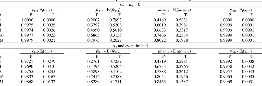
Table 3 presents the decomposition of the forecast error variance of the levels of c; f e; daw and y into the components that can be attributed to the three permanent shocks combined and to the transitory shock. I identify the transitory shock as orthogonal to the three permanent shocks. The top panel reports the variance decomposition if statistically insigni…cant adjust- ment coe¢ cient estimates are set to zero as recommended by Gonzalo and Ng (2001). The bottom panel displays the variance decomposition if all ad- justment coe¢ cients are set to their estimated values.

The transitory shock should have the strongest e¤ect on the forecast error variance of both asset wealth components because their adjustment coe¢ cient estimates are statistically signi…cant. This implies that both of the variables participate in the correction of a temporary deviation from the common trends among c; f e; daw and y and hence should be primarily driven by the transitory shock. The variance decompositions mirror exactly this reasoning. Note also that the impact of the transitory shock on the variance of foreign equity is stronger than on domestic asset wealth which is in line with the magnitude of the error correction coe¢ cient estimates.

The foreign equity adjustment coe¢ cient is substantially larger than that

of domestic asset wealth, i.e. the transitory shock has to have a stronger impact on foreign equity than on domestic asset wealth. Consumption and labour income do not participate in the error correction. Their adjustment coe¢ cients are statistically indistinguishable from zero, which means that both variables should be predominantly driven by the permanent shocks.

Variance decompositions for consumption and labour income support this reasoning. Almost all of the variation of consumption and labour income can be attributed to the three permanent shocks at any time horizon.

3 Forecasting power of the cointegration resid- ual

The estimated adjustment coe¢ cients and the variance decompositions imply that the cointegration residual should serve as a predictor of changes of U.S.

households´ foreign equity holdings.

I perform long-horizon regressions with the cointegration residual as sole regressor to assess this point. The long- horizon regressions take the following general form

X

h=1

y

= +

x

+ "

(16) where x is the cointegration residual, y the natural logarithm of the regres- sand, denotes a constant and " the error terms at the respective time horizon t + h.

I focus on in-sample regressions to provide evidence for predictability throughout this paper since out-of sample regressions do not necessarily pro- vide superior, more robust, results in favour or against predictability (Inoue and Kilian, 2004). But before describing the evidence it may be useful to provide some intuition of what should be re‡ected in the regression out- comes. A temporarily high consumption-wealth ratio is associated with the expectation of high future returns on aggregate wealth. The positive sign of the foreign equity error correction coe¢ cient estimate suggests that we should expect positive regressor estimates in forecast regressions of market value changes of foreign equity holdings on the cointegration residual because

6

Lettau and Ludvigson (2004) show that the cointegration residual neither predicts

consumption nor labour income growth.

a temporarily high U.S. consumption-wealth ratio is associated with a high market value of foreign equity holdings.

High expected returns on foreign stock markets induce households to increase their foreign equity investment and thus the market value of their foreign equity holdings. Hence, positive regressor estimates in forecast regres- sions of excess returns on foreign stock indexes on the cointegration residual would be the consequence. However, this reasoning does not necessarily have to apply to all foreign stock markets. So, I cannot preclude negative estimates in regressions of national stock returns on the cointegration residual.

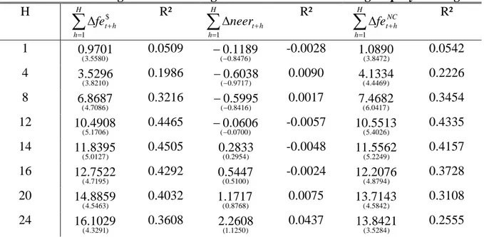
The left column of table 4 presents estimates from the regression of changes of U.S. households´ foreign equity holdings, f e

, on b

x

with Newey-West corrected t-statistics in parenthesis. The forecast horizon, h, is in quarters. All regressor coe¢ cient estimates are statistically signi…cant.

The R

statistic peaks at 14 quarters and displays that the cointegration residual explains 45 percent of the variation of foreign equity holdings in U.S. wealth.

However, foreign equity holdings are denominated in current U.S. dol- lars. Predictability then means that changes of the quantity of foreign eq- uity, changes of the price of foreign equity in local currency or changes of the nominal U.S exchange rate vis-à-vis the rest of the world or an arbitrary combination are responsible for a correction of the cointegration error and hence predictable. In order to shed light on this issue, I construct a foreign equity investment weighted e¤ective exchange rate of the U.S. dollar relative to the countries the U.S. hold equity of. I focus on countries in which the U.S. invest at least one percent of their foreign equity investment.

The 17 countries used in this analysis represent about 80% of U.S. foreign equity investment. Data on foreign equity investment is from the IMF´s coordi- nated portfolio survey 2001. I use the share of U.S. equity investment into a particular country from total U.S. foreign equity investment as a weight to construct the e¤ective exchange rate. I assume these weights, derived from 2001 data, to be constant over the sample period from …rst quarter 1957 to third quarter 2003. This assumption certainly biases the e¤ective exchange rate towards the foreign equity investment pattern of the U.S. in

7

I omit equity investment in o¤shore markets as Bermuda or Cayman Islands and con-

centrate on Australia, Canada, Finland, France, Germany, Hong Kong, Ireland, Italy,

Japan, Korea, Mexico, Netherlands, Sweden, Singapore, Spain, Switzerland and the

United Kingdom.

recent years. However, foreign equity ‡ows have grown substantially since the last twenty years (Hau and Rey (2004)), such that shares of U.S. foreign equity investment in recent years appropriately display where and to what extent the U.S. invest in foreign equity. The weights described above should thus be su¢ cient to approximate the true foreign equity investment weighted e¤ective U.S. dollar exchange rate.

If exchange rate changes of the US-dollar relative to the countries the U.S.

hold equity of are responsible for temporary ‡uctuations of foreign equity holdings, then the cointegration residual will forecast changes of the equity investment weighted exchange rate. Moreover, I investigate if changes of for- eign equity holdings denominated in a weighted basket of national currencies are predictable. I employ the equity investment weighted exchange rate to obtain foreign equity holdings in such a compound currency. Predictability of changes of these holdings either re‡ects variation of equity prices in lo- cal currency or changes of the quantity of foreign equity holdings or both.

However, these e¤ects cannot be distinguished in this exercise.

The middle column of table 4 provides evidence that changes of the e¤ec- tive exchange rate, neer are not predicted by the cointegration residual for the time period from …rst quarter 1957 to third quarter 2003. None of the regressor coe¢ cients is statistically distinguishable from zero. This result is corroborated by not reported regressions of bilateral exchange rate changes on the cointegration residual.

The non-predictability of exchange rate changes leaves the impression that b

x

predicts changes of foreign equity holdings in local currency, f e

. The right column of table 4 presents the regression results. All regressor coe¢ cients are statistically distinguishable from zero. The peak of predictability is reached after 12 quarters explaining 43 percent of foreign equity holdings variation if they are expressed in a weighted basket of national currencies. The evidence of predictability is as strong as in the case of foreign equity holdings denominated in U.S. dollar.

The forecast regressions reported in table 4 reveal that the cointegration residual displays information about market value changes of U.S. households´

foreign equity holdings. The non-predictability of exchange rate changes conveys the notion that the correction of the cointegration error through foreign equity holdings is caused by the expectation of time-varying returns on foreign stock markets and subsequent portfolio rebalancing. Exchange

8

Results are available upon request.

rate changes play a negligible role in the error correction mechanism.

At this stage, however, it is not clear whether households react to the perception of exchange rate adjusted expected returns or to returns in local currency. In order to assess this point I examine if b

x

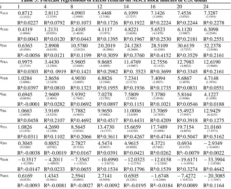
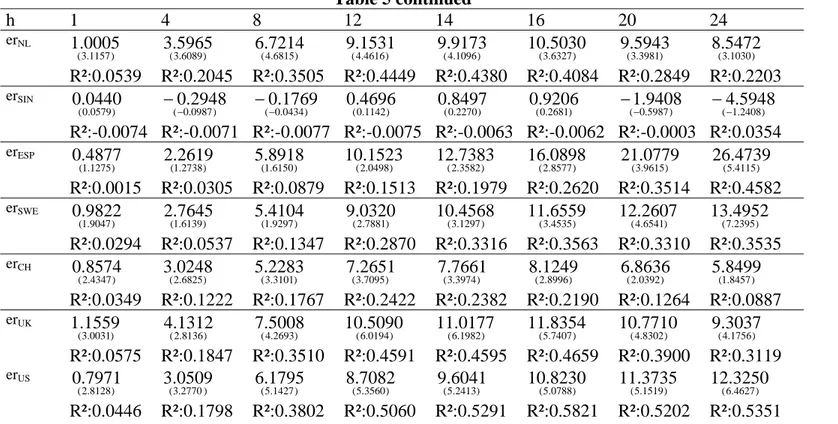
predicts excess returns on Morgan Stanley Capital International (MSCI) stock indexes for the countries employed to calculate the e¤ective exchange rate. The MSCI indexes o¤er the advantage that the methodology of index construction is the same for all country indexes and hence allows for direct comparison. Fur- thermore, MSCI publishes index values with underlying market capitalisation denominated in U.S. dollar and local currency.

Table 5 reports estimates from long-horizon regressions when excess re- turns on MSCI indexes with underlying market capitalisation in U.S. dollars are regressed on the cointegration residual. Newey-West corrected t-statistics appear in parenthesis. The forecast horizon, h, is in quarters. The sample covers the period from fourth quarter 1969 to second quarter 2004, except for Finland, Ireland, Korea and Mexico. The sample period for Finland spans the period from …rst quarter 1982 to second quarter 2004, the sample period for Ireland, Korea and Mexico covers the …rst quarter 1988 to second quarter 2004. Excess returns are de…ned as simple return on a country index less the three-month U.S. treasury bill rate at the beginning of period, re‡ecting the U.S. investor´s opportunity cost of investing in a foreign stock market.

The regression results of table 5 mirror that the cointegration residual

predicts excess returns with underlying market capitalisation in U.S. dollars

best at 8 to 24 quarter frequency. With the exception of Japanese, Mexican

and Singaporean stock index returns, which are not predictable at any time

horizon, 14 MSCI stock index returns in U.S. dollars are predictable. The

predictive power of the cointegration residual di¤ers widely across countries,

at most 11,5 percent of the variation of excess returns on the Hong Kong

MSCI index is explained by b

x

compared to 51,6 percent for Italy. A

notable outlier is Korea, which displays forecastability at long horizons, 12

to 24 quarters, but the regressor coe¢ cient is negative, in contrast to the

economic intution given at the beginning of the section. However, an expla-

nation for this …nding is straightforward. During the short sample period

for which data on the Korean MSCI stock index is available, Korea experi-

enced a severe currency crisis which had signi…cant negative impact on the

Korean stock market while the U.S. enjoyed the stock market boom of the

late 1990s right at the time of the Korean currency crisis which leads to the

negative estimates. A high U.S. consumption-wealth ratio is thus associated with negative returns on the Korean stock market.

Noteworthy as well is the predictive power of b

x

for excess returns on the German MSCI index. It explains about 20% of the German stock index return variation. The U.S. consumption-wealth ratio re‡ects ‡uctuations of the German stock market, whereas the German consumption-wealth ratio displays ‡uctuations of the German unemplyoment rate and other business cycle variables (Hamburg et al. (2005)).

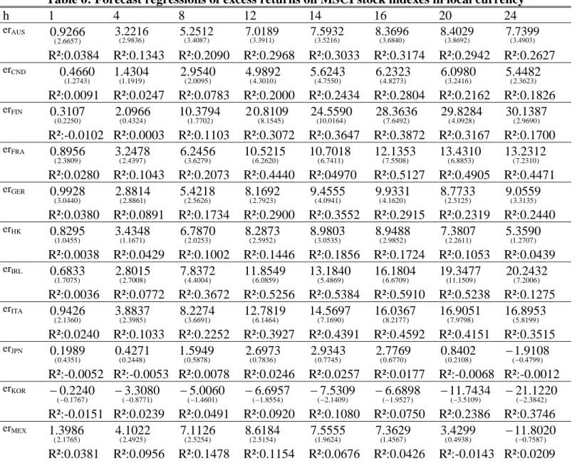
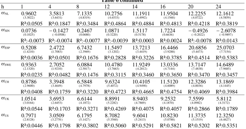
Table 6 reports estimates from forecast regressions of excess returns on MSCI stock indexes with underlying market capitalisation in local currency on the cointegration residual. The overall picture that emerges is that excess returns in national currency are at least equally predictable as returns de- nominated in U.S dollars. The predictive power of the cointegration residual for excess returns in local currency leaves the impression that temporary ‡uc- tuations of foreign equity holdings are induced by the expectation of expected returns in local currencies rather than exchange rate adjusted returns.

4 Robustness check and implications for stock market comovement

The long-horizon regressions in the previous section suggest that short-run

‡uctuations of the U.S. consumption-wealth ratio explain close to one half of the variation in long-horizon returns on some of the foreign country indexes.

This result suggests that b

x

re‡ects an important common, cyclical com- ponent in international stock markets which could be interpreted as risk fac- tor common to international stock market returns. But how reliable are the results from the forecast regressions? Does variation in the U.S. consumption- wealth ratio really capture short-run movements of international stock mar- kets? Or are the high R

statistics obtained in the long-horizon regressions spurious?

Figures 1 (a) to (h) plot actual realisations of 16-quarter returns on coun-

try indexes for which the forecast regressions provided R

statistics of around

0.4 or higher together with the …tted values of the cointegration residual for

that time horizon. Note that the return series are denominated in local

currency. The countries in question are France, Ireland, Italy, Netherlands,

Spain, Switzerland, United Kingdom and the United States. I consider re-

turns from beginning of the 1970s to present for all countries except Ireland.

The …gures show that the high R

statistics for long-horizon returns on the country indexes under consideration indeed re‡ect the explanatory power of variation in the U.S. consumption-wealth ratio for short-term movements of international stock markets. The relationship between actual long-horizon returns and …tted values of the cointegration residual is far from being spuri- ous. Quite in contrast, the …tted short-run ‡uctuations of the ratio between consumption and aggregate wealth in the U.S. provide a good description of the variation in returns on international stock markets. Hence, the …gures support the view that the U.S. consumption-wealth ratio echoes a common, transitory component in international stock markets.

Thus the cointegration residual seems to represent a risk factor common to international stock markets which explains a considerable fraction of the variation in long-horizon returns. As this risk factor is common to stock markets and mirrored in the U.S. consumption-wealth ratio, we could ob- tain information about the degree of covariation between international stock markets from

var(r) =

var(cay) + cov(") (17)

where r is the vector of long-horizon returns, cay represents the cointegra- tion residual, i.e. the common risk factor and the vector of loadings on the risk factor which are the regressor coe¢ cients from the long-horizon regres- sions at a particular time horizon. The vector of error terms is represented

by ": If the common risk factor re‡ected in cay explains all of the variation

in and covariation between long-horizon returns, then the covariance matrix of the error terms contains only zeros.

Hence, the error term covariance matrix divided by the covariance matrix

of the long-horizon returns shows how much of the actual return variation

and how much of the covariation between stock markets is not explained by

the common risk factor, cay. The diagonal elements of that matrix display

the fraction of variation in long-horizon returns that is not explained by

cay, whereas the o¤-diagonal elements mirror how much of the covariation

between the return series is not explained by the common factor. In order to

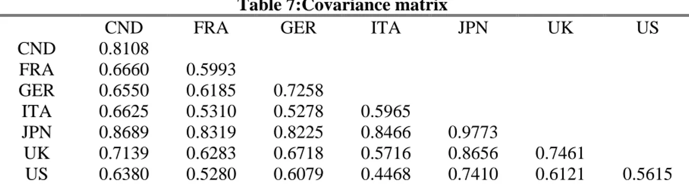
serve space I focus on the 16-quarter, local curency returns on stock indexes of

the G7 economies. Table 7 presents the results. The values on the diagonal

re‡ect that the common factor explains between 20 to 45 percent of the

variation of long-horizon returns on the G7 stock indexes except Japan. As

suggested by the forecast regressions almost all of the variation in returns on

the Japanese stock market remain unexplained by cay. Hence the forecast regressions are corroborated.

The o¤-diagonal elements display how much of the comovement between the G7 stock markets is not explained by the common component. Not surprisingly very little of the Japanese stock market´s covariation with the other G7 economies is captured by the common risk factor. However, cay explains between one third and more than a half of the covariation between 16-quarter local currency returns on the remaining G7 stock markets. The unexplained covariation could be caused by a common permanent component in international stock markets or due to country-speci…c e¤ects as suggested by Richards (1995). However, this …nding highlights the importance of the common, cyclical stock market component in explaining the comovement of international stock markets at business cycle frequency.

5 Conclusions

Comovement of international stock markets on the one hand and macro- economic explanations of stock return predictability on the other hand are individually well documented. However, a robust link between international stock markets at business cycle frequency has not been established yet.

By employing a simple manipulation of the theoretical framework pro- posed by Lettau and Ludvigson (2001,2004), I demonstrate that temporary

‡uctuations in the market value of U.S. households´ foreign equity holdings are induced by time-varying returns on foreign stock markets. Time variation of returns displays variation in risk premia. Hence, short-run ‡uctuations of the U.S. consumption-wealth ratio predict excess returns, a proxy for risk pre- mia, on international stock markets. This …nding suggests the existence of an important transitory component common to international stock markets that explains a considerable fraction of short-term variation in international stock returns.

Furthermore, between one third and one half of the covariation between long-horizon returns on stock markets of the G7 economies can be explained by the so far undiscovered common, temporary component which underlines its importance for the comovement of international stock markets.

Additionally, U.S. households seem to rebalance their equity portfolios

in response to the perception of local currency rather than exchange rate

adjusted returns as the cointegration residual explains local currency returns

at least equally well as returns denominated in U.S. dollar. Moreover, ex- change rate changes do not seem to cause cyclical variation in the market value of U.S. households´ foreign equity holdings which is mirrored in the non-predictablity of exchange rate changes by the cointegration residual.

Acknowledgements

This paper constitutes the …rst part of my Ph.D. thesis at the University of Dortmund. I substantially bene…ted from numerous discussions with my supervisor Mathias Ho¤mann. Moreover, I am especially grateful for com- ments and remarks by James Nason as well as participants in the 5th IWH Macroeconometric Workshop, the 9th International Conference on Macro- economic Analysis and International Finance, the 12th Global Finance Con- ference and the 37th Annual Conference of the Money, Macro and Finance Research Group.

Research in this paper is funded by the Deutsche Forschungsgemeinschaft

through SFB 475 (Reduction of complexity in multivariate data structures),

project B6: International Allocation of Risk.

References

[1] Beveridge, Stephen and Charles R. Nelson (1981), "A new approach to decomposition of economic time series into permanent and transitory components with particular attention to the measurement of the busi- ness cycle", Journal of Monetary Economics, vol. 7, pp. 151-174.

[2] Blinder, Alan S. and Angus Deaton (1985), "The Time Series Consump- tion Revisited", Brookings Papers on Economic Activity, 2, pp. 465-511.

[3] Brooks, Robert and Marco Del Negro (2005), "Firm-Level Evidence on International Stock Market Comovement", forthcoming Review of Finance.

[4] Campbell, John Y. (1996), "Understanding Risk and Return", The Jour- nal of Political Economy, vol. 104, no. 2, pp. 298-345.

[5] Campbell, John Y. and John H. Cochrane (1999), "By Force of Habit:

A Consumption-Based Explanation of Aggregate Stock Market Behav- iour", The Journal of Political Economy, 107, pp.205-251.

[6] Campbell, John Y. and Gregory Mankiw (1989), "Consumption, income and interest rates: Reinterpreting the time series evidence", in: Blan- chard, Olivier; Fischer, Stanley (eds.) NBER Macroeconomics Annual, MIT Press Cambridge MA.

[7] Campbell, John Y. and Robert J. Shiller (1988), "The Dividend Price Ratio and Expectation of Future Dividends and Discount Factors", Re- view of Financial Studies, 1, pp. 195-227.

[8] Cochrane, John H., (2005), "Financial Markets and the Real Economy", NBER working paper 11193.

[9] Constantinides, George M. and Darrell Du¢ e (1996), "Asset Pricing with Heterogeneous Consumers", The Journal of Political Economy, vol.

104, issue 2 (April), pp.219-240.

[10] Engle, Robert F. and Clive W.J. Granger (1987), "Co-Integration And

Error Correction: Representation, Estimation and Testing", Economet-

rica, vol. 55, no. 2, pp. 251-276.

[11] Fernandez-Corugedo, Emilio, Simon Price and Andrew Blake (2003),

"The dynamics of consumer´s expenditure: the UK consumption ECM redux", Bank of England working paper 204.

[12] Fisher, Lance A. and Graham M. Voss (2004), "Consumption. Wealth and Expected stock returns in Australia", The Economic Record, vol.

80, no. 251, pp. 359-372.

[13] Gonzalo, Jesus and Serena Ng (2001), "A Systematic Framework for Analyzing the Dynamic E¤ects of Permanent and Transitory Shocks", Journal of Economic Dynamics and Control, 25(10), pp. 1527-1546.

[14] Hamburg, Britta, Mathias Ho¤mann and Joachim Keller (2005), "Con- sumption, Wealth and Business Cycles: Why is Germany di¤erent?", Deutsche Bundesbank discussion paper 16/2005.

[15] Hau, Herbert and Hélène Rey (2004), "Can Portfolio Rebalancing Ex- plain the Dynamics of Equity Returns, Equity Flows, and Exchange Rates?", American Economic Review P&P, 94, no. 2, pp.126-133.

[16] Heaton, John and Deborah Lucas (2000a), "Portfolio Choice in the Pres- ence of Background Risk", The Economic Journal, 110, pp.1-26.

[17] Heaton, John and Deborah Lucas (2000b), "Portfolio Choice and As- set Prices: The Importance of Entrepreneurial Risk", The Journal of Finance, vol. 55, no. 3, pp. 1163-1198.

[18] Ho¤mann, Mathias (2001), "The relative Dynamics of Investment and the Current Account in the G7-Economies", The Economic Journal, vol.

111, no. 471, pp.148-168.

[19] Ho¤mann, Mathias (2005), "Proprietary Income and the Predictability of Stock Returns", mimeo, University of Dortmund

[20] Ho¤mann, Mathias and Ronald Mc Donald (2003), "A Re-Examination of the link between Real Exchange Rates and Real Interest Rate Di¤er- entials", CESifo working paper no. 894.

[21] Inoue, Atsushi and Lutz Kilian (2004), "In-sample or out-of-sample tests

of predictability: which one should we use?", Econometric Reviews,

23(4), pp. 1-32

[22] Johansen, Sören (1995), "Likelihood-based inference in cointegrated vek- tor autoregressive models", Oxford University Press.

[23] Kasa, Kenneth (1992), "Common stochastic trends in international stock markets", Journal of Monetary Economics 29, pp. 95-124.

[24] Lettau, Martin and Sydney Ludvigson (2001), "Consumption, Aggre- gate Wealth and Expected Stock Returns", The Journal of Finance, 56, no. 3, pp. 815-849.

[25] Lettau, Martin and Sydney Ludvigson (2004), "Understanding Trend and Cycle in Asset Values: Reevaluating the Wealth E¤ect on Con- sumption", American Economic Review, vol. 94, no. 1, pp.276-299.

[26] Richards, Anthony J. (1995), "Comovements in national stock market returns: Evidence of predictability, but not cointegration", Journal of Monetary Economics, 36, pp. 631-654.

[27] Rudd, Jeremy and Karl Whelan (2002), "A Note on the Cointegration of Consumption, Income and Wealth", FEDS working paper No. 2002-53.

[28] Stock, James H. (1987), "Asymptotic Properties Of Least Squares Es- timators Of Cointegrating Vectors", Econometrica, vol. 55, no. 5, pp.

1035-1056.

[29] Stock, James H. and Mark W. Watson (1988), "Testing for Common Trends", Journal of the American Statistical Association, 83, pp. 1093- 1107.

[30] Stock, James H. and Mark W. Watson (1993), "A Simple Estimator of Cointegrating Vectors In Higher Order Integrated Systems", Economet- rica, vol. 61, no. 4, pp. 783-820.

[31] Tan, Alvin and Graham M. Voss (2003), "Consumption and Wealth in Australia", The Economic Record, vol. 79, no. 244, pp. 39-56.

[32] Tesar, Linda L. and Ingrid M. Werner (1995), "Home Bias and High

Turnover", Journal of International Money and Finance, vol. 14, no. 4,

pp. 467-492.

Data appendix

U.S. household stock market wealth includes directly held equity shares at market value and indirectly held equity shares in the form of bank personal trusts and estates holdings, life insurance companies´ hold- ings, private pension fund holdings, state and local government as well as federal government fund holdings and household´s mutual fund hold- ings as published in the supplemental table B.100e in the Z1 Flow of Funds Accounts of the Federal Reserve Board. However, this table is not available at quarterly frequency such that quarterly stock market wealth has to be constructed from Flow of Funds tables L.213 and L.214.

– Table L.213 lists direct holdings of corporate equity at market value distinguished by the respective holders. According to the de…nition above, direct equity holdings of the household sector (line 6), bank personal trusts and estates (line 11), life insurance companies (line 12), private pension funds (line 14), state and local government (line 15) as well as federal government corporate equity holdings (line 16) are included in stock market wealth. I calculate the amount of equities held by U.S. households through mutual fund holdings with help of table L.214.

– Table L.214 lists direct holdings of mutual fund shares at market value distinguished by the respective holders. In order to calculate the amount of equities held by U.S. households through mutual fund holdings, I take the fraction of e.g. direct household mutual fund shares holdings at market value and multiply it with the di- rect holding of corporate equities by mutual funds (L.213, line 17).

I apply this procedure to all components of stock market wealth listed above which hold mutual fund shares and hence indirectly corporate equity.

The share of foreign equity in household net worth is derived from

Flow of Funds table L.213 which provides details about equity issues

and holdings at market value. Corporate equity issues at market value

include holdings of foreign issues by U.S. residents inclusive American

Depositary Receipts. I assume that the share of this rest-of-the-world

equity holdings in total corporate equity holdings is the same as the

share of rest-of-the-world equity holdings in U.S. households´ corporate equity holdings because U.S. households either directly or indirectly hold about 90% of total corporate equity issues.

U.S. household domestic asset wealth is the di¤erence between house- hold net worth, Z1 ‡ow of funds table B.100, line 42, and U.S. foreign equity holdings de…ned above.

U.S. consumption is consumption expenditure on non-durable goods and services excluding shoes and clothing published by the Bureau of Economic Analysis in NIPA table 2.3.5. Data on total personal consumption expenditure is also taken from NIPA table 2.3.5.

Data on U.S. labour income is freely available from the Bureau of Eco- nomic Analysis in NIPA table 2.1. I follow Lettau and Ludvigson who de…ne labour income as wages and salaries disbursements (line 3) + employer contribution for employee pension and insurance funds (line 7) + personal current transfer receipts (line 16) - contributions for gov- ernment social insurance (line 24) - labour taxes. Labour taxes are de…ned as {wages and salaries disbursements / [wages and salaries dis- bursements + proprietors´ income with inventory valuation and capital consumption adjustment (line 9) + rental income of persons with cap- ital consumption adjustment (line 12) + personal interest income (line 14) + personal dividend income (line 15)]} times [personal taxes (line 25) + personal current transfer payments (line 30)].

The CPI of total personal consumption expenditure in chain-weighted (2000 = 100) seasonally adjusted U.S. dollars published by the Bu- reau of Economic Analysis in NIPA table 1.1.4. is used to obtain real variables.

The Bureau of Economic Analysis publishes population …gures in NIPA table 2.1, which are used to obtain per capita …gures.

The nominal e¤ective foreign equity investment exchange rate is a geo-

metrically weighted average of the nominal U.S. dollar spot exchange

rates with Australia, Canada, Finland, France, Germany, Hong Kong,

Ireland, Italy, Japan, Korea, Mexico, Netherlands, Sweden, Singapore,

Spain, Switzerland and United Kingdom. The weights are derived from

the IMF´s Coordinated Portfolio Survey of Equity Investment and re-

‡ect how large the share of U.S. equity investment in the respective country was in 2001. I assume that this share is constant over the sam- ple period from …rst quarter 1957 to third quarter 2003. The source of bilateral U.S. dollar spot exchange rates is the IMF´s International Financial Statistic January 2004. I use the dollar-euro exchange rate for all EMU member countries under consideration since 1999.

I de…ne excess returns on MSCI indizes as return at the end of quarter

minus the risk-free rate at the beginning of quarter, re‡ecting the op-

portunity cost of a U.S. investor investing in foreign equity. Returns are

the natural logarithm of the respective index value at the end of time

t+1 minus the natural logarithm of the index value at the end of time

t. The risk-free rate is the 3-month-U.S. treasury bill. Since I regard

logarithmic approximations of net returns (continuously compounded

returns), the h-period return is the sum of the one period returns over

h periods.

Tables

Table 1: Johansen Cointegration Test

Critical Values Trace Test Statistic Trace

10% 5% 1%

r=0 44.4929 47.8545 54.6815 44.1243 r=1 27.0669 29.7961 35.4628 19.0531 r=2 13.4294 15.4943 19.9349 3.6106

r=3 2.7055 3.8415 6.6349 0.0150

Critical Values L-Max Test Statistic L-Max

10% 5% 1%

r=0 25.1236 27.5858 32.7172 25.0711 r=1 18.8928 21.1314 25.8650 15.4426 r=2 12.2971 14.2639 18.5200 3.5955

r=3 2.7055 3.8415 6.6349 0.0150

AIC SIC

l=1 -22.0350 -21.7791 l=2 -21.9342 -21.4224

Notes: The variables under consideration are non-durables and services consumption expenditure excluding expenditures on clothing and shoes, foreign equity holdings, domestic asset wealth and labour income. All variables are measured at quarterly frequency. The sample starts second quarter 1952 and ends second quarter 2004. All variables are in natural logarithms, real, p.c. in 2000 chain weighted U.S. dollars.

The Johansen test is performed under the assumption of an unrestricted constant but no time trend in the data.

The Trace test tests the null hypothesis of r cointegrating relations against the alternative of p, the number of

variables in the tested system, cointegrating relations. The L-Max test tests the null of r cointegrating relations

against the alternative of r+1. AIC is the Akaike information criterion, SIC the Schwartz information criterion.

Table 2: VECM estimates

∆c

∆fe

∆daw

∆y

∆c

) 2462 . 3 (

. 2412 0

) 9277 . 1 (

. 2414 3

) 2248 . 2 (

. 7594 0

) 2615 . 3 (

. 5450 0

∆fe

) 0310 . 1 (

0 . 0032

−

) 1311 . 1 (

. 0799

0

0

.

0174

−

) 5113 . 1 (

. 0106 0

∆daw

) 2726 . 0 (

0 . 0048

−

) 5910 . 0 (

0 . 2366

−

) 0942 . 1 (

. 0889 0

) 5099 . 1 (

0 . 0601

−

∆y

) 5886 . 2 (

. 0922

0 0

.

7503

) 5606 . 1 (

. 2555

0

0

.

1192

−

´

ˆ x

β

0

.

0113

−

) 3255 . 4 (

. 2974 1

) 6996 . 3 (

. 2254 0

) 1445 . 0 (

0 . 0043

−

Notes: This table reports VECM estimates for the cointegrated VAR consisting of non-durable consumption and services consumption expenditure excluding clothing and shoes, c, foreign equity, fe, domestic asset wealth, daw, and labour income, y, for the sample period from second quarter 1952 to second quarter 2004. ˆ ´

−

x

β is

the cointegration residual. T-statistics are in parenthesis.

Table 3: Forecast error variance decompositions of the levels of the four cointegrated variables α

= α

= 0

c

-E

(c

) fe

- E

(fe

) daw

- E

(daw

) y

- E

(y

)

h P T P T P T P T

1 1.0000 0.0000 0.2007 0.7993 0.4169 0.5831 1.0000 0.0000

4 0.9975 0.0025 0.3792 0.6208 0.6019 0.3981 0.9999 0.0001

8 0.9974 0.0026 0.4990 0.5010 0.6683 0.3317 0.9999 0.0001

16 0.9977 0.0023 0.6865 0.3135 0.7466 0.2534 0.9999 0.0001

24 0.9979 0.0021 0.7973 0.2027 0.8022 0.1978 0.9999 0.0001

α

and α

estimated

c

-E

(c

) fe

- E

(fe

) daw

- E

(daw

) y

- E

(y

)

h P T P T P T P T

1 0.9721 0.0279 0.2761 0.7239 0.4719 0.5281 0.9992 0.0008

4 0.9690 0.0310 0.4796 0.5204 0.6735 0.3265 0.9958 0.0042

8 0.9755 0.0245 0.5898 0.4102 0.7388 0.2612 0.9957 0.0043

16 0.9833 0.0167 0.7412 0.2588 0.8044 0.1956 0.9965 0.0035

24 0.9868 0.0132 0.8289 0.1711 0.8463 0.1537 0.9969 0.0031

Notes: This table reports the forecast error variance share of the level of the cointegrating variables, consumption, c, foreign equity, fe, domestic asset wealth, daw and labour

income, y, that can be attributed to the combined three permanent shocks (columns “P”) and the single transitory shock (columns “T”). The forecast horizon h is in quarters.

Table 4: Forecast regressions of changes of U.S. households´ foreign equity holdings

H ∑

=

∆

H

h

h

fe

$

R²

∑

∆

h

neer

R² ∑

=

∆

H

h

NC h

fe

R² 1

) 5580 . 3 (

. 9701

0 0.0509

) 8476 . 0 (

0 . 1189

−

-0.0028

) 8472 . 3 (

. 0890

1 0.0542

4

) 8210 . 3 (

. 5296

3 0.1986

) 9717 . 0 (

0 . 6038

−

0.0090

) 4469 . 4 (

. 1334

4 0.2226

8

) 7086 . 4 (

. 8687

6 0.3216

) 8416 . 0 (

0 . 5995

−

0.0017

) 0417 . 6 (

. 4682

7 0.3454

12

) 1706 . 5 (

. 4908

10 0.4465

) 0700 . 0 (

0 . 0606

−

-0.0057

) 4026 . 5 (

. 5513

10 0.4335

14

) 0127 . 5 (

. 8395

11 0.4505

) 2954 . 0 (

. 2833

0 -0.0048

) 2249 . 5 (

. 5562

11 0.4157

16

) 7195 . 4 (

. 7522

12 0.4292

) 5100 . 0 (

. 5447

0 -0.0024

) 8794 . 4 (

. 2076

12 0.3728

20

) 5463 . 4 (

. 8859

14 0.4032

) 8768 . 0 (

. 1717

1 0.0075

) 5842 . 4 (

. 7143

13 0.3108

24

) 3291 . 4 (

. 1029

16 0.3608

) 1250 . 1 (

. 2608

2 0.0437

) 5284 . 3 (

. 8421

13 0.2555

Notes: This table reports OLS estimates from long-horizon regressions using the cointegration residual as sole regressor. The forecast horizon h is in quarters. The sample spans the period from second quarter 1952 to second quarter 2004 for ∆fe

and first quarter 1957 to third quarter 2003 for ∆neer and ∆fe

. R² reports values of the adjusted R². Newey-West corrected t-statistics are displayed in parenthesis.

The first column provides estimates from the regression of changes of U.S. households´ foreign equity holdings in U.S. dollar terms, ∆fe

on the cointegration residual.

The middle column gives estimates from the regression of changes of the foreign equity investment weighted nominal effective U.S. dollar exchange rate, ∆neer, on the cointegration residual.

The right column presents estimates from the regression of changes of U.S. households´ foreign equity holdings

in terms of a weighted basket of national currencies, ∆fe

on the cointegration residual.