Tuning PSO Parameters Through Sensitivity Analysis

Tuning PSO Parameters Through Sensitivity Analysis

Thomas Beielstein

, Konstantinos E. Parsopoulos

, Michael N. Vrahatis

1

Department of Computer Science XI, University of Dortmund, D–44221 Dortmund, Germany.

thomas.beielstein@LS11.cs.uni-dortmund.de

2

Department of Mathematics, Artificial Intelligence Research Center (UPAIRC), University of Patras, GR–26110 Patras, Greece

{kostasp, vrahatis}@math.upatras.gr

Abstract- In this paper, a first analysis of the Particle Swarm Optimization (PSO) method’s parameters, using Design of Experiments (DOE) techniques, is performed, and important settings as well as interactions among the parameters, are investigated (screening).

1 INTRODUCTION

Computer experiments and simulations play an important role in scientific research, since many real–world processes are so complex that physical experimentation is either time con- suming or expensive. Simulation models often need high–

dimensional inputs and they are computationally expensive.

Thus, the simulation practitioner is interested in the develop- ment of simulation models, that enable him to perform the simulation with the minimum amount of simulation runs. To achieve this goal, design of experiments (DOE) methods have been developed and successfully applied in the last decades.

The DOE techniques can be applied to optimization algo- rithms, considering the run of an algorithm as an experiment, gaining insightful conclusions into the behavior of the algo- rithm and the interaction and significance of its parameters.

In this paper, the parameters of the Particle Swarm Optimiza- tion method (PSO) are investigated using DOE techniques.

The rest of the paper is organized as follows: the PSO method and the DOE techniques are briefly described in Sec. 2 and 3, respectively. An experimental design (DESIGN I) is chosen and experiments (simulation runs) are performed.

This design is discussed in detail in Sec. 4, and an improved design (DESIGN II) is developed. The analysis results in rec- ommendations for the parameter setting of PSO on a special test function, that are statistically validated.

2 PARTICLE SWARM OPTIMIZATION

The term “Swarm Intelligence”, is used to describe algo- rithms and distributed problem solvers inspired by the col- lective behavior of insect colonies and other animal societies [BDT99, KE01]. Under this prism, PSO is a Swarm Intel- ligence method for solving optimization problems. Its pre- cursor was a simulator of social behavior, that was used to visualize the movement of a birds’ flock. Several versions

of the simulation model were developed, incorporating con- cepts such as nearest–neighbor velocity matching and accel- eration by distance [ESD96, KE95]. When it was realized that the simulation could be used as a population–based opti- mizer, several parameters were omitted, through a trial and error process, resulting in the first simple version of PSO [EK95, ESD96].

Suppose that the search space is

–dimensional, then the

–th individual, which is called

, of the popula- tion, which is called

, can be represented by a

– dimensional vector,

=(x

i1

;x

i2

;:::;x

iD )

>

. The velocity (position change) of this particle, can be represented by an- other

–dimensional vector

=(v

i1

;v

i2

;:::;v

iD )

>

. The best previously visited position of the

–th particle is denoted as

=(p

i1

;p

i2

;:::;p

iD )

>

. Defining

as the index of the best particle in the swarm (i.e. the

–th particle is the best), and let the superscripts denote the iteration number, then the swarm is manipulated according to the following two equa- tions [ESD96]:

v n+1

id

= v n

id +cr

n

1 (p

n

id x

n

id )+cr

n

2 (p

n

g d x

n

id );

(1)

x n+1

id

= x n

id +v

n+1

id

;

(2)

where

;

, and

is the size of the swarm;

is a positive constant, called acceleration con- stant;

,

are random numbers, uniformly distributed in

[0;1]

; and

, determines the iteration number.

However, in the first version of PSO, there was no actual control mechanism for the velocity. This could result in inef- ficient behavior of the algorithm, especially in the neighbor- hood of the global minimum. In a second version of PSO, this shortcoming was addressed by incorporating new parameters, called inertia weight and constriction factor. This version is described by the equations [ES98, SE98b, SE98a]:

v n+1

id

= (w v n

id +c

1 r

n

1 (p

n

id x

n

id )+

+c

2 r

n

2 (p

n

g d x

n

id )

;

(3)

x n+1

id

= x

n

id +v

n+1

id

;

(4)

where

is called inertia weight;

,

are two positive con- stants, called cognitive and social parameter respectively; and

is a constriction factor, which is used to limit velocity.

The role of the inertia weight

, in Eq. (3), is consid- ered critical for the PSO’s convergence behavior. The iner- tia weight is employed to control the impact of the previous history of velocities on the current one. Accordingly, the pa- rameter

regulates the trade–off between the global (wide–

ranging) and local (nearby) exploration abilities of the swarm.

A large inertia weight facilitates global exploration (search- ing new areas), while a small one tends to facilitate local ex- ploration, i.e. fine–tuning the current search area. A suitable value for the inertia weight

usually provides balance be- tween global and local exploration abilities and consequently results in a reduction of the number of iterations required to locate the optimum solution. Initially, the inertia weight was constant. However, experimental results indicated that it is better to initially set the inertia to a large value, in order to promote global exploration of the search space, and gradu- ally decrease it to get more refined solutions [SE98b, SE98a].

Thus, an initial value around

and a gradual decline to- wards

can be considered as a good choice for

.

Proper fine–tuning of the parameters

and

, in Eq. (3), may result in faster convergence of the algorithm, and alle- viation of the local minima. An extended study of the ac- celeration parameter in the first version of PSO, is given in [Ken98]. As default values,

=c

2

=2

were proposed, but experimental results indicate that

=c

2

=0 :5

might pro- vide even better results. Recent work reports that it might be even better to choose a larger cognitive parameter,

, than a social parameter,

, but with

+c

2

64

[CD01].

The parameters

and

are used to maintain the diversity of the population, and they are uniformly distributed in the range

. The constriction factor

controls on the magni- tude of the velocities, in a way similar to the

parameter, used in the first versions of PSO. In some cases, using both

and

may result in faster convergence rates. In all exper- iments in this paper, the PSO method described in Eqs. 3 and 4, with

was used.

Although PSO is an evolutionary technique, it differs from other evolutionary algorithm (EA) techniques. Three main operators are usually involved in EA techniques. The re- combination, the mutation and the selection operator. PSO does not have a direct recombination operator. However, the stochastic acceleration of a particle towards its previ- ous best position, as well as towards the best particle of the swarm (or towards the best in its neighborhood in the local version), resembles the recombination procedure in EA [ES98, Rec94, Sch75, Sch95]. In PSO the information exchange takes place only among the particle’s own expe- rience and the experience of the best particle in the swarm, instead of being carried from fitness dependent selected “par- ents” to descendants as in GA’s. Moreover, PSO’s directional position updating operation resembles mutation of GA, with a kind of memory built in. This mutation–like procedure is multi-directional both in PSO and GA, and it includes con- trol of the mutation’s severity, utilizing factors such as the

V

max

and

.

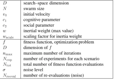
Symbol Parameter

D

search–space dimension

N

swarm size

v

0

initial velocity

c

1

cognitive parameter

c

2

social parameter

w

inertial weight (max value)

w

scale

scaling factor for inertia weight

f

fitness function, optimization problem

D

dimension of

n

max

maximum number of iterations

N

exp

number of experiments for each scenario

N

tot

total number of fitness function evaluations

noise level

N

reeval

number of re-evaluations (noise) Table 1: DOE parameter.

Var Factor I: Level II: Level

N A f600;900;1200g f10;30

;50g

w B f0:6;0:9;1:2g f0:3;0:6

;0:9g

w

scale

C f0:0;0:25;0:5g f0:0;0:25;0:5

g

c

1

D f0:5;1:0;2:0g f0:5;1:0

;2:0g

c

2

E f0:5;1:0;2:0g f1:75;2:25

;2:75g

Table 2: DESIGN I and DESIGN II.

PSO belongs to the class of EAs, that does not use the

“survival of the fittest” concept. It does not utilize a direct selection function. Thus, particles with lower fitness can sur- vive during the optimization and potentially visit any point of the search space [ES98].

3 EXPERIMENTAL DESIGN

Experimental design provides an excellent way of deciding which simulation runs should be performed so that the de- sired information can be obtained with the least amount of experiments [BHH78, BD87, Kle87, KVG92, Kle99, LK00].

The input parameters and structural assumptions, that define a simulation model are called factors, the output value(s) are called response(s). The different values of parameters are called levels. An experimental design is a set of factor level combinations. As mentioned in Sec. 2, fine–tuning of PSO parameters is an important task. The role of the inertia weight

w

, the relationship between the cognitive and the social pa- rameters

and

or the determination of the swarm size are important to ensure convergence of the PSO algorithm. Ap- plying the DOE model assumptions to PSO algorithms, we can define the parameter vector (cp. Tab. 1):

p=(N;v

0

;c

1

;c

2

;w ;w

scale )

T

(5)

and the design vector:

d=(f;D ;n

max

;N

exp

;N

tot

;N

reeval

; ) T

:

(6)

−80

−60

−40

−20 0

A0

−80

−60

−40

−20 0

A1

−80

−60

−40

−20 0

A2

−80

−60

−40

−20 0

B0

−80

−60

−40

−20 0

B1

−80

−60

−40

−20 0

B2

−80

−60

−40

−20 0

C0

−80

−60

−40

−20 0

C1

−80

−60

−40

−20 0

C2

−80

−60

−40

−20 0

D0

−80

−60

−40

−20 0

D1

−80

−60

−40

−20 0

D2

−80

−60

−40

−20 0

E0

−80

−60

−40

−20 0

E1

−80

−60

−40

−20 0

E2

−80

−60

−40

−20 0

total

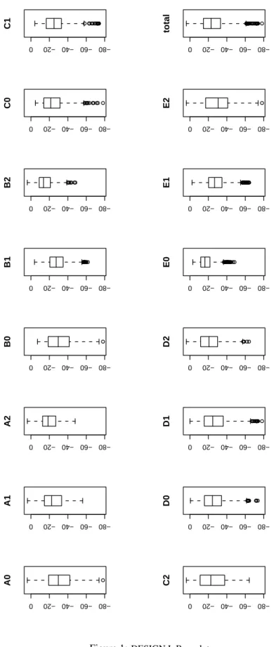
Figure 1: DESIGN I. Box-plot

−40−35−30−25−20−15

A

mean of Y

600 900 1200

B 1.2 0.9 0.6

−32−28−24−20

A

mean of Y

600 900 1200

C 0.5 0 0.25

−30−25−20

A

mean of Y

600 900 1200

D 2 0.5 1

−35−30−25−20−15

A

mean of Y

600 900 1200

E 0.5 2 1

−35−30−25−20−15−10

B

mean of Y

0.6 0.9 1.2

C 0.5 0 0.25

−30−25−20−15−10

B

mean of Y

0.6 0.9 1.2

D 2 1 0.5

−45−35−25−15

B

mean of Y

0.6 0.9 1.2

E 0.5 2 1

−28−26−24−22−20

C

mean of Y

0 0.25 0.5

D 2 0.5 1

−35−30−25−20−15

C

mean of Y

0 0.25 0.5

E 2 0.5 1

−30−25−20

D

mean of Y

0.5 1 2

E 0.5 2 1

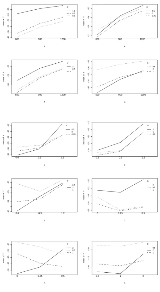
Figure 2: DESIGN I. Interaction plot

In the next section, we will apply DOE methods to improve the behavior of the PSO algorithm for a given optimization configuration. This task can be interpreted as the determina- tion of optimal values of

for a given problem design

or as an analysis of a regression meta-model [KVG92].

4 SENSITIVITY ANALYSIS APPLIED TO PSO

Starting point for the first experiments is the minimization of the sphere function

P

D

i=1 x

2

i

;

were

. Al- though the number of simulation runs required increases ge- ometrically with

for a

factorial design as

is increased, we chose a

full factorial design for didactical purposes.

3

l

factorial designs clarifies the geometrical interpretation of the results. Neglecting higher order interactions, fractional factorial designs reduce the required amount of simulation runs drastically [BHH78]. Efficiency and effectiveness of de- signs are discussed in [Kle87, KVG92]. The corresponding factor levels are shown in Tab. 2. To apply analysis of vari- ance (ANOVA) techniques, we have to verify classical as- sumptions, e.g. the ‘normality of errors’ [DS98].

Examination of the fit reveals, that the main effects and some first order interactions are significant, but that it is nec- essary to use a response transformation

. After check- ing the fitted regression model, we investigate the effects and their interactions

.

Box-plots provide an excellent visualization of the effects of a change of one factor level. For a factor

,

denotes the low,

the medium, and

the highest value. Regard- ing the swarm size

in DESIGN I, we obtain:

:

,

A1

:

, and

:

. Thus we can conclude from the first three plots in Fig. 1, that the swarm size should be set to the low

level.

outperforms the other

factor level set- tings, but

and

should be set to their medium level values (

=0 :25

resp.

=1 :0

), whereas

should be set to its maximum value

.

Fig. 2 shows the interactions between two factors. The first figure reveals, that factor

performs best at its low level

600

– no matter how we set factor

. Obviously performs

best, if we choose its low level

, too. But we have to be careful, since the ANOVA shows that the interaction

is not significant.

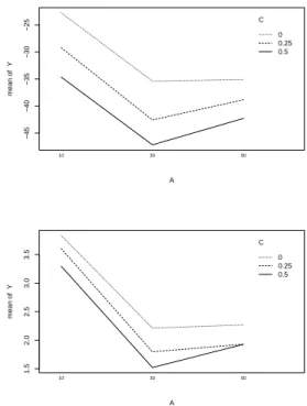
Results from the analysis of DESIGN I lead to an im- proved DESIGN II. The following investigations were based on DESIGN II (corresponding settings marked with an aster- isk in Tab. 2). We investigated the transferability of the results to other designs by modifying two parameters of the design vector

(cp. Eq. 6): Dimension

and noise

.

Increasing the search-space dimension does not change the behavior of the PSO significantly: Fig.3 reveals the behavior of the PSO for

and

(instead of

in Fig. 2). As a first result, we can conclude: The general

1R, a language for data analysis and graphics was used to perform the ANOVA and to generate the graphics in this paper [IG96].

behavior of the PSO on the sphere model does not change, if the search space dimension is modified. Adding normal dis- tributed noise to the fitness function value does change the behavior of the PSO and requires different strategy parame- ters to obtain convergence.

−45−40−35−30−25

A

mean of Y

10 30 50

C 0 0.25 0.5

1.52.02.53.03.5

A

mean of Y

10 30 50

C 0 0.25 0.5

Figure 3: DESIGN II. Varying the search-space dimension:

24

(above) and

(below).

5 Summary and Outlook

In this paper, a first analysis of the PSO method’s parameters, using DOE techniques, was introduced, and important param- eter settings and interactions were extracted (screening).

Extension to other fitness functions and real–world prob- lems, are needed to verify the insightful results obtained in this paper. Currently, experiments on the simplified elevator simulator (S-ring) [MAB

01], are performed to improve the efficiency of the design (fractional designs). A comparison of PSO and other stochastic search methods, especially EAs, will be given in future work.

Acknowledgments

This work is a product of the Collaborative Research Cen- ter ‘Computational Intelligence’ (531), at the University of Dortmund and was supported by the Deutsche Forschungs- gemeinschaft (DFG).

2These results will not be discussed here, but will be published in a forth- coming paper.

Bibliography

[BD87] G. E. P. Box and N. R. Draper. Experimental Model Building and Response Surfaces. Wiley, 1987.

[BDT99] E. Bonabeau, M. Dorigo, and G. Theraulaz.

Swarm Intelligence: From Natural to Artificial Systems. Oxford University Press, New York, 1999.

[BHH78] G. E. P. Box, W. Hunter, and J. S. Hunter. Statis- tics for experimenters. Wiley series in probabilty and mathematical statistics: Applied probability and statistics. Wiley, 1978.

[CD01] A. Carlisle and G. Dozier. An Off-The-Shelf PSO. In Proceedings of the Particle Swarm Op- timization Workshop, pages 1–6, 2001.

[DS98] N. R. Draper and H. Smith. Applied regression analysis. Wiley series in probability and statis- tics. Wiley, New York, 3 edition, 1998.

[EK95] R.C. Eberhart and J. Kennedy. A New Opti- mizer Using Particle Swarm Theory. In Proceed- ings Sixth Symposium on Micro Machine and Human Science, pages 39–43, Piscataway, NJ, 1995. IEEE Service Center.

[ES98] R.C. Eberhart and Y. Shi. Comparison Between Genetic Algorithms and Particle Swarm Opti- mization. In V.W. Porto, N. Saravanan, D. Waa- gen, and A.E. Eiben, editors, Evolutionary Pro- gramming VII, pages 611–616. Springer, 1998.

[ESD96] R.C. Eberhart, P. Simpson, and R. Dobbins.

Computational Intelligence PC Tools. Academic Press, 1996.

[IG96] R. Ihaka and R. Gentleman. R: A language for data analysis and graphics. Journal of Compu- tational and Graphical Statistics , 5(3):299–314, 1996.

[KE95] J. Kennedy and R.C. Eberhart. Particle Swarm Optimization. In Proceedings IEEE Interna- tional Conference on Neural Networks, pages 1942–1948, Piscataway, NJ, 1995. IEEE Service Center.

[KE01] J. Kennedy and R.C. Eberhart. Swarm Intelli- gence. Academic Press, London, 2001.

[Ken98] J. Kennedy. The Behavior of Particles. In V.W. Porto, N. Saravanan, D. Waagen, and A.E.

Eiben, editors, Evolutionary Programming VII, pages 581–590. Springer, 1998.

[Kle87] J. Kleijnen. Statistical Tools for Simulation Practitioners. Marcel Dekker, New York, 1987.

[Kle99] J. Kleijnen. Validation of models: Statistical techniques and data availability. In P.A. Farring- ton, H.B. Nembhard, D.T. Sturrock, and G.W.

Evans, editors, Proceedings of the 1999 Winter Simulation Conference, pages 647–654, 1999.

[KVG92] J. Kleijnen and W. Van Groenendaal. Simulation - A Statistical Perspective. Wiley, Chichester, 1992.

[LK00] A. M. Law and W. Kelton. Simulation Modelling and Analysis. McGraw-Hill Series in Industrial Egineering and Management Science. McGraw- Hill, New York, 3 edition, 2000.

[MAB

01] Sandor Markon, Dirk V. Arnold, Thomas Bäck, Thomas Beielstein, and Hans-Georg Beyer.

Thresholding – a selection operator for noisy ES. In Proc. Conference on Evolutionary Com- putation (CEC 2001) , Seoul, Korea, May 27–30, 2001.

[Rec94] I. Rechenberg. Evolution Strategy. In J.M. Zu- rada, R.J. Marks II, and C. Robinson, editors, Computational Intelligence: Imitating Life, Pis- cataway, NJ, 1994. IEEE Press.

[Sch75] H.-P. Schwefel. Evolutionsstrategie und nu- merische Optimierung. Dr.-Ing. Thesis, Techni- cal University of Berlin, Department of Process Engineering, 1975.

[Sch95] H.-P. Schwefel. Evolution and Optimum Seek- ing. Wiley, New York, 1995.

[SE98a] Y. Shi and R.C. Eberhart. A Modified Parti- cle Swarm Optimizer. In Proceedings of the IEEE Conference on Evolutionary Computation, pages 69–73, Piscataway, NJ, 1998. IEEE Press.

[SE98b] Y. Shi and R.C. Eberhart. Parameter Selection in Particle Swarm Optimization. In V.W. Porto, N. Saravanan, D. Waagen, and A.E. Eiben, edi- tors, Evolutionary Programming VII, pages 591–

600. Springer, 1998.