arXiv:hep-ph/0102257v1 21 Feb 2001

arXiv:hep-ph/0102257v1 21 Feb 2001

UCSD/PTH 00-25 MPI-PhT/2001-04 hep-ph/0102257

The Running Coulomb Potential and Lamb Shift in QCD

Andre H. Hoang^∗

Max-Planck-Institut f¨ur Physik (Werner-Heisenberg-Institut)

F¨ohringer Ring 6, 80805 M¨unchen, Germany

Aneesh V. Manohar^†, Iain W. Stewart^‡

Department of Physics, University of California at San Diego, 9500 Gilman Drive, La Jolla, CA 92093, USA

Abstract

The QCDβ-function and the anomalous dimensions for the Coulomb po- tential and the static potential first differ at three loop order. We evaluate the three loop ultrasoft anomalous dimension for the Coulomb potential and give the complete three loop running. Using this result, we calculate the lead- ing logarithmic Lamb shift for a heavy quark-antiquark bound state, which includes all contributions to the binding energies of the formm α⁴_s(αslnαs)^k, k≥0.

Typeset using REVTEX

∗ahoang@mppmu.mpg.de

†amanohar@ucsd.edu

‡iain@schwinger.ucsd.edu

I. INTRODUCTION

In this paper, we construct the three-loop anomalous dimension for the Coulomb po- tential in non-relativistic QCD (NRQCD) [1,2]. The formalism we use was developed in Refs. [3–6] and will be referred to as vNRQCD, an effective theory for heavy non-relativistic quark-antiquark pairs. Part of our computation is related to the running of the static po- tential [7], however effects associated with motion of the quarks do play an important role.

Our final result for the Coulomb potential differs from the static potential at terms beyond those with a single logarithm (i.e. starting at four loops). Combining our Coulomb potential running with previous results for the running of the 1/mand 1/m² potentials [4,6] allows us to compute the next-to-next-to-leading logarithmic (NNLL) corrections in the perturbative energy of a heavy QQ¯ bound state, which includes the sum of terms m α⁴_s(αslnαs)^k,k ≥0, where m is the heavy quark pole mass. This contribution is the QCD analog of the QED α⁵lnαLamb shift computed by Bethe. In QED, the seriesm α⁴(αlnα)^kterminates after the k = 1 term [8]. In QCD, there is an infinite series due to the running QCD coupling as well as the presence of non-trivial anomalous dimensions for other QCD operators. The results presented here also contribute to the NNLL prediction for the cross section for e⁺e⁻ → t¯t near threshold [9]. Implications forb¯b sum rules will be addressed in a future publication.

The expansion parameter of the effective theory is the quark velocity v. A quark has a momentum of order mv and an energy of order mv². We assume that m is large enough thatmv² ≫ΛQCD and a perturbative description of the bound state as a Coulombic system is valid. For a Coulombic bound state, αs is of order v and contributions suppressed by bothv and αs are of the same order. It is useful to distinguish between powers of αs and v when carrying out the matching and when evolving couplings and operators in the effective theory, and to only take v ∼αs for the power counting of bound state matrix elements. In the effective theory, the quark-antiquark potentials appear as four-quark operators [2]. A potential of the formα^r_s/|k|^s is of orderα_s^rv^1−s, where kis the fermion momentum transfer.

With this power counting the time-ordered product of av^a and v^b potential is of order v^a+b. Up to next-to-next-to-leading order (NNLO) the heavy quark potential has contributions

V ∼

αs

v

+

α²_s v

+

α³_s

v +α²_sv⁰+αsv

+. . . . (1)

The order αs/v ∼1 term in Eq. (1) is the Coulomb potential generated at tree-level. The next-to-leading order (NLO) term is the one-loop correction to the Coulomb potential. The

NNLO terms are the two-loop correction to the Coulomb potential, the one-loop value for the 1/(m|k|) potential, and the tree-level contribution to the order |k|⁰/m² potential. Writing theQQ¯ energy asE = 2m+∆E, the terms in Eq. (1) generate contributions of the following order in the binding energy:

∆E ∼^hmα²_sⁱ+^hmα³_sⁱ+^hmα⁴_sⁱ+. . . . (2) In Eqs. (1) and (2) the expansion has been performed at the scale µ = m so the cou- pling constants are αs=αs(m). A typical perturbative expansion contains logarithms of µ divided by the various physical scales in the bound state. If the logarithms are large, fixed order perturbation theory breaks down, and one finds a large residual µ dependence. One can minimize the logarithms by setting µ to a value appropriate to the dynamics of the non-relativistic system. This is accomplished by summing large logarithms using the renor- malization group, and using renormalization group improved perturbation theory. For QQ¯ bound states, the large logarithms are logarithms of v ∼αs, and can be summed using the velocity renormalization group (VRG) [3]. For the binding energy this gives the expansion

∆E = ∆E^LL+ ∆E^{N LL}+ ∆E^{N N LL}+. . . , (3)

∼

m

∞

X

k=0

α^k+2_s (lnαs)^k

+

m

∞

X

k=0

α^k+3_s (lnαs)^k

+

m

∞

X

k=0

α^k+4_s (lnαs)^k

+. . . , where the terms are the leading log (LL), next-to-leading log (NLL), and next-to-next-to- leading log (NNLL) results respectively.

In the VRG, one uses a subtraction velocityνthat is evolved from 1 tov. This simultane- ously lowers the momentum cutoff scaleµS =mν fromm tomv and the energy cutoff scale µU =mν² frommtomv². The VRG properly accounts for the coupling between energy and momentum caused by the equations of motion for the non-relativistic quarks. QED provides a highly non-trivial check of the VRG method. In Ref. [8] it was used to correctly repro- duce terms in the subleading series of logarithms, including the α³ln²α corrections to the ortho and para-positronium decay rates, the α⁷ln²α hyperfine splittings for Hydrogen and positronium, and the α⁸ln³α Lamb shift for Hydrogen. The difference between the VRG, which involves the evolution of the momentum and the energy scale in a single step, and a conventional two stage renormalization group treatment, m → mv → mv², was examined in Ref. [10].

In section II we review the definition of potentials for non-static heavy quarks in the effective theory. In section III we compare these potentials with the Wilson loop definition

which is appropriate for static quarks. In section IV we rederive the leading-logarithmic (LL) and next-to-leading-logarithmic (NLL) results for theQQ¯ binding energy using the effective theory and discuss the two-loop matching for the Coulomb potential using the results in Refs. [11,12]. We also discuss some subtleties in the correspondence between diagrams in the static theory and soft diagrams in the effective theory. In section V we compute the three-loop anomalous dimension for the Wilson coefficient of the Coulomb potential.

Results for the NNLL energy are given in section VI, followed by conclusions in section VII.

In Appendix A we give some technical details on the structure of divergences in the effective theory, and in Appendix B we list some functions that appear in the energy at NNLL order.

II. THE VNRQCD POTENTIALS

The effective theory vNRQCD has soft gluons with coupling constant αS(ν), ultrasoft gluons with coupling constant αU(ν), as well as quark-antiquark potentials. The potential is the momentum dependent coefficient of a four-fermion operator:

L=−^X

p,p^′

V (p,p^′) ^hψp^′†

ψpχ−p^′†

χ−p

i, (4) where spin and color indices are suppressed. The coefficient V (p,p^′) has an expansion in powers of v, V = V₍₋₁₎+V₍₀₎ +V₍₁₎+. . ., where V₍₋₁₎ = Vc is the Coulomb potential. For equal mass fermions

Vc = (T^A⊗T¯^A)V_c^(T)

k² + (1⊗1)V_c⁽¹⁾ k² , V(0) = (T^A⊗T¯^A)π²V_k^(T)

m|k| + (1⊗1)π²V_k⁽¹⁾ m|k| , V₍₁₎ = (T^A⊗T¯^A)





V₂^(T)

m² + V_s^(T)S²

m² +V_r^(T)(p²+p^′2)

2m²k² − iV_Λ^(T)S·(p^′×p)

m²k² +V_t^(T)T(k) m²





+(1⊗1)





V₂⁽¹⁾

m² +V_s⁽¹⁾ m² S²



, (5)

wherek=p^′−p,S= (σ₁+σ₂)/2,T(k) = (δ^ij−3kⁱk^j/k²)σⁱ

1σ^j

2. The Wilson coefficients, V^(T,1) depend on the subtraction velocity ν. In Eq. (5) the color decomposition V = (T^A⊗ T¯^A)V^(T)+ (1⊗1)V⁽¹⁾ has been used and the potential in the color singlet channel isV^(s) = V⁽¹⁾−CFV^(T). (The Casimirs of the adjoint and fundamental representations are denoted by

CA and CF, respectively.) At LL order the running of the coefficients V_2,s,r^(1,T) was computed in Ref. [4] and V_Λ,t^(1,T) in Ref. [4,13], while the NLL order running of V_k^(1,T) was computed in Ref. [6]. In this work we compute the running of V_c^(s) at NNLL order. This allows the computation of the QQ¯ energy spectrum at NNLL order.

In vNRQCD additional potential-like effects are generated by loops with soft gluons, for which the Feynman rules can be found in Refs. [3,5]. Matrix elements of soft gluon diagrams contribute to the energy beginning at NLO. In contrast, matrix elements with ultrasoft gluons start at N³LO. The renormalization group improved energies are obtained by computing the anomalous dimensions for these soft interactions and the four fermion operators in Eq. (5).

III. THE STATIC POTENTIAL VERSUS THE COULOMB POTENTIAL

Parts of our analysis are related to the study of the static limit of QCD which describes heavy quarks in the m → ∞ limit. We therefore briefly review the pertinent results which have been derived in this framework.

In position space the static QCD potential is defined as the expectation value of the Wilson loop operator,

Vstat(r) = lim

T→∞

1 T ln

TrPexp−ig

I

CAµdx^µ

, (6)

where C is a rectangle of width T and fixed height r. This potential is independent of the mass m of the quarks and depends only on r. In QCD perturbation theory the static potential is known at two-loop order [11,12] . These calculations use static fermion sources with propagators which are identical to those in Heavy Quark Effective Theory [14]. The exponentiation of the static potential [15,16] guarantees that one can avoid dealing with graphs which have pinch singularities in momentum space. The analysis of Refs. [15,16]

also gives a prescription for the color weight factors for different graphs based on the c-web theorem.

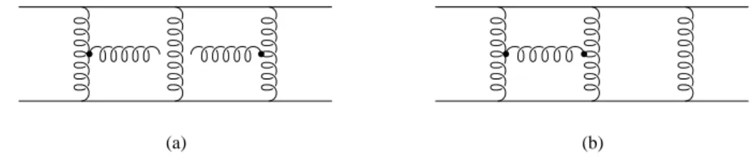
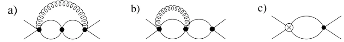
In Ref. [17], Appelquist, Dine and Muzinich (ADM) pointed out that at three loops the static potential in Eq. (6) has infrared (IR) divergences from graphs of the form in Fig. 1a,b.

In the color singlet channel Fig. 1a has color factor CFC_A²(CA −2CF) while Fig. 1b is proportional to C_F²C_A². Taking into account the exponentiation of Vstat using the c-web theorem, the color singlet contribution to Vstat from Fig. 1(a,b) is simply Fig. 1a with the

(a) (b)

FIG. 1. Graphs contributing to the three-loop IR divergence of the QCD static potential.

color factor replaced by C_A³CF, and is IR divergent. ADM showed that this IR divergence could be avoided by summing a class of diagrams—those of Fig. 1 with the addition of an arbitrary number of gluon rungs. Summing over these diagrams regulates the IR divergence by building up Coulombic states for the static quark sources. The summation gives a factor exp[V^(s)(r)−V^(o)(r)]Tfor the propagation of the intermediate color-octetQQ¯ pair, where V^(s)(r) and V^(o)(r) are the color-singlet and color-octet potentials. The exponential factor suppresses long-time propagation of the intermediate color-octet state, and regulates the IR divergence by introducing an IR cutoff scale of order [V^(s)(r)−V^(o)(r)]∼αs/r.

In Ref. [18] the ADM divergence in the static potential was studied by Brambilla et al. using the effective theory pNRQCD [2]. They made the important observation that along with potential contributions, the definition in Eq. (6) contains contributions from ultrasoft gluons, and the latter are responsible for the ADM IR divergence. They showed that the ADM IR divergence in QCD matches with an IR divergence of a pNRQCD graph that describes the selfenergy of a quark-antiquark system due to an ultrasoft gluon with momenta q^µ ∼ αs/r. Therefore, the static potential in pNRQCD can be defined as a matching coefficient of a four fermion operator, as in Eq. (4), in an infrared safe manner.

We will refer to this potential as the soft-static potential. The ultrasoft pNRQCD graph also has an ultraviolet divergence. Brambilla et al. computed the coefficient of this divergence and extracted a new ln(µ) contribution to the soft-static potential. In Ref. [7] the three-loop anomalous dimension was computed for the soft-static potential in this framework. In the color singlet channel for scales µ∼αs(r)/r their solution reads

Vstat(µ, r) = V_stat^(2loops)(r)− 1 4πr

"

2πCFC_A³ 3β0

α³_s(r) ln

αs(r) αs(µ)

#

, (7)

where the first term is the two loop static potential derived in Refs. [11,12].

For large but finite m the effective theory for QQ¯ bound states has an expansion in v. The quark potential in this case differs from that in the static case, and in general one cannot obtain the static theory by taking the m → ∞ limit. To illustrate this consider as

FIG. 2. Loop with an insertion of the 1/(m|k) and 1/k² potentials.

an example the loop graph involving the iteration of a 1/(m|k|) and a Coulomb potential as shown in Fig. 2. In the effective theory for non-static fermions, the fermion propagators give a factor proportional tom. The final result for the graph is independent ofmand is the same order inv as the Coulomb potential. On the other hand, if we first take the static limit m→ ∞, then 1/(m|k|)→0, and there is no such graph. This example illustrates the general result that the static theory is not obtained as them→ ∞(orv →0) limit of the non-static effective theory. Loop integrals can produce factors of m or 1/v, and thereby cause mixing between operators which are of different orders¹ in v. Furthermore, the energy and the momentum transfer in Coulombic states are coupled by the quark equations of motion. We will see that for this reason the anomalous dimension of the static and Coulomb potentials differ at three loops. The three-loop matching for the static and Coulomb potentials can also differ.

IV. THE COULOMB POTENTIAL AT ONE AND TWO LOOPS

In this work dimensional regularization and the MS scheme will be used. The MS QCD running coupling constant will be denoted by α_s(µ), and is determined by the solution of the renormalization group equation

µdα_s(µ)

dµ =β(α_s(µ))

=−2β0

α_s²(µ) 4π −2β1

α_s³(µ) (4π)² −2β2

α_s⁴(µ)

(4π)³ +. . . . (8) In a mass-independent subtraction scheme β0 andβ1 are scheme-independent. The notation α_s^[n](µ) will be used to indicate the solution of Eq. (8) with coefficients up to βn−1 (i.e. n loop order) kept in the β-function.

In the VRG, the soft and ultrasoft subtraction scales µS and µU are given by µS =mν and µU = mν². We define the soft and ultrasoft anomalous dimensions γS and γU as the

1However, we stress that if powers of αs are also counted as powers of v, then operators which are higher order inv never mix into lower order operators.

derivatives with respect to lnµS and lnµU, respectively. The derivative with respect to lnν gives the total anomalous dimension, γ = γS + 2γU. vNRQCD has three independent but related coupling constants that are relevant for our calculation: the soft gluon coupling αS(ν), the ultrasoft gluon coupling αU(ν), and the coefficient of the Coulomb potential Vc(ν). The tree-level matching conditions at (µ=m⇔ν = 1) are

αS(1) =αU(1) =α_s(m), V_c^(T)(1) = 4πα_s(m), V_c⁽¹⁾(1) = 0, (9) and the solutions of the one-loop renormalization group equations for the coupling constants in the effective theory are [19,3]

αS(ν) =α_s^[1](mν), αU(ν) =α_s^[1](mν²),

V_c^(T)(ν) = 4πα_s^[1](mν), V_c⁽¹⁾(ν) = 0. (10) In deriving the above equations, it has been assumed that any light fermions have masses much smaller than mv², so that there are no mass thresholds in the renormalization group evolution. If there is a mass threshold larger than mv² and widely separated from mv and m, then it is possible to also include such effects in the effective theory, see Ref. [3].

At leading order the Hamiltonian for the color singlet QQ¯ system is H₀ = p²

m +V_c^(s)(ν)

k² . (11)

To minimize large logarithms in higher order matrix elements we run ν to the bound state velocity vb, which we define as the solution of the equation

vb = ac(ν =vb)

n = CF α_s^[1](mvb)

n , (12)

where for convenience we have defined

ac(ν) =− V_c^(s)(ν)

4π , (13)

andnis the principal quantum number. The LL binding energy is then simply the eigenvalue of the Schr¨odinger equation, H0|ψn,li = ∆E|ψn,li with the LL solution for the Coulomb potential, V_c^(s)(ν) =−CFV_c^(T)(ν) from Eq. (10). Thus,

∆E^LL =− m

4n² [ac(ν)]² (14a)

=− m

4n² C_F^{2 h}α_s^[1](mvb)ⁱ² =−mv_b²

4 , (14b)

where in the second line we have evaluated the energy at the low scale ν =vb. Higher order corrections to the energy are all evaluated as perturbative matrix elements with the leading order wavefunctions, |ψn,li.

Consider how the results in Eq. (10) are extended to higher orders. The graphs for the renormalization of the ultrasoft gluon self coupling have the same rules as for QCD, and those for the renormalization of the lowest order soft gluon vertex have the same rules as for HQET. Since the momenta of soft and ultrasoft gluons are cleanly separated there is no mixing of scales, so the anomalous dimension for αS is independent of αU and vica-versa.

Thus, one expects that in the MS scheme αS(ν) = α_s(mν) and αU(ν) = α_s(mν²) to all orders.

However, the coefficient of the Coulomb potential can differ from 4πα_s(mν) at higher orders. At one-loop, the only orderα²_s/v graph in the effective theory is the soft diagram [5]²

= −iµ^2ǫ_Sα_S²(ν)

k² (T^A⊗T¯^A)

β0

ǫ +β0lnµ²_S k²

+a1

, (15)

where β0 = 11/3CA−4TFnℓ/3 and a1 = 31CA/9−20TFnℓ/9 in the MS scheme, and nℓ is the number of light soft quarks. The divergence in Eq. (15) is canceled by a counterterm for V_c^(T), causing it to run with anomalous dimension −2β0α²_S(ν). The remaining terms in the soft graph are identical to the one-loop soft-static potential calculation and also reproduce the set of α²_s/k² terms in full QCD with dimensional regularization parameter µ. The one- loop matching correction to V_c^(T,1)(1) is the difference between the full and effective theory diagrams and therefore vanishes at the matching scale µ=µS =m.

A correspondence between the soft-static potential calculation and soft order 1/v dia- grams is expected to persist at higher orders in αs as well. The Feynman rules for the soft vertices are almost identical to the HQET rules used for soft-static potential calculations.

There are a few notable differences. In the effective theory it is not necessary to use the exponentiation theorem [15,16] to eliminate diagrams with pinch singularities of the form

Z

dq⁰ 1

(q0 +iǫ)(−q0 +iǫ). (16)

These are automatically removed in the construction of the tree level soft vertices because the 1/q₀ factors in the soft Feynman rules do not contain iǫ’s, and in evaluating diagrams

2Note that the soft loop includes soft gluons, soft light quarks, as well as soft ghosts.

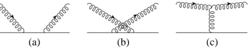
(a) (b) (c)

FIG. 3. Compton scattering graphs that contribute to the soft vertex.

(a) (b)

FIG. 4. Examples of vertices involving soft gluons.

these poles are ignored. For example [3], from matching the full theory Compton scattering graphs in Fig. 3 one obtains the soft vertex in Fig. 4a which is proportional to [T^A, T^B]/q0, where terms proportional to {T^A, T^B} have canceled. In the soft-static calculations this cancellation instead takes place at the level of the box and crossed box graphs, and is guaranteed by exponentiation. For the soft-static potential it is known that at higher orders there are contributions from the iπδ(q0) terms that originate from the iǫ’s. It was exactly this type of contribution that was missed in the two-loop calculation by Peter [11], and was correctly identified by Schr¨oder [12]. In the effective theory these delta function contributions belong to the potential regime [6], and soft-static graphs with this type of contribution are reproduced by operators such as the one shown in Fig. 4b, where a soft gluon scatters from a potential. Matching induces these operators to account for the difference between the full and effective theory graphs for Compton scattering off two quarks. Thus, the treatment of iǫ’s does affect the correspondence between soft-static and soft graphs. The total contribution of the graphs in the static theory with k^µ∼mv gluons is reproduced in the effective theory by graphs with soft gluons.

A real difference between the soft-static and effective theory calculations is the way in which counterterms are implemented. The soft-static potential is defined by local HQET-like Feynman rules and all UV divergent contributions from soft gluons are absorbed into vertex, field, and coupling renormalization. The renormalization of the four point function is taken care of by the renormalization of the two and three point functions. Renormalization of the vNRQCD diagrams is quite different because potential gluons are not treated as degrees of freedom. The effective theory has graphs with soft gluons and in addition the four-quark

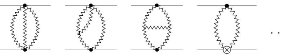
V_c V₍₁₎ V_c V_c V_c V₍₁₎ V_c V_c V_c ^Vc V₍₀₎

FIG. 5. Order α³_s/v diagrams with potential iterations. The × denotes an insertion of the p⁴/8m³ relativistic correction to the kinetic term.

. . .

FIG. 6. Examples of order α³_s/v diagrams with soft vertices. The vertex with a cross denotes an insertion of a one-loop counterterm.

Coulomb potential operator. The overall divergence in soft graphs, such as the one in Eq. (15), are absorbed byVc, while subdivergences are taken care of by counterterms for the soft vertices and lower order Vc counterterms. The sum of unrenormalized soft-static and purely soft diagrams in the effective theory agree. So if these were the only considerations, then the description of these effects would be basically a matter of convenience. However, divergences associated with ultrasoft gluons can only be absorbed into Vc, so at the level that these gluons contribute in the effective theory it is necessary to adopt the four quark operator description from the start (i.e. just below the scale m).

To calculate the NLL energy we also need the two-loop anomalous dimension for Vc, which is obtained from the renormalization of orderα_s³/v diagrams. At this order there are effective theory graphs with iterations of potentials, shown in Fig. 5, and soft effective theory diagrams, as in Fig. 6. Graphs with ultrasoft gluons do not contribute at this order. The potential diagrams are finite in the ultraviolet and reproduce the Coulombic singularities in perturbative QCD. The contributions from the soft diagrams can be determined from the soft-static potential calculations. For the color singlet channel, the UV divergences in the soft-static two-loop diagrams were calculated in Ref. [20] and the constant terms in Refs. [11,12]. The sum of unrenormalized soft diagrams has the form

iα³_S(ν) k²

CF

4π

β₀²

ǫ² + β1+2β0a1

ǫ + 2β₀²

ǫ lnµ²_S k²

+β₀²ln²µ²_S k²

+(β1+2β0a1) lnµ²_S k²

+a^(a)₂

. (17) The effective theory counterterm graphs give

−iα_S³(ν) k²

CF

4π

2β₀²

ǫ² +2β₀²

ǫ lnµ²_S k²

+2a1β0

ǫ +a^(b)₂

. (18)

Taking the sum of Eqs. (17) and (18) we find that up to two-loops the counterterm for the color singlet Coulomb potential has the form

Zc = 1− αS(ν)β0

4πǫ + α²_S(ν) (4π)²

β₀² ǫ² −β1

ǫ

, (19)

where β1 = 34C_A²/3−4CFTFnℓ−20CATFnℓ/3. The α²_s/ǫ divergence is proportional to β1, so the two-loop anomalous dimension forV_c^(s) is determined by the two-loop MS β-function, and the NLL coefficient of the singlet Coulomb potential is V_c^(s)(ν) = 4πα_s^[2](mν).

The energy at NLL order involves including the NLL coefficient for the Coulomb poten- tial, V_c^(s)(ν) in Eq. (14a), and calculating the matrix element of the one-loop order 1/v soft diagram between Coulombic states [ac(ν)≡ −V_c^(s)(ν)/4π]

i

* +

=−CF α_S²(ν)

* 1 k²

a1+β0lnµ²_S k²

+

(20)

=−m CFα_S²(ν)ac(ν) 8π n²

(

a1+ 2β0

ln n ν ac(ν)

+ψ(n+l+ 1) +γE

)

. As expected, at the low scale ν ≃ vb, there are no large logarithms in the matrix element.

Combining Eq. (20) with Eq. (14a) gives the energy valid at NLL order,

∆E^LL+ ∆E^{N LL}=− m

4n² [ac(vb)]²− m CFα_S²(vb)ac(vb) 8π n²

2β0

hψ(n+l+ 1) +γE

i+a1

. (21) In the next section, the three-loop running of the Coulomb potential will be derived. We therefore need the two loop matching condition, and so consider the finite parts for the two loop graphs. The sum of renormalized soft diagrams in Fig. 6 is

iα³_S(ν) k²

CF

4π

β₀²ln²µ²_S k²

+ (β1+ 2β0a1) lnµ²_S k²

+a2

, (22)

where from Ref. [12] the sum of constants in Eqs. (17) and (18) is a2 = a^(a)₂ + a^(b)₂ = 456.75−66.354nℓ+ 1.235n²_ℓ for nℓ light flavors. The matching coefficient forVc at the scale m is given by the difference between the 1/k² terms in the QQ¯ scattering amplitude in the full and effective theories. It is convenient to analyze the two loop result in the full theory by using regions in the threshold expansion [21]. The soft region exactly reproduces the result from the soft graphs. Furthermore, the potential region exactly reproduces the results for the potential graphs in Fig. 5. Thus, the matching correction forVc(1) is also zero at two-loops. In general, a non-zero matching correction appears when there is a full theory contribution from an off-shell region such as the hard regime or when UV divergences appear

a) _{b) c)}

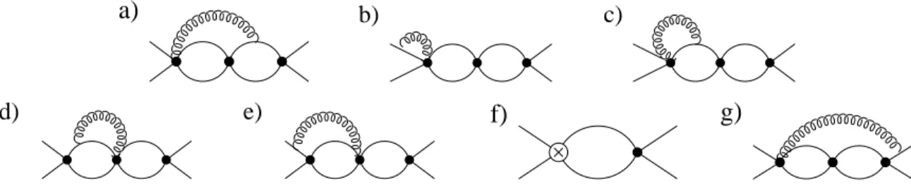
d) e) f) g)

FIG. 7. Graphs with ultrasoft gluons which do not contribute to the running of the Coulomb potential. The divergences in a)-e) are canceled by graph f) which has an insertion of the corre- spondingVk counterterm(s) denoted by⊗. Graph g) is UV finite.

in the effective theory graphs.³ In the full theory at two loops there are no contributions proportional to 1/k²from off-shell regions. The soft effective theory graphs are UV divergent, however these divergences are in one-to-one correspondence with UV divergences in the full or static theory. Finally, the graphs with iterations of potentials are UV finite.

V. THREE-LOOP RUNNING OF Vc

To compute the three-loop anomalous dimension for the Coulomb potential we need to evaluate the UV divergent graphs in the effective theory that are order α⁴_s/v. We begin by considering diagrams with an ultrasoft gluon. In Coulomb gauge we have graphs with p·A/m vertices as well as the coupling of ultrasoft gluons to the Coulomb potential from the operator [6]

L= 2iV_c^(T)f^ABC

k⁴ µ^2ǫ_Sµ^ǫ_Uk·(gA^C)ψ_p^†′ T^Aψpχ^†_−p′ T¯^Bχ−p. (23) All graphs with two p·A vertices are UV finite or are canceled by two loop graphs with insertions of the one-loop counterterms for V2 and Vr computed in Ref. [4]. The remaining diagrams are shown in Figs. 7 and 8. Graphs 7a through 7e have UV subdivergences which are exactly canceled by the diagram with Vk counterterms shown in Fig. 7f. These graphs contain subdivergences that were responsible for the running of the 1/(m|k|) potential at two-loops [6]. Graph 7g is UV finite.

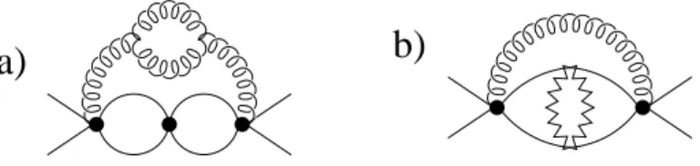
The divergent diagrams with an ultrasoft gluon which are not completely canceled by a counterterm diagram are shown in Fig. 8. Consider the three-loop graph in Fig. 8a with

3An example where UV divergences in the effective theory affect the matching is the two- loop coefficient for the production current.

a) ^{b) c)}

FIG. 8. Graphs with an ultrasoft gluon which contributes to the three-loop running of the Coulomb potential.

momental for the loop with the ultrasoft gluon andk and q for the remaining loops. After performing the k⁰ and q⁰ integrals by contours, the loop integration involving l is

Z

d^dl δ^ij −lⁱl^j/l²

l²(l⁰+E−k²/m)(l⁰+E−q²/m). (24) From this expression we see that the ultrasoft momentum l and potential momentum, k and q, are not completely separable since they appear in the same propagator. The l integration produces an UV divergence while the remaining integrations are UV and IR finite⁴. Evaluating the remaining integrals gives

Fig. 8a = 4i 3(C8a)

hV_c^(T)(ν)ⁱ³αU(ν)µ^2ǫ_S (4π)³k²

1

ǫ + lnµ²_U E²

+ 2 lnµ²_S k²

+. . .

, (25)

where the color factor is

(C8a) =CAC1

(CA+Cd)

8 1⊗1 +T ⊗T¯

, (26)

and for gauge group SU(Nc),Cd=Nc−4/NcandC1 = (N_c²−1)/(4N_c²). The graph in Fig. 8c involves the iteration of a 1/k² potential and a Vk counterterm and also has a Coulombic infrared divergence. This graph cancels the corresponding product of IR and UV divergences arising in Fig. 8b. The sum of graphs in Fig. 8b,c still has an UV divergence, and we find

Fig. 8b + 8c =−4i 3(C8bc)

hV_c^(T)(ν)ⁱ³αU(ν)µ^2ǫ_S (4π)³k²

1

ǫ + lnµ²_U E²

+ 2 lnµ²_S k²

+. . .

, (27) where the color factor is

(C_8bc) =CA

C₁(CA+Cd)

8 1⊗1−C₁+(CA+Cd)² 32

T ⊗T¯

. (28)

The sum of divergences in Eqs. (25) and (27) are canceled by a three-loop counterterm for Vc. Differentiating with respect to lnµS and lnµU gives the anomalous dimensions

4For static quarks this three-loop graph also has an IR divergence [18], but in the non-static case we find that this divergence is regulated by the quark kinetic energy.