14 Lagrangian Models

14 Lagrangian Models

14.1 Absolute and Relative Diffusion

In chapter 12 the ‘plume’ has been introduced (Fig. 12.2) and later described (for an ideal setting) according the theory of Taylor. Still, when observing plumes form real stacks (Fig. 14.1) they hardly look similar in most cases – the exception being maybe very stable conditions. The difference appears not so much from the idealising assumptions behind the theoretical plume, but rather from the fact that the two are not referring to the same. Figure 14.1 shows an instantaneous plume – every second later (or before) one would see a slightly modified plume. If one would overlay, then, all these instantaneous plumes the result would be a ‘mean plume’ and this is exactly what Fig. 12.2 shows. The difference is due to the turbulent nature of the PBL, which is to some degree random, but can be successfully described using statistical approaches (see Chapter 3).

Figure 14.1 Instantaneous plume from an industrial site

Consider an emission from a point source: all ‘tracer particles’ (i.e., all fluid elements that we have ‘marked as tracer’) will at first experience the same local flow and turbulence characteristics. Their evolution will therefore initially not be independent of each other. If this ‘young plume’ is carried away by an eddy that is larger than the momentary size of the plume, the entire plume is affected. This (large) eddy will not contribute to the growing of the plume. Small eddies, on the other hand, will not move the plume as a whole but will help it to grow.

Close to the source (when the plume itself is small) eddies of most

sizes will move the entire plume and only the smallest contribute to its

growing. The farther away the plume from the source (i.e., the larger

it has become) the more eddies are smaller than the plume itself, and

hence contribute essentially to plume growing. If we wanted to model

this behaviour on a ‘particle basis’, i.e. conceptionally taking each

particle into account, this would mean that close to the source any two particles in the plume are dependent – if one moves up also the other moves up, because the eddy has moved the entire plume up.

The relative dependence of any two-particle pair will weaken with increasing time (distance) from the source when increasingly larger eddies become smaller than the plume itself and may modify only parts of the plume. In terms of particle dispersion models, this is called ‘two-particle statistics’. The process being modelled in this way is called relative diffusion. One of the first to point out the fundamental difference between absolute and relative diffusion was Richardson (1926). If a sufficiently large number of instantaneous (or

‘relative’) plumes are overlaid, we have noted above that the result is a mean plume (Fig. 14.2). Thus in this picture the combined dispersing effect from eddies of all sizes are taken into consideration at all times. Again considering the ‘particle view’, this means that each particle can be treated as independent from all the others: the overall (mean) turbulence characteristics, in which the plume is growing determines the overall (mean) characteristics of the plume.

This is what we call absolute diffusion. Table 14.1 contrasts the two views on dispersion and gives typical applications.

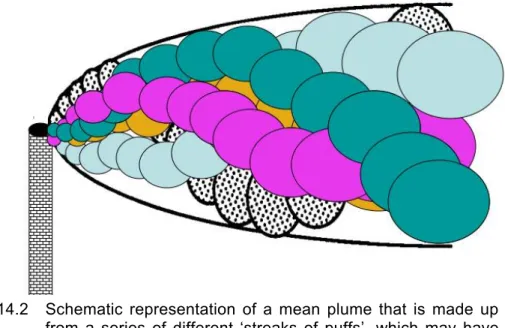
Figure 14.2 Schematic representation of a mean plume that is made up from a series of different ‘streaks of puffs’, which may have been emitted at consecutive times. Modified after de Haan and Rotach (1995).

14.2 Puff Models

One might view puff models as the ‘answer to plume model’s

deficiencies’. First of all, plume models always yield mean

concentration distributions and thus cannot take into account variable

(non-stationary) conditions. Also, ‘average’ concentration distributions (absolute diffusion) may not be very helpful if the risk potential should be assessed in an emergency preparedness system. Consider, for instance, a chemical plant that in case of an accident might release toxic substances. The evacuation plan should be based on the actually happening realisation (relative diffusion) of the dispersion process – and not on some mean downwind concentration distribution.

Table 14.1 Characteristics of absolute and relative diffusion

Absolute Diffusion Relative Diffusion

Plume Mean plume Single realisation

Fluid elements Independent Dependent

Particle statistics One-particle statistics Two-particle statistics Application Mean concentrations Instantaneous

concentration (e.g., yearly average,

environmental impact assessment)

(e.g., emergency response system

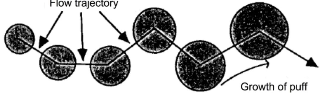
A puff model is very simple in principle. Every time unit a portion of the pollutant is emitted as a ‘puff’. Its initial size is larger than zero, most often the size of the exhaust pipe or the chimney. After release the puff follows, on the one hand, the flow trajectory and grows on the other hand (Fig. 14.3). The flow trajectory may thereby stem from a simple (even one-dimensional) parameterization as the one extreme, or a frequently updated three-dimensional field from a numerical model on the other side of the spectrum. Clearly, the typical application of puff models – emergency response systems – would prevent from using a too sophisticated flow model just for reasons of computational efficiency.

Figure 14.3 Schematic of a series of puffs following a flow trajectory

thereby growing. Modified after de Haan and Rotach (1998).

The central problem in any puff model consists, of course, in describing the relative diffusion. From the discussion in section 14.1 (see also Fig. 14.2) it is clear that

€

σ

(t ) < σ

(t) due to the fact that the large eddies do not contribute to

€

σ

^{but to}

€

σ

^{. For} practical reasons it is usually assumed that the concentration distribution in all coordinate directions is usually assumed to be Gaussian. This is not very problematic an assumption, except maybe very close to the surface. An appropriate description of puff growth requires two-particle statistics, which typically address a question of the type: ‘if two particles have the distance

€

r

at time

€

t

, what is the probability their relative distance at time

€

t

+ Δ t to be

€

r

+ Δ r (where we have omitted the vector notation for the space allocation for simplicity)?’ A thorough review of tow-particle approaches can be found in, e.g., Borgas and Sawford (1994). Mikkelsen et al. (1987) discuss a wealth of different approaches, on how to use two-particle statistics in order to model the rate of growth of the puff. The simplest of these goes back to Smith and Hay (1961)

€

d σ

dx = 0.22I , I =

σ

i=1,3

∑

u

^(14.1)

where

€

I is the turbulence intensity (3.26), based on the total turbulent energy. We note that for stationary and homogeneous turbulence

€

σ

grows linearly with distance from the source (or with time, using Taylor’s hypothesis).

Similar to plume models do puff models have a problem with mass conservation once the puff has grown to the size of the domain (in the horizontal) or the PBL height (in the vertical). The usual approach is then ‘furcate’ the puff (e.g., Thykier-Nielsen et al. 1989) into several new puffs. In a trifurcation, for example, the original puff is replaced by 3 new puffs. These new puffs have half the size of, and are placed half a standard deviation apart from the original puff; also one new puff is placed at the original location itself. The masses of the new puffs are chosen such that the new total density distribution (of the three furcated puffs) is as similar as possible to the distribution of the original puff.

Two applications may illustrate typical scenarios for puff models.

A) One emitted puff: this case corresponds to the release of a pollutant puff, e.g., in connection with an accident in a chemical plant. The sequence of puffs will then be as in Fig.

14.3, but only if a sufficiently resolved (in time and space) and

sophisticated flow field is available. If this were the case the

dispersion model would also be able to cover horizontal

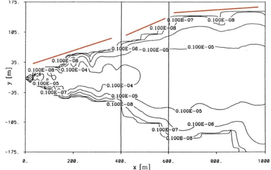
inhomogeneity such as the reaction of the puff travelling over the roughness transition from a lake to the shore (Fig. 14.4).

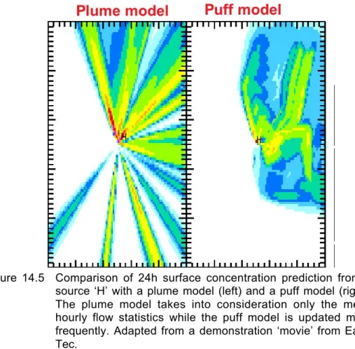
B) Series of emitted puffs: This situation corresponds to a continuous source. Again the flow and turbulence field must have a sufficient resolution in order to simulate a reasonable (mean) concentration distribution (Fig. 14.2). However, even with a low temporal resolution (one hour, say) the features of the flow and turbulence field in complex topography may render the result from a puff model far more realistic than those from a plume model (Fig. 14.5).

Figure 14.4 Simulated pollutant distribution form a source near the surface over an inhomogeneous surface. The stripe between 400m and 600m downwind of the source has a surface roughness that is 50 times larger than in the rest of the domain. The red lines indicate the changing dispersion characteristics. Modified after de Haan and Rotach (1995).

Over all it turns out that puff models are appropriate when high-

resolution flow and turbulence fields are available and also

necessary, this is in complex terrain; and when instantaneous

concentrations are required (emergency response systems).

Figure 14.5 Comparison of 24h surface concentration prediction from a source ‘H’ with a plume model (left) and a puff model (right).

The plume model takes into consideration only the mean hourly flow statistics while the puff model is updated more frequently. Adapted from a demonstration ‘movie’ from Earth Tec.

Lagrangian Particle Dispersion Models

The approach of particle dispersion models is appropriate if the mean concentration distribution is required and the turbulence/flow field is strongly inhomogeneous and/or non-Gaussian. The latter is the case in the convective boundary layer where large thermals (Fig. 1.9) produce a skewed vertical velocity distribution (see Fig, 3.2), or within vegetation canopies. Alternatively, particle models may be employed using two-particle statistics (Borgas and Sawford, 1994, Thompson, 1990) in order to estimate concentration fluctuations, again for complex flow situations. The prerequisite for Lagrangian particle dispersion models (LPDM’s) is the same as for puff models. It is assumed that the turbulence and flow fields are ‘given’ – either from parameterisations or numerical modelling. Into this environment a

‘large’ number ( O (

€

10

− 10

)) of particles is emitted from the source location. They all follow the mean trajectories on average but each particle has its own individual path due to the turbulent nature of the flow. These individual paths are partly dependent on the particle’s

‘history’ (i.e., the flow’s auto-correlation field

) and to some extent due

1

In fact, LPDMs are modelled as auto-regressive (AR) processes. In AR processes

the state n+1 of the system is determined from states n, n-1, …1. An AR process of

first order uses only state n (present) to predict n+1 (future). All AR processes of

order one and zero are called Markov Processes and have some convenient

to a stochastic component. These correlated and random contributions to particle acceleration at anyone instant in time must be modelled in such a way that on average (over all particles) the velocity field of the particles corresponds to that of the flow. In other words it is assumed that the particles behave like fluid elements. For each particle then, and at each time step, a LPDM consists in calculating the individual acceleration that allows for determining an updated position. Concentrations may – in the simplest approach – be determined from counting particles in predefined boxes.

14.3.1 Model formulation

A general formulation for the description of the change in velocity component

€

u

over a time step

€

dt is a so-called generalised Langevin equation and reads

€

du

= a

( x r , u r ,t)dt + b

( x r , u r ,t )d ξ

(14.2) Here

€

a

and

€

b

are two yet unknown functions of time, space and the present velocity and

€

d ξ

is the so-called increment of a Wiener Process. For the present purpose it is enough to state that a Wiener Process is a random process, the realisations of which have zero mean and variance

€

dt . To put it simple:

€

d ξ

is a random number with the condition that all these random numbers together have zero mean (

€

d ξ

= 0 ) and variance

€

dξ

= dt . For each of the particles and for each time step eq. (14.2) is evaluated in order to obtain an updated velocity and the updated position follows from

€

d x r = u dt r (14.3)

In (14.2) the functions

€

a

describe the correlated part of the acceleration while

€

b

are responsible for its random (stochastic) part.

Over all, these functions must be determined in a way that ‘the turbulence statistics are right’. For a long time research on LPDMs mainly consisted in finding appropriate criteria for the process (14.2) so that an explicit formulation of the model functions

€

a

and

€

b

was possible. In Section 14.3.3 we will consider some of these in order to see what is meant by ‘the statistics are right’. However, Thomson (1987) has analyzed several selection criteria for such models and has shown that they are all equivalent or weaker than the well-mixed condition (WMC). This condition requires, simply speaking, that particles initially well mixed in position- and velocity-space remain well mixed after a long application of the model.

The WMC for the Markov Process (see Footnote 1) specified by (14.2) can be expressed by taking advantage of the fact that, under

statistical properties. An important prerequisite in the derivation of LPDMs is that

the Markov property is assumed.

well-mixed conditions, the pdf of the particle velocities,

€

P

, is equal to that of the Eulerian velocities of the flow, here denoted as

€

P

. The Fokker - Planck equation

for process (14.2) reads as follows

€

dP

dt = − ∂

∂ x

(u

P

) − ∂

∂ u

(a

P

) + ∂

∂ u

∂ u

(B

P

) (14.4) where

€

B

= 1 2 ⋅ b

b

is an abbreviation. Following Thomson (1987), (14.4) can be re-written for stationary turbulence as

€

a

P

= ∂

∂u

(B

P

) + Φ

, (14.5)

where

€

Φ

obeys

€

∂Φ

∂u

= − ∂

∂x

(u

P

) , (14.6)

with the restriction on

€

Φ

that

€

Φ

→ 0 for

€

u v → ∞|. Thus with (14.5) and (14.6) the WMC allows to devise an LPDM if the (Eulerian) velocity pdf of the flow is known (and allows for a solution to 14.5 and 14.6, of course).

Equations (14.5) and (14.6) allow for a unique solution in the one- dimensional case. However, from (14.6) it is apparent that, for descriptions of the flow in more than one dimension, the solution for

€

Φ is not unique: for every

€

Φ solving (14.6) there exists an infinite number of

€

Φ

, which are solenoidal in u-space (

€

∂ Φ

∂ ^u

= 0), so that

€

Φ + Φ

is also a solution to (14.6). Sawford and Guest (1988) have demonstrated that the problem of non-uniqueness is indeed non- trivial

and several authors have proposed additional criteria (e.g., the

‘rotation of trajectories’ due to Sawford 1999 or the ‘trajectory curvature’ due to Wilson and Flesch 1997, also Reynolds 1998). Still, at the time of writing (2006) no generally accepted criterion (additional to the WMC) has been devised for LPDMs.

Thomson (1987) has constructed the simplest (his wording) LPDM based on the WMC, that is, the situation of (stationary) Gaussian correlated turbulence. Hence the pdf is described according to

€

P

= 1

2 π

( )

^{(det V)}

exp − 1

2 u'

V

u'

 



 

 , (14.7)

2

The Fokker-Planck equation can be viewed as a ‘conservation equation for the velocity pdf’ and is specific to the formulation of the AR process (eq. 14.2 in our case). In deriving the Fokker-Planck equation it is instrumental to assume the Markov property.

3

Basically they have shown that two different solutions indeed yield different

concentration fields.

where

€

V

is the Gaussian covariance matrix (essentially corresponding to the Reynolds stress tensor, 3.22) and

€

det V its determinant. Thomson’s ‘simplest solution’ then reads

€

a

= −B

(V

)

u'

+Φ

/ P

, where

Φ

P

= 1 2

∂ V

∂ x

+ ∂ u

∂ t + u

∂ u

∂ x

+ 1

2 ( V

)

∂ V

∂ t + u

∂ V

∂ x



  

  + ∂ u

∂ x



 



  u'

+ 1

2 (V

)

∂V

∂x

u'

⋅ u'

(14.8)

14.3.2 The random acceleration

The increments of the Wiener Process must not be correlated among each other for different coordinate directions and times

€

d ξ

(t )d ξ

(s) = δ

δ ^(t − s)(dtds)

. (14.9) Also it is advantageous if

€

d ξ

are not correlated with the functions

€

a

. In order to find a suitable formulation for the ‘random functions’,

€

b

, we recall the Lagrangian structure function for a velocity component (cf. eq. (7.14))

€

D

i

( Δ t ) = ( u

'(t ) − u

'(t + Δ t )

^{= ( Δ u}

⁾

^{. (14.10)}

If the time increment is such that the corresponding frequency lies in the inertial subrange (see Chapter 7), the structure function can be described according to

€

D( Δ t

) = C

εΔ t

, (14.11)

where

€

C

is a universal constant and

€

ε the dissipation rate of TKE.

The incremental form of (14.2) reads

€

Δu

= u

(n + 1) − u

(n) = a

Δt + b

Δξ

^(14.12) and can be multiplied with itself and averaged over many realisations:

€

(Δu

)

= a

Δt

+ 2a

b

ΔtΔξ + b

Δξ

. (14.13) The middle term on the rhs of (14.13) is zero due to the condition that

€

d ξ

= 0 . Also the first term on the rhs must be zero since the state

n+1 evolves from state n and a random process has been involved in

this transition. Therefore the two states must be statistically

independent

. Comparing (14.10) and (14.13) – for the time increment in the inertial subrange – therefore yields

€

( Δ u

) = b

Δξ

= C

εΔt ^(14.14) or

€

b = (C

ε ⁾

_(14.15)

where we have dropped the subscripts for convenience and have used the mean value for the variance of the Wiener Process’

increment. There is considerable uncertainty in the value for the

‘Kolmogorov constant’

€

C

with values ranging from 1.5 to about 10.

Recent estimates (Du et al 1995, Rotach et al. 1996, Anfossi et al.

2000) suggest a value around

€

C

= 3 − 4 for a wide range of applications. Equation (14.15) is a very convenient result as the function

€

b turns out to be equal for all coordinate directions and independent from the velocity itself. This simplifies the search for the correlated contributions to the acceleration (functions

€

a

) considerably (see below). The only limitation is the time step, which needs to lie within the inertial subrange.

In the (early) literature an alternative description for the function

€

b can often be found:

€

b = ( 2 σ

T

)

(or

€

C

ε = 2 σ

T

) (14.16)

This formulation is only valid for stationary and homogeneous Gaussian turbulence as the following derivation shows. Formally the structure function can be written

€

D

( Δ t) = C

εΔ t

= u

(t ) − u

(t + Δt )

= u

(t ) + u

(t + Δ t ) − 2u

(t ) ⋅ u

(t + Δ t)

= 2 σ

(1 − R

( Δ t ))

(14.17)

where we have used the definition of the auto-correlation function (3.27) and substituted

€

Δt for

€

τ . Also we have used that in stationary turbulence

€

u

(t) = u

(t + Δ t) = σ

. Expanding the simple approach for the auto-correlation function (3.29) into a Taylor series around

€

Δ t = 0

yields (up to the linear first term)

€

R

( Δ t ) ≈ 1 − Δ t

T

^{, (14.18)}

4

Mathematically, to comprehend this argumentation, one must be aware that eq.

(14.2) cannot be integrated in a Riemann sense. Integration rules for stochastic

differential equations are defined in the so-called Itô calculus.

so that inserting (14.18) into (14.17) yields the result (14.16).

14.3.2 Two Simple, one-dimensional LPDMs

In this section some of the simplest LPDMs are presented – mainly for pedagogical reasons. In any case, the presented solution can be verified by inserting the velocity pdf according to the specifications into the Fokker-Planck equation (14.4). Rather than doing this explicitly we demonstrate (following de Baas, 1988) some of the properties of the chosen model in order to show how criteria have been sought (before the WMC) to find the model functions

€

a

. For simplicity we only consider one-dimensional models for the vertical velocity component and use the notation

€

u

= w ,

€

x

= z .

The simplest case to consider is of course stationary, homogeneous Gaussian turbulence (we first note that for this specification an LPDM is an ‘overkill’ in the sense that a simpler – faster – puff or even plume model would do it). As a model we consider

€

dw = − w

T

dt + ( 2σ

T

)

dξ . (14.19)

Thus we have employed (14.16) and

€

a = − w T

. Considering the discrete form we may write for state n+1

€

w

= w

+ Δ w

= (1 − Δt

T

)w

+ Δµ

= αw

+ Δµ

(14.20)

Here,

€

Δ µ is simply an abbreviation for the random term and variable

€

α is defined through (14.20). Due to stationarity and homogeneity

€

α = const. Now (14.20) is multiplied by

€

w

and the result can be divided by

€

w

= w

due to stationarity, yielding

€

w

w

w

= α w

w

w

= α w

w

w

^{. (14.21)}

This exactly corresponds to the definition of the auto correlation function since the states n+1, n or n+1-k are separated by

€

τ = kΔt ^, i.e., discrete time steps:

€

R

(kΔt ) = αR

((k −1)Δt ) . (14.22) With the initial condition

€

R

(0) = 1 we finally have

€

R

(k Δ t ) = α

, 0 < α < 1, (14.23) where the constraint on

€

α follows from (14.21). For this range of

€

α it

can be shown that for large k

€

k

lim

Δt⋅k=const

(1 − Δ t

T

)

= exp − k Δ t T

 



 

 = R

( τ = k Δ t

T

) _(14.24)

(for this compare the Taylor series of

€

exp { − k Δ t T

} ^around

€

kΔt = 0 with that of

€

(1 − Δ t T

)

around

€

Δ t T

= 0 - and for the second the limit

€

k → ∞ ).

Thus we have shown that the model (14.19) yields a correct auto- correlation function (for the particle velocities) – and hence the model is valid. In a similar fashion one might also investigate the resulting spectral function or other statistical properties of a model like (14.19).

One may wonder whether the model (14.19) is also valid for Gaussian inhomogeneous turbulence (which is by far the more common case, especially in the vertical), i.e. whether it also fulfils the WMC under these conditions. In the neutral PBL (as an example) the vertical velocity variance decreases approximately linearly with height (Fig. 14.6). In our model (14.19) the vertical velocity variance only appears in the random part of the acceleration – all the other parameters are constant. Now, assume a situation in which the pollutant is already well mixed. Particles near the ground (large vertical velocity variance) will experience a large acceleration, hence a large velocity and quickly leave the region (on average). In contrary, at higher levels particles will not be accelerated as much and correspondingly remain (longer) in that region. Thus particles will concentrate in regions with small vertical velocity variance. Thus the model violates the WMC if

€

w

= w

(z)! For the case of Gaussian inhomogeneous turbulence, solution of the Fokker-Planck equation yields the following one-dimensional model

€

dw = − w T

+ 1

2 ( w

w

+ 1) dw

dz















 dt + (C

ε )

d ξ

. (14. 25)

In comparison to (14.19) there is an additional term that is proportional to

€

dw

dz and often referred to as ‘drift correction’.

Figure 14.6 Normalized vertical velocity variance under neutral conditions, where h (

€

≈ 2km ) corresponds to the height where the lateral velocity component is zero. Based on Large-Eddy simulation (Mason and Thomson, 1987). Modified after Stull (1988).

14.3.3 More Sophisticated LPDMs

In the preceding sections we have seen that the most general condition on a LPDM is the WMC. The corresponding Fokker-Planck equation allows to deriving the functions

€

a

(14.2) if the velocity pdf

for the flow under consideration is specified. Clearly, for this to work

the Fokker-Planck equation also must have a solution for the

specified pdf – and therefore the ‘art of devising an LPDM’ is to a

large extent that of finding an appropriate and mathematically benign

pdf, so that the Fokker-Plank equation can be solved. Different

approaches have been proposed such as the bi-Gaussian pdf (see

below) or the Gram-Charlier pdf (Anfossi et al. 1996). All the

approaches proposed so far have their specific advantages and

drawbacks so that the best model is usually that, which is based on

an approach, for which its drawbacks are not so relevant for the

problem under consideration.

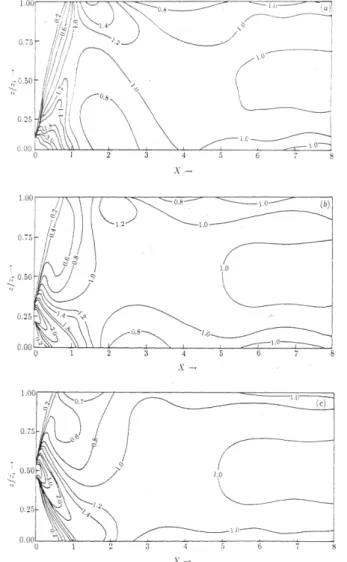
Figure 14.7 Laboratory convection tank results showing contours of non- dimensional crosswind-integrated concentration (CIC) as a function of dimensionless height

€

Z and downwind distance

€

X for sources at three heights in a convective boundary layer.

CIC is non-dimensionalised by

€

Q u z

; green horizontal arrows denote the release height

€

z

. (a)

€

z

z

= 0.067 , from Willis and Deardorff (1976); (b)

€

z

/ z

= 0.24 , from Willis and Deardorff (1978); (c)

€

z

/ z

= 0.49 , from Willis and Deardorff

(1981). The red dashed lines denote the approximate contour

of the maximum concentration. Modified after Weil (1988).

Here we consider an example of one and three-dimensional dispersion in the CBL with its characteristic skewed vertical velocity distribution (Figs. 1.9 and 3.2). For this situation the seminal water tank experiments of Willis and Deardorff (1976, 1978, 1981) have exhibited very characteristic pollutant distributions with a downwind development dependent on (relative) source height. To reproduce this has for quite some time been the challenge of particle dispersion modelling.

Figure 14.7 shows that for low sources in a CBL the concentration maximum remains close to the ground until it is lifted up at non- dimensional distance of approximately 1 (Fig. 14.7a). Pollutants emitted from higher sources will experience (on average) first a sinking motion (reflecting the higher probability of subsidence, Fig, 1.9) before they are lifted by a thermal (Figs. 14.7b,c).

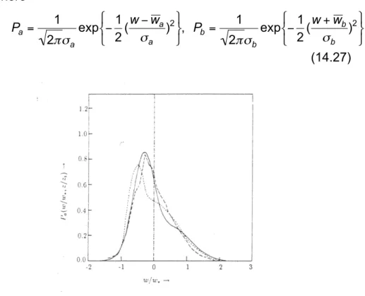
Luhar and Britter (1989) have proposed a one-dimensional LPDM for the CBL that is based on a skewed vertical velocity pdf, which is constructed from two Gaussian pdf’s according to

€

P

= AP

+ BP

_(14.26)

where

€

P

= 1 2 πσ

exp − 1

2 ( w − w

σ

⁾



 

 

 , P

= 1 2 πσ

exp − 1

2 ( w + w

σ

⁾



 

 

 (14.27)

Figure 14.8: Probability density function of the vertical velocity component in at

€

z / z

= 0.25 in a CBL. Dashed line: observation from

water tank (Willis and Deardorff 1978), solid line eq. (14.26)

with corresponding closure, dotted line another numerical

simulation, From Luhar and Britter (1989).

These two Gaussian distributions represent up- and downdrafts, respectively and the two Parameters

€

A and

€

B may be viewed as the area portion covered with them (Baerentsen and Berkowicz 1984).

Figure 14.8 shows the degree up to which a skewed velocity pdf (Fig.

3.2) can be approximated with (14.26). Inserting (14.26) into the Fokker-Planck equation (14.5) yields the full (and unique) solution (see Luhar and Britter, 1989, for details) that is able to reproduce the idealized water tank experiments (compare Fig. 14.7 and Fig. 14.9).

As a side product the model of Luhar and Britter (1989) yields (from the normalisation of the pdf) approximate values for the up- and downdrafts portion in the CBL:

€

A ≈ 0.36 and

€

B ≈ 0.64 .

Figure 14.9 As Figure 14.7, but modelled with a one-dimensional LPDM allowing for a skewed pdf in the vertical velocity. From Luhar and Britter (1989).

The model of Luhar and Britter (1989) shows how for a specific

problem – dispersion in the CBL – an appropriate model can be

constructed: in the CBL it is mainly the (skewed) vertical velocity,

which determines the concentration distribution and therefore one- dimensionality is not a real restriction. However, if such a model would be employed in, say, an emergency response system the Luhar and Britter model would only be appropriate for daytime conditions and during other conditions another model would be required. Rotach et al. (1996) and de Haan and Rotach (1998) have therefore constructed a full three-dimensional model that includes all possible boundary layer states. It is based on the following approach for the pdf

€

P

= Ψ P

P

P

+ (1 − Ψ )P

P

P

P

, (14.28) where

€

Ψ is a parametric function (see below) that ranges from zero (neutral to stable conditions) to one (convective conditions). The partial pdf's

€

P

, P

, P

are all Gaussian in the corresponding coordinate direction,

€

P

describes the (Gaussian) covariance distribution between vertical and longitudinal velocity component (

€

u' w' ) and

€

P

is according to (14.26). Thus under stable to neutral conditions (

€

Ψ = 0 ) the pdf is fully Gaussian, correlated between u’

and w’ and the model of Thomson (1987) (eq., 14.8) results as a solution. For convective conditions (

€

Ψ = 1 ), on the other hand, the turbulence is modelled to be skewed in the vertical velocity, with no correlation (

€

u' w' → 0 ). Figure 14.10 sketches this configuration.

Figure 14.10 Illustration of the hybrid pdf in the LPDM of Rotach et al.

(1996).

The full solution of the Fokker-Planck equation is rather lengthy (see the original papers by Rotach et al. 1996 and de Haan and Rotach 1998 for explicit formulations). The transition function

€

Ψ is apparently a function of stability and hence as arguments

€

z, z

and L were

chosen. Neutrality ( Ψ → 0 ) may either be reached if the heat flux

goes to zero, or if

€

z → 0 . Considerations on the mathematical behaviour of

€

Ψ (Rotach et al 1996) lead to the following constraints

€

lim

Ψ = δ , lim

w_*→0

Ψ = 0 (14.29)

Thus the following parametric function was proposed

€

Ψ = C

(C

− cos g) (14.30)

with

€

g = C

π (1 − exp { z / L) } ^{) (14.31)}

and

€

C

= 1− δ

2 , C

= 1+ δ

1− δ , δ = α

w

u

+ α

^{, (14.32)}

where the values

€

α

= 2.5 ⋅ 10

ms

and

€

α

= 10

ms

proved useful.

Finally, the parameter

€

C

is determined according to

€

C

= 1 − C

( u

w

)

(14.33)

and

€

C

= 1.65. Figure 14.11 depicts the height dependence of

€

Ψ ^for different stability conditions in the PBL. Figure 14.12 shows – as one result from this model – the excellent correspondence to the water tank results of Willis and Deardorff (in this representation the mean plume height and the vertical plume depth) that can be achieved with such an arguably quite computationally involved LPDM.

Figure 14.11 The transition function

€

Ψ in the model of Rotach et al (1996) describing the transition between Gaussian, correlated turbulence

€

Ψ = 0 and skewed in the vertical velocity but uncorrelated turbulence

€

Ψ = 1 , for three cases of stability D:

ideally neutral (dotted line); C: forced convection (dashed

line), B: highly convective (full line). From Rotach et al (1996).

14.3.4 Practical issues with LPDMs

In this section a number of practicalities in connection with LPDMs are addressed and some useful references are given.

Particle Reflection

For short range dispersion problems particles are confined to the boundary layer or, in other words, ‘reflected’ at the ground (

€

z

> z

) and at the boundary layer height. Reflection is often simply modelled as mirroring the particle position at

€

z

and

€

z

, respectively and inverting its vertical velocity component once a particle has gone beyond one of these limits within a time step. Thomson and Montgomery (1994) show that this ‘perfect reflection’ is only appropriate for Gaussian turbulence and investigate some alternative methods for the case of non-Gaussian turbulence. Rather than explicitly reproducing them here, we only mention that they are rather

‘unfriendly’ to use in that they require pre-calculated ‘lookup tables’ to

satisfy the statistical requirements. In addition, Thomson and

Montgomery (1994) note that if the time step is ‘small enough’ near

the boundary (which is often the case for other reasons in non-

homogeneous turbulence, see below), the WMC can be maintained,

no matter which reflection criterion is applied.

Figure 14.12: Comparison of mean plume height (left column) and vertical plume spread (right column) between the model of Rotach et al (1996), solid line, and the water tank observations of Willis and Deardorff (1974, 1976, 1981), black dots. Top row:

release at

€

z / z

= 0.49 , middle row: release at

€

z / z

= 0.24 , lower row: release at

€

z / z

= 0.067 .

Concentration estimates

Pollutant concentrations are, in principle, easily determined from LPDM output. For a given source strength in

€

[gs

] each particle is attributed its ‘share’ of the pollutant mass and the model domain can be divided into boxes where particles are counted and the concentration determined. This approach is widely used and harmless in principle. However, if steep concentration gradients are to be reproduced (e.g., close to the source or close to the ground) the

‘box counting’ approach requires very small boxes (and hence huge amounts of particles) in order to obtain smooth concentration distributions. Figure 14.12 illustrates the effect on concentration estimates when using too few particles (with a given box size). In order to circumvent this problem, de Haan (1999) has proposed a so- called density kernel estimator, according to which the concentration

€

c from

€

n particles of equal mass is estimated from

€

c( x r ) = 1 nh K

i=1 n

∑ ( x r − x r

h ) , (14.34)

where

€

h is the width of the kernel and

€

K is the kernel function (normalised to one). Thus this approach corresponds to attributing a

‘density distribution’ to each particle (rather than a ‘delta peak’). The most important parameter of this estimate is the bandwidth (

€

h ) since it plays the role of a smoothing parameter. De Haan (1999) discusses various kernel functions and appropriate choices for

€

h . As can be

seen from Fig. 14.12 does the kernel estimator allow for a smooth

and ‘true’ concentration distribution, even if relatively few particles

(5000, in this case) are simulated.

- 21 -

Figure 14.13 Concentration estimates in a numerical experiment (stability of forced convection) with a release height at

€

z / z

= 0.025 . The long-dashed line (– – –) shows the box counting prediction for vertical and horizontal box sizes of 0.05 zi. The short-dashed line (---) is for vertical and horizontal sizes of 0.005zi. Both simulations employ only 1000 particles. The thick line (–– ) depicts the ‘‘true’’ concentration (100’000 particles). The thin solid line (–) shows the concentration prediction using a recommended kernel method. From de Haan (1999).

Time step criteria

In connection with eq. (14.15) we have noted that the time step must be chosen such that its corresponding frequency lies in the Inertial Subrange. However, this condition is not always sufficient in order to allow for smooth particle tracks. Thomson (1987) has noted that additional constraints are needed in order to ensure that a particle cannot have too large a fractional change in phase space over a single time step. The problem can best be understood when considering (14.5) in order to seeing that the functions

€

a

are complicated ratios of complicated (in general) functions that can easily go ‘to infinity’ if one or the other approaches zero faster than the other (for large velocities, hence small probabilities). Some authors have proposed to simply ‘cut’ the pdf at a certain threshold (e.g. Luhar and Britter, 1989). Another approach has been proposed by Rotach et al. (1996) who have extended Thomson’s criteria to yield

€

dt

= min( 0.01 σ

B , 0.1 σ

a

, 0.01 σ

u

∂σ

/ ∂x

, 0.01 ε

u

∂ε / ∂x

) (14.35) Using these criteria it is most convenient to define a default time step,

dt

say that is relatively large. For each particle then, each coordinate

direction and each time step (14.35) is evaluated. If

€

dt

< dt

, the former is used (which is usually the case in most of the domain). If

€

dt

> dt

on the other hand,

€

dt

is used (for that particle only) first, and a new velocity and position are calculated. Then (14.35) is evaluated again, and a new

€

dt

is determined. This procedure is repeated until the sum of incremental sub-time steps equals the default

€

dt

(so that the particle under consideration has the same time as all the others. With this approach one can avoid to prescribing very small time steps (what is cpu time consuming) without the requirement to cut the velocity pdfs at an arbitrary threshold.

References

Anfossi D, Ferrero E, Sacchetti D and Trini Castelli S: 1996, Comparison among empirical probability density functions of the vertical velocity in thes surface layer based on higher order correlations, Boundary-Layer Meteorol, 82, 193- 218.

Anfossi D, Degrazia G, Ferrero E, Gryning SE, Morselli MG and Trini Castelli S:

2000, Estimation of the Lagrangian Structure function constant Co from surface layer wind data, Boundary-Layer Meteorol, 95, 249-270.

Baerentsen J and Berkowicz R: 1984, Monte Carlo simulation of plume dispersion in the convective boundary layer, Atmos Environ 18, 701-712

Borgas MS and Sawford BL: 1994, A family of stochastic models for two particle dispersion in isotropic homogeneous stationary turbulence. J Fluid Mech, 279, 69-99

De Baas AF: 1988, Some properties of the Langevin model for dispersion, Risø-M- 2627, Risø National Laboratory, Roskilde, Denmark, 232pp.

de Haan, P and Rotach, MW: 1995, 'A Puff-Particle Dispersion Model', Int. J.

Environment and Pollution, 5, Nos. 4-6, 350-359.

de Haan P and Rotach MW: 1998, A Novel Approach to Atmospheric Dispersion Modelling: The Puff-Particle Model, Quart J Roy Meteorol Soc, 124, 2771–2792.

Du S, Sawford BL, Wilson JD and Wilson DJ: 1995, A determination of the Kolmogorov constant (Co) for the Lagrangian velocity structure function, using a second-order Lagrangian stochastic model for decaying

homogeneous isotropic turbulence. Phys. Fluids, 1, 3083-3090 Luhar A and Britter RE: 1989, A random walk model for dispersion in

inhomogeneous turbulence in a convective boundary layer, Atmos Environ, 23, 1911-1924.

Mason PJ and Thomson DJ: 1987, Large-eddy simulation of the neutral-static

stability Planetary Boundary Layer, Quart J Roy Meteorol Soc, 113, 413-443.

Mikkelsen T, Larsen SE and Pecseli HL: 1987, Diffusion of Gaussian puffs, Quart J Roy Meteorol Soc, 113, 81-105

Richardson LF: 1926, Atmospheric diffusion shown on a distance-neighbour graph, Proc. R. Soc., London A, 110, 709-737.

Reynolds AM: 1998, On trajectory curvature as a selection criterion valid for Lagrangian stochastic dispersion models, Boundary-Layer Meteorol, 88, 77- 86.

Rotach MW, Gryning, SE and Tassone C: 1996, A Two-Dimensional Lagrangian Stochastic Dispersion Model for Daytime Conditions, Quart J Roy Meteorol Soc, 122, 367–389.

Sawford BL and Guest FM: 1988, Uniqueness and Universality of Lagrangian Stochastic Models for Turbulent Dispersion, Proc. 8th Symp. Turb. Diff., AMS, San Diego, CA. pp. 96–99.

Sawford BL: 1999, Rotation of trajectories in Lagrangian stochastic models of turbulent dispersion, Boundary-Layer Meteorol, 93, 411-424.

Smith FB and Hay JS: 1961, The expansion of clustersof particle in the atmosphere, Quart J Roy Meteorol Soc, 87, 82-101.

Stull RB: 1988, An introduction to Boundary Layer Meteorology, Kluwer, Dordrecht, 666pp.

Thomson DJ: 1987, Criteria for the selection of stochastic models of particle trajectories in turbulent flows, J Fluid Mech, 180, 529-556.

Thomson DJ: 1990, A stochastic model for the motion of particle pairs in isotropic high-Reynolds number turbulence, and its application to the problem of concentration variance, J Fluid Mech, 210, 113-153.

Thykier-Nielsen S, Mikkelsen T, Larsen SE, Troen I, de Baas A, Kamada R, Skupniewicz C and Schacher G: 1989, A model for accidental releases in complex terrain', In: Air pollution and its application VII, Ed. H. van Dop, Plenum Press, New York, USA

Weil JC: 1988, Dispersion in the convective boundary layer, in: Venkatram A and Wyngaard JC (Eds), Lectures on air pollution modeling, American

Meteorological Soc, Boston, 167-227.

Willis GE and Deardorff JW: 1976, A laboratory model of diffusion into the

convective planetary boundary layer, Q. J. R. Meteorol Soc., 102, 427-445.

Willis GE and Deardorff JW: 1978, A laboratory study of dispersion from an elevated source within a modelled convective planetary boundary layer.

Atmos. Environ,12, 1305-1311.

Willis GE and Deardorff JW: 1981, A laboratory study of dispersion from a source in the middle of the convective layer, Atmos Environ, 15, 109-117.

Wilson JD and Flesch TK: 1997, Trajectory curvature as a selection criterion for

valid Lagrangian stochastic dispersion models, Boundary-Layer Meteorol, 84,

411-426.