UseofNeuralNetworksforTriggeringintheBelleIIExperiment Masterarbeit Fakult¨atf¨urPhysik

Fakult¨ at f¨ ur Physik

LUDWIG–MAXIMILIANS–UNIVERSIT ¨ AT M ¨ UNCHEN

Masterarbeit

Use of Neural Networks for Triggering in the Belle II Experiment

von

Sebastian Skambraks

eingereicht am 18. Dezember 2013 bei:

Fakult¨ at f¨ ur Physik der

Ludwig-Maximilians-Universit¨ at M¨ unchen

Aufgabensteller:

Prof. Dr. Jochen Schieck

Prof. Dr. Christian Kiesling

Abstract

The trigger for the Belle II detector is a fast online event selection and data reduction mechanism where the interesting physics signal is selected for a later offline analysis whereas unwanted background is rejected. Since the full data rate generated by the detector will be too large to be recorded, triggering is a crucial component for the proper operation of the detector. Recent stud- ies have demonstrated the overwhelming power of the multi layer perceptron neural network approach in predicting the z-vertex position of single tracks.

Since the classical trigger methods lack in accuracy for this parameter, the neural networks could significantly enhance the signal to noise ratio in the collected data. This thesis investigates the relevance of background suppres- sion for the flavor factory Belle II together with the possible improvements of the neural network approach.

b

Contents

1 Introduction 1

1.1 Summary: “Use of Neural Networks for Triggering in Particle Physics” 3

2 Belle II Physics and Background 10

2.1 Physical Motivation for Belle II . . . 12

2.1.1 Flavor Physics in the Standard Model . . . 12

2.1.2 B Factories as Complementary Approach to the LHC . . . 16

2.2 Background in the Belle II Experiment . . . 20

2.2.1 Machine Properties . . . 20

2.2.2 Beam Induced Background Types . . . 21

2.3 Background Suppression with the Z-Vertex Trigger . . . 24

3 Conclusion 27 APPENDIX A 29 List of Abbreviations . . . 29

List of Figures . . . 30

List of Tables . . . 31

Bibliography . . . 32

Statement of Authorship . . . 34

APPENDIX B 35

Diploma thesis: “Use of Neural Networks for Triggering in Particle Physics” 35

c

d

1 Introduction

Following the successful results of the diploma thesis “Use of Neural Networks for Triggering in Particle Physics” [1], in this study the physics relevance of the neural network trigger is investigated. The anticipated future achievements in the flavor physics sector as well as the expected background situation for the Belle II detector are discussed. As a cumulative master thesis in physics, the full diploma thesis in informatics which was handed in on February 7, 2013 at the Institut f¨ ur Informatik of the Ludwig Maximilians Universit¨ at is attached to this document.

The Belle II detector [2] is a particle physics experiment that is currently in construction at the SuperKEKB collider [3] ring in Tsukuba, Japan. Like its prede- cessor, the Belle detector [4], it is a B factory, indicating its purpose to study the physics of processes involving b-quarks. The Belle detector which collected a data sample with an integrated luminosity of 1 ab

before its shutdown in 2010 [5], is now upgraded in order to achieve a higher luminosity and thereby a higher preci- sion in the measurements. With 8 · 10

cm

s

, the anticipated luminosity of the Belle II detector is ∼ 40 times higher than the luminosity in the Belle experiment.

However, the higher luminosity machine comes with new challenges, especially with respect to the background situation. The background in Belle II/SuperKEKB is expected to be much higher than the background in Belle/KEKB [6].

The main purpose of the Belle detector was to observe CP violation (

CP) in the

B meson system [5]. Major scientific breakthroughs were supported by the Belle ex- periment at the KEKB collider. The verification of the Standard Model (SM) quark flavor sector even led to the 2008 nobel prize for Kabayashi and Maskawa, who pro- posed the CKM mechanism in 1973 [7]. Many SM observables were measured with a high precision, and thereby limits for New Physics (NP) processes could be set [5].

With the higher luminosity, the Belle II detector will provide very high precision measurements of SM observables. This allows to further confirm the SM as the valid theory up to the GeV scale. Furthermore, indications of NP scenarios at the TeV scale can be measured with such a high precision machine. The NP processes are expected to have an effect on the loop corrections (higher order diagrams), and therefore a high precision measurement can give insight into physics beyond the standard model [8].

The main goal of the neural network studies is to start the implementation of a hardware component that can be attached to the Belle II level 1 trigger system as a z-vertex sub-trigger. In this study the z-vertex refers to the z-component of the position where a particle measured by the detector originated (i.e. it is a single track vertex) [1]. A big challenge for the new trigger subsystem will be the high requirements on the execution speed. The time window for the whole trigger sys- tem will be 5 µs [9], hence only ≈ 1 µs is left for this sub-trigger. Currently, an implementation on FPGA hardware is anticipated [1].

The z-component of the vertex is not yet provided by the other trigger com- ponents with a high accuracy [9]. Since the Belle II trigger is not yet constructed there exist no performance measures of the final trigger. However, at least some expectations can be inferred from the experience with the Belle experiment. After

1

several years of running of Belle the z-vertex still had the broad distribution shown in Figure 1. Only the narrow peak around z = 0 cm corresponds to the interesting physics signal, the whole side bands are background processes which were not re- jected by the trigger. Since the total background occupancy in Belle II will be much higher than in Belle, a similar or even worse situation can be expected. Therefore, a new z-vertex prediction method with an accuracy of . 2 cm could provide a drastic improvement of the signal to noise ratio in the collected data.

Figure 1: The z-vertex distribution of the data collected in Belle experiment No.

57. Source: [9, p. 366].

Neural networks have turned out to be very successful in solving various types of pattern recognition tasks [10] and they are also frequently used in particle physics analysis [11]. In the H1 experiment at the HERA collider, a hardware MLP neural network system was already used as a successful second level trigger [12]. From a theoretical perspective, for the 3 layer MLP there exists even a theorem prov- ing its capabilities to approximate any continuous function on the [0,1] hypercube [13]. Therefore, these studies are initiated and the capabilities of a neural network approach implemented as a z-vertex sub trigger in the Belle II trigger system are investigated.

The data from the Central Drift Chamber (CDC) is intended to be used as input for the neural network trigger.The CDC is a wire chamber with 14336 sense wires which are arranged in 9 cylindrical superlayers surrounding the beampipe and the IP [9]. A 3D reconstruction of charged tracks is possible via a stereo arrangement of the wires combined with the measurement of the distances of the tracks to the wires, the drift times. The drift time is the difference between the time the track ionized the initial gas molecules, and the time the pulse is measured at the sense wires. Due to the fairly constant drift velocity of the gas molecules, a track distance measure is given. The information provided by the CDC is a pattern of wires which were hit and a timing information for each hit. Starting from this input pattern, an efficient solution is required that can provide the z-vertex information sufficiently fast for the trigger system [1].

In the Subsection 1.1 the work of the diploma thesis “Use of Neural Networks for Triggering in Particle Physics” [1] is summarized and the main results are shortly

2

Figure 2: Components in the Belle II detector. Source: [14]

reviewed. In Section 2 the planned Belle II detector and its background situation are discussed. At first, Subsection 2.1 addresses the motivation for the Belle II experiments and therefore introduces the flavor physics sector within the SM. Next, the possible future achievements of the Belle II detector and its complementary role to the Large Hadron Collider (LHC) experiment is discussed. Secondly, Subsection 2.2 addresses the background production and suppression in the Belle II experiment.

The expected background types are reviewed and their relevance for a CDC based z-vertex trigger is discussed. Subsection 2.3 addresses the tremendous advantage of a z-vertex trigger for the Belle II experiment.

1.1 Summary: “Use of Neural Networks for Triggering in Particle Physics”

The diploma thesis “Use of Neural Networks for Triggering in Particle Physics” dis- cussed several machine learning approaches with focus on their ability to solve the z-vertex trigger task of the Belle II detector. Among the investigated methods were the Liquid State Machine (LSM) [15], the Elastic Arms algorithm (EA) [16] and the Multi Layer Perceptron (MLP) [10], [17]. In combination with a pre-processing step, the MLP finally provided the highest accuracy. Hence, it was chosen as a possible candidate for the Belle II trigger system.

3

The thesis begins with a chapter providing a detailed description of the trigger task that has to be solved by the neural network. The relevant detector compo- nent used as input, namely the CDC, and its geometry is described. Following, the trigger system with all its sub-trigger components is shown, in order to explain the position of the new neural network trigger within the signal flow of the trigger sys- tem. Furthermore, the difficulties in solving this z-vertex trigger task analytically are discussed which demonstrates the benefits of using a function approximation instead of calculating the actual function.

A theoretical background on common tracking methods in particle physics is summarized in chapter 3. The aim was to show fast algorithms used for tracking and to discuss, whether they could be used for the trigger system which demands an extremely short and deterministic runtime. Classic tracking methods like the Kalman filter, as well as new adaptive approaches like the EA algorithm are intro- duced.

After providing the general theoretical background, in chapter 4 the concrete methods used in the experiments and their implementation are documented.

At first this includes a general introduction on neural networks and the details on the three layer MLP implementation that is used to predict the z-coordinate as a floating point value.

Secondly, the important Look Up Table (LUT) method, which is the required pre-processor for the MLP is introduced. Based on a Bayesian parameter estimation the method can derive a proper phase space element corresponding to the hits in the CDC.

Another tracking method documented is the EA algorithm, an adaptive track finding algorithm. Starting from an initial track template, in an iterative procedure the track is “pulled” by the hits into the optimal position. After the introduction of the basic tracking algorithms, the corresponding meta-algorithms are shown. This is particularly the Resilent BackPROPagation (RPROP) algorithm, which was used for the training of the MLP (backpropagation) as well as for minimizing the cost function in the EA algorithm.

Additionally, a concept for the combination of the LUT and the MLP to a pre- diction chain is proposed: Starting from a coarse prediction of the track parameters, a specialized MLP can be selected that allows to predict the z-vertex value with a high accuracy.

In the 5th chapter experiments with the selected tracking methods described in chapter 4 are documented. Using simulated Belle II test data, the bias and variance of the methods were measured. The results allowed a discussion of their capabilities and usefulness for a z-vertex trigger. The following decision, which algorithms are combined into a prediction cascade, was made using these results.

Finally, the first experiments with the proposed prediction cascade are docu- mented in chapter 6. The LUT and the MLP are used combined: in combination with the 2D & 3D trigger input, the LUT provides the prediction of the track param- eters except z. On this basis a specialized MLP is selected which allows to predict the z-coordinate of the vertex position.

4

In order to review the main achievements, the results of some selected methods are now summarized and the experimental setup is outlined. The Monte Carlo data was generated within the software framework for Belle II (basf2). For the experi- ments single charged track events are generated, with restrictions on the five track parameters which are necessary to describe a helix shaped track. In the laboratory rest frame the common parameters to describe the tracks are: (z, d

, p

, φ, θ), where z is the distance of the vertex to the Interaction Point (IP) along the z-axis (beam pipe), d

is the distance of the track to the IP in the xy plane (distance of the vertex to the beam line), p

is the transverse momentum of the particle which is inverse proportional to its curvature, the angle φ describes the flight direction at the vertex within the xy plane, and θ describes the angle of the flight direction of the particle with respect to the z-axis.

By inspecting the correlation between the wires that were hit in the CDC and the track parameters, it can be observed that a small range in (p

, φ, θ) allows only a small subset of wires to be hit. The number of wires that are used as input for the neural network system can be heavily reduced by an a priori prediction of p

, φ, θ.

The main restriction will be given by p

and φ, which describe the curvature and orientation of the tracks projected into the 2D plane perpendicular to the z-axis.

In this projection the helix-tracks can be described by circles due to the magnetic field that is oriented along the z-axis. The angle θ will only slightly influence the selection of the stereo wires.

In the analysis phase, the precise value of d

is very important in order to recon- struct the life time of the B mesons, but for the trigger system this can be assumed to be approximately 0. Hence, a constraint in the parameters p

, φ, θ allows to fix all but the z-vertex value, and leaves this variable as the only one to be determined by the neural network.

The geometrical relation of these three parameters to subsets of wires in the CDC can be used in several ways. At first, for a sector specific neural network only this small subset of wires needs to be used as input. This ensures small network sizes that can easily be calculated. Secondly, this relation allows to extract the values of the three track parameters only by inspecting the hit pattern of the event. This approach is implemented in the Bayesian LUT.

In order to provide an overview of the results, next an experiment with single MLPs in a small subsector of the phase space (∆p

, ∆φ, ∆θ) is summarized. The z-vertex value of a track is the target value of the network. Using the geometrical constraint in p

, φ, θ only the geometrically reachable wires are used as input nodes.

The respective drift times at these wires are used as input values.

The concrete network in Figure 3 has a fixed number of input (20) and hidden (60) neurons, and one output neuron. Each neuron has the hyperbolic tangent as activation function. In order to meet the ranges of the tanh function, the input and output is scaled to lie within the region [−1, 1]. In the input layer each node corre- sponds to Track Segments (TS) of the drift chamber. By using a defined geometrical shape several wires are combined to a TS. They are generated in the trigger system in a first step in order to reduce the total number of signal wires and to perform a first noise suppression. The values provided as input to the MLP are the (scaled) drift time values measured at the reference wires of the active TS in the event. The value of the output node is interpreted as (scaled) z-vertex value.

5

a) b)

Figure 3: z-vertex prediction for fixed p

. θ ∈ [45, 46]

, φ ∈ [0, 1]

. a) p

= 7 GeV, σ = 0.9 cm. b) p

= 0.2 GeV, σ = 1.5 cm. Source: [1, p. 62].

The first results that show the capabilities of such a single MLP are shown in Figure 3. It shows the prediction of the z-vertex value by three layer MLPs. Two experiments are shown, one for a high momentum particle a), and one for a low momentum particle b). For the high momentum case of p

= 7 GeV, a z-vertex resolution of about 0.9 cm was achieved. For the low momentum case of p

= 0.2 GeV still a resolution of 1.4 cm was achieved. This demonstrates the capability of the MLP to solve the z-vertex trigger task, under the condition that some pre- knowledge on the track parameters is available.

p

∈ [0.2, ∞] GeV φ ∈ [0, 360]

θ ∈ [17, 150]

Table 1: Full CDC acceptance range for a single ionizing straight track originating from the IP. θ is constrained by the geometry of the CDC and p

has a lower bound due to the magnetic field. p

= 0.2 GeV is approximately the lowest transverse momentum required to hit all the layers of the CDC.

In order to construct a fully functioning z-vertex trigger, the full detector range in the variables (p

, φ, θ, z) has to be covered. The full CDC acceptance region for particles originating from the z = 0 cm is shown in Table 1. The approach proposed in [1] is to use many specialized MLPs and to combine them with a pre-processing step to select the correct MLP.

In [1] a coarse prediction was provided by combining the results of three meth- ods: a LUT providing a Bayesian parameter estimation, a coarse MLP which was not specialized to a subsector and as such had only a coarse resolution, and the prediction of the other trigger components (2D & 3D trigger system) were included.

The coarse MLP with its 4 output values was used to predict all track parameters (p

, φ, θ, z). The other trigger components provided (p

, φ) information by a 2D trigger and (θ, z) information by the 3D trigger.

The proposed Bayesian parameter estimation, the LUT, was implemented to model the relation between the hits in an event and the values of the variables (p

, φ, θ). The idea is, that it is possible to reverse the geometrical constraint in

6

(p

, φ, θ) which leads to a small subset of wires that are possibly hit in the event.

This means to infer the track parameters (p

, φ, θ) by identifying the sector in which the hits in an event are discovered. Like the MLP the LUT is a machine learning technique and is therefore trained with a training data set.

The LUT prediction can be described as a Bayesian parameter estimation of a track parameter vector S ~ = (p

, φ, θ)

, given a vector of hits of an event H ~ ∈ [0, 1]

. Each dimension is the hit-state of one of the 2336 track segments, which is either 1 or 0 because drift times are not used in this approach. The track parameter vector S ~ is binned in each variable, such that a sectorization of the phase space is given by S. The prediction with a LUT in terms of the Bayesian theorem reads: ~

P ( S| ~ H) = ~ P ( H| ~ S) ~ · P ( S) ~

P ( H) ~ (1)

where the probability distributions P can be thought of as histograms or n- dimensional matrices. The distribution P ( S| ~ H) allows to determine the probability ~ of a track parameter vector S ~ if the hit states vector H ~ is known. The distribution P ( H| ~ S) can be learned from a training data set, where the true track parameters are ~ known. The distributions P ( S) and ~ P ( H) provide a correction to the probability ~ value. In the LUT experiments conducted, they were assumed to be fairly constant and were therefore ignored [1]: only the relative highest probability is interesting for the track parameter estimation, not its absolute value. For a higher precision and the generalization to the full CDC acceptance region these corrections need to be taken into account.

p

∈ [1.5, 2.5] GeV φ ∈ [0, 11.25]

θ ∈ [40, 50]

z ∈ [−10, 10] cm

Table 2: Ranges of the track parameter sector, used in the simulated data set.

Source: [1].

In the experiments the distribution P ( H| ~ S) was modified after training. For each ~ sector the n

most relevant track segments (i.e. the ones with the highest probability to be hit in that sector) were determined. The probability values in P ( H| ~ S) were ~ then set to discrete values ∈ [0, 1]

: the top n

track segments got a 1, the others were set to 0.

Using this transformed histogram, the lookup was performed by summing P ( S| ~ H) ~ up all for all single hits in the event. The result was an a-posteriori probability distri- bution for P

( S) represented as an multi dimensional histogram. The most probable ~ sector S ~ and thus the prediction of the track parameters was found by peak-finding in the P

( S) histogram. ~

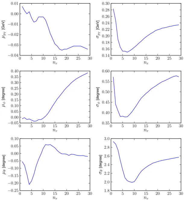
Representative results demonstrating the LUT capabilities in predicting the track parameters are shown in Figure 4. The LUT was constructed to predict the three track parameters p

, φ, θ using the dataset with the ranges listed in Table 2. The

7

0 5 10 15 20 25 30

n

−0.04

−0.03

−0.02

−0.01 0.00 0.01

µ

0 5 10 15 20 25 30

n

0.14 0.16 0.18 0.20 0.22 0.24 0.26 0.28 0.30

σ

0 5 10 15 20 25 30

n

−0.05 0.00 0.05 0.10 0.15 0.20 0.25 0.30 0.35 0.40

µ

0 5 10 15 20 25 30

n

0.35 0.40 0.45 0.50 0.55 0.60

σ

0 5 10 15 20 25 30

n

−0.25

−0.20

−0.15

−0.10

−0.05 0.00 0.05 0.10

µ

0 5 10 15 20 25 30

n

1.8 2.0 2.2 2.4 2.6 2.8 3.0

σ

Figure 4: Prediction bias and variance of a LUT predicting the track parameters (p

, φ, θ). The data contained simulated single track e

events with a uniform distribution of the track parameters with the ranges given in Table 2. For each track parameter the mean µ and the standard deviation σ were calculated on the deviation ∆x of the prediction to the real value: ∆x = x

− x

. Source: [1, p. 76].

histogram had 40 bins in φ, 40 bins in p

, and 5 bins in θ. The number of relevant track segments per sector n

(sector selection criterion) was varied in this experi- ment.

The accuracy was determined by inspecting the quantity ∆x = x

− x

for each variable x ∈ {p

, φ, θ}, and by calculating its mean µ and standard devi- ation σ. The standard deviations σ provide information on the possible resolution that can be achieved with this method. It is shown in the right column for various values of n

. The means µ provide information on the bias of the prediction method, they are shown in the left column. Since the interesting observable is the achievable resolution σ, these plots are drawn separately.

8

In Figure 4 a clear optimum in all variables is visible for 5 < n

< 10, which demonstrates the sensitivity to this parameter. The best accuracies are σ

≈ 0.16, σ

≈ 0.4

, σ

≈ 2

. This demonstrates the prediction capabilities of the LUT approach - one of the possible pre-processing steps required to select the correct MLP.

9

2 Belle II Physics and Background

The flavor physics experiment Belle II [2] is currently designed, with the goal to start taking data in 2016. It is placed around the IP of the SuperKEKB [3] collider ring.

In the SuperKEKB collider e

and e

particles will be accelerated with asymmetric beam energies of 3.5 GeV for the e

beam in the Low Energy Ring (LER) and with 8 GeV for the e

beam in the High Energy Ring (HER) [9]. The rest energy in the boosted Center of Momentum (CM) system corresponds to the Υ(4S) resonance, the fourth exited state of the b ¯ b meson with a mass of M

= (10.5794 ± 0.0012) GeV and a width of Γ

= (20.5 ± 2.5) MeV [18]. This resonance is chosen be- cause it has sufficient energy to allow a decay into two B mesons (Υ(4S) → B

B ¯

and Υ(4S) → B

B

). The Belle II detector will measure the decay products of the particles that are generated due to the collision in the IP, which allows various physics analysis of the different possible decay channels. In order to study heavy flavor physics involving b-quarks, the detector will be fine tuned to measure the expected physical processes. Due to the asymmetric beam energy the Υ(4S) will be generated with a boost along the z-axis, which allows to perform lifetime mea- surements by length measurements along the boost direction. To take care for the asymmetric production mechanism, the detector is constructed asymmetrically as well.

In the past, B factories like the Belle [19] and BaBar [20] experiments have con- tributed to the verification of the

CP and the flavor physics sector in the SM. It

was possible to provide experimental evidence for the correctness of the SM up to the GeV scale. By the high precision measurements, also bounds on new physics at the TeV scale could be achieved [5]. Altogether, these experiments help to find the structure of NP models by confirming the possibility of some models to be valid, or by ruling them out. There are many different theoretical models that describe the physics beyond the SM: to mention some there are the SUper SYmetry (SUSY) approaches, where many new super symmetric partner particles are associated with the currently known particles [8]; or the extra dimensions approach, where hidden spatial dimensions are introduced. All of these models introduce new parameters, and they can be bound to allowed regions by the current experiments [8].

Unfortunately, in the particle physics experiment Belle II there will also be back- ground processes. These are physics processes involving particles that did not belong to a collision in the IP. The main source of background events will be beam induced, i.e. physics processes initiated by the beams, which are different to the intended collision, cause some kind of radiation. Where possible, the detector will be shielded against expected background types [9], [6]. The background that cannot be shielded needs to be separated out by a detector logic. Therefore, a trigger performs a very fast analysis of the data collected in the detector and provides a vote on whether this data belongs to an interesting physics signal, or not. Only collected data with a positive trigger vote is recorded for a later analysis. Finally, in the physics analysis of the data, the background has to be treated properly in order to perform a good measurement. Altogether, the investigation of the expected background is necessary to construct a proper physics experiment.

In the first subsection the physics motivation for the Belle II experiment is out- lined. Therefore, the standard model flavor physics sector is reviewed, and the

10

properties and possible physics achievements of B factories are compared to high energy machines like the LHC. In the second subsection the expectations for dif- ferent background types and their relative contributions are discussed. The third subsection addresses the relevance of the background suppression, and thereby ex- plicitly addresses the situation on the z-vertex coordinate where the neural networks can succeed.

11

2.1 Physical Motivation for Belle II

With the higher luminosity, Belle II can not only improve the precision of many SM observables. It might already be possible to observe physics beyond the SM or at least to get hints where NP can be found in future experiments [8]. Since the SM does not explain very essential physical properties of our universe, it is important to find out its limits. The SM is a very successful but only phenomenological / effective theory that is valid up to the GeV scale, but NP processes are expected at the TeV scale. An example for the limit of the SM is the observed matter anti- matter asymmetry in the universe. It can not be explained by the

CP in the SM.

CP refers to the non-invariance of the physical system to the combined application

of a charge conjugation C and a parity transformation P, and therefore to a broken matter anti-matter symmetry. But the

CP phase in the SM is too small to cause

such an effect [9].

In this subsection at first the flavor physics sector in the standard model is shortly reviewed. Then, the general purpose of B factories and their complementary role with respect to high energy machines like the LHC is discussed.

2.1.1 Flavor Physics in the Standard Model

The SM of particle physics is a theoretical construct that aims to describe the nature of elementary particles. It has many free parameters which have to be measured by experiments, because an underlying physical process that could determine these pa- rameters is not (yet) known. The SM is very successful, currently there are no known deviations from the SM that exceed the O(3σ) level [8]. But so far experiments have only directly observed physics processes up to the GeV scale; NP extensions which contain the SM as an effective “low energy” theory, are expected [8].

SM

In the SM the elementary particles, the leptons and hadrons, are arranged in three flavor generations. Flavors are states with identical quantum numbers [21]. Fur- thermore, there are gauge bosons mediating the forces between the particles. There is the photon γ as mediator of the electromagnetic force, the W

, W

, Z

bosons as mediator of the weak force and the 8 gluons g mediating the strong force. A graviton mediating the gravitational force is not yet observed and gravitation is not described within the SM. Additionally, there is the Higgs mechanism that explains how particles acquire mass. Via the coupling to a scalar Higgs field, represented by the scalar Higgs boson, particle masses are generated [8].

The interactions of the gauge bosons is described by a gauge field theory with a corresponding gauge group. The gauge group of the SM is SU (3)

×SU (2)

×U (1)

where the strong interaction among quarks is described by SU(3)

[8]. Under the electroweak gauge group SU (2)

× U (1)

, the right- and left- handed fermion fields transform differently [8]. Since the weak force only couples to left handed fermions the following states arise: a left handed quark doublet

u d

L

and the two right handed singlets u

and d

[21] (in this case u and d refer to up-type and down-type quarks which occur in three generations).

12

Flavor Physics

This passage reviews the flavor structure of the left handed quark sector that can interact via the weak force. The three generations of quarks are:

u d

,

c s

,

t b

(2) Although the matter in the everyday world is made up of exclusively u and d quarks from the first generation, in particle physics experiments all quark types can be generated. Only in charged weak interactions (W

) the flavor of the particles can change. Flavor Changing Neutral Currents (FCNC), are forbidden in lowest order processes (tree level) in the SM. This means, there is no single exchange particle that changes flavor but has no charge. Putting it in another way: in interactions with the photon γ, the Z

or the gluons g flavor is conserved. In the SM the suppression of FCNC is described by the Glashow Illipoulus Maiani (GIM) mechanism, which was proposed in 1970 and led to the prediction of the charm quark before its discovery [8].

The flavor changing in charged weak interactions happens because the charged gauge bosons of the weak interaction (the W

bosons) do not couple to the mass eigenstates of the particles but to the weak eigenstates, which can be expressed as linear combinations of the mass eigenstates [8]. Because these eigenstates are not equal, there is a certain probability that the flavor of a particle is changed in such a weak interaction. This mixing is described by the CKM mechanism, where a matrix V

is defined to describe the transformation between the mass eigenstates and the weak eigenstates. The CKM mechanism was discovered in 1973 by Kobayashi and Maskawa [7] and in return they were awarded with the 2008 nobel prize [22].

With the CKM mechanism Kobayashi and Maskawa predicted the existence of the third generation of quarks in order to explain the observed

CP in the Kaon system.

They showed that at least three generations are required in order to obtain a

CP

phase. The general form of the CKM matrix is:



 d s b





weak

=





V

V

V

V

V

V

V

V

V



 ·



 d s b





mass

(3) This means the CKM matrix is a rotation matrix in flavor space that transforms the mass eigenstates to the weak eigenstates. This matrix is unitary, and it can be described by three real parameters and one complex phase. However, these four values are not determined by theory, rather they have to be determined by experiments. A common representation is the Wolfenstein [8] approximation. It is a Taylor approximation of the CKM matrix using λ = |V

|, which is the Cabibbo angle describing the mixing between the first two generations. The Wolfenstein approximation in O(λ

) is given by [8]:

V

=





1 −

λ Aλ

(ρ − iη)

−λ 1 −

Aλ

Aλ

(1 − ρ − iη) −Aλ

1



 + O(λ

) (4) where A, ρ, η, λ are real parameters. λ is the Cabibbo angle, and its value is approximately: λ ≈ 0.22.

The unitarity of this matrix can now be exploited to construct unitarity triangles.

These are compact representations of the unitarity property of the CKM matrix,

13

and they can be used to relate results from different decay modes. The unitarity triangles are constructed by exploiting that V

· V

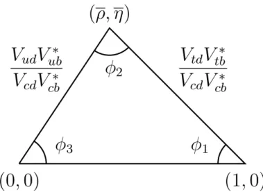
= 1. For example, the triangle generated from the first and third column of the CKM matrix (the relevant triangle for B physics at Belle) is:

V

V

+ V

V

+ V

V

= 0 (5) In a complex plane with the Wolfenstein parameters ρ and η this equation de- scribes a triangle. The angles of the triangle are interesting observables that can be extracted from the measurements of different decay channels and therefore they can nicely combine various results. The B physics triangle from equation 5 is shown in Figure 5.

Figure 5: Unitarity triangle in the (ρ, η) plane of the Wolfenstein parametrization.

This triangle is normalized by |V

V

| ≈ Aλ

and therefore the apex coordinates ( ¯ ρ, η) are given by: ¯ ¯ ρ = ρ

1 −

and ¯ η = η

1 −

. Source: [8, p. 14].

The parameters of this triangle are constrained by several decay channels, which are combined by the CKMfitter group into one single plot [23]. The 2013 plot is shown in Figure 6. Several quantities constraining the unitarity triangle are shown.

CP Violation (

CP)

CP means that the Lagrangian of the system is not invariant under a combined

application of a parity and a charge conjugation. The

CP within the SM originates

from the complex phase in the CKM matrix. In the weak mixing of neutral mesons (e.g. B

B ¯

), several CKM matrix elements are involved and a proper parametriza- tion needs to be chosen. The time evolution of the B meson system is described by a Schr¨ odinger like equation [8]:

i d

dt |B(t)i =

M − i Γ 2

|B(0)i (6)

where M and Γ are the hermitian mass and decay matrices respectively, and

|B (t)i is the ket describing the mixed state. The eigenstates of the matrix M − i

are given by [8]:

14

Figure 6: 2013 plot from CKMfitter. Source: [23]

|B

i = p|B

i + q| B ¯

i

|B

i = p|B

i − q| B ¯

i (7) where q and p are the (complex) mixing parameters. In the decay of the system there are four different possible amplitudes A:

A

= Br(B → f ) A

= Br(B → f ¯ ) A ¯

= Br( ¯ B → f ) A ¯

= Br( ¯ B → f ¯ )

(8)

where Br stands for Branching ratio. With these parameters three types of

CP

are distinguished: direct

CP in the decay, indirect

CP in the mixing and

CP in the

interference of mixing and decay [24].

15

1. Direct

CP occurs if the decay amplitude of the particle into a final state is

different to the decay amplitude of the anti particle to the anti final state, i.e.

A

6= ¯ A

or alternatively by requiring [24]:

A

A ¯

6= 1 (9)

2. Indirect

CP is characterized by the mixing parameters

q and p from equation 7. It describes that an oscillating neutral meson particle anti-particle system is more likely to oscillate to one of the both states than to the other. It occurs if [24]:

q p

6= 1 (10)

3. The third type of

CP is also called

CP in the

interference. The amplitude of a particle decaying into its final state A

is compared to the amplitude of the particle first oscillating to its anti-particle and then decaying to the final state ¯ A

. This type of

CP is characterized by [24]:

Im A

A ¯

· q p

6= 0 (11)

2.1.2 B Factories as Complementary Approach to the LHC

The B factories KEKB with the Belle experiment [19] and PEPII with the BaBar [20] experiment were able to provide many successful results that could confirm the SM in the quark flavor sector [8]. Especially the “golden channel” [5] B

→ J/ψK

was first measured with a high precision and allowed to extract the angle Φ

of the unitarity triangle. In these experiments the measurements of various decay modes allowed the extraction of many CKM matrix elements, unitarity triangle values and other interesting observables. These high precision measurements uncovered the CKM mechanism to be the dominant source of the observable

CP, which is now a

part of the SM [8].

Flavor Physics Reach

Despite the tremendous success of the B factories in confirming the SM quark flavor sector up to the GeV scale, there are still many open questions where the machines met their limits. For rare channels the available amount of data collected by Belle and BaBar is not sufficient for high precision measurements, such that the nature of these processes can not be fully understood yet. This encourages the implemen- tation of a higher luminosity B factory, which can improve the accuracy of the measurements [9].

In several decay modes there are currently little tensions between the measured values and the SM expectation with deviations of up to O(≈ 3σ). Furthermore, there were new resonances found, which are not yet declared within the SM, e.g.

the discovery of the X(3872) in 2003 [9] with the quantum numbers J

= 1

determined by LHCb in 2013 [25]. In general, higher order corrections are expected in decays, which only have a small effect relative to the dominating Leading Order (LO) process. However, with a higher precision measurement the characteristic of

16

these higher order processes could be observed. Therefore, the high precision allows to peek into the TeV scale processes which only occurs in the loop corrections [8].

Several properties of the SM need to be clarified by future experiments. The SM is only a phenomenological theory that describes the observed structure of particle physics interactions. But the SM introduces many free parameters and these have to be determined by experiments. Among these parameters are the masses of the particles, which are introduced by the Higgs mechanism and the

CP parameters.

The Higgs mass has quadratic divergent radiative corrections and therefore its mass (≈ O(125 GeV) is of the same order as the cut off scale [8]. This affirms the current expectation to observe the existence of NP processes at the TeV scale.

In the parameters of the CKM matrix a hierarchy in the measured matrix ele- ments can be observed, which cannot be explained within the SM. This hierarchy may indicate NP in a flavor symmetry at higher energy scales [8]. To leading order in the Wolfenstein approximation the CKM matrix is a unit matrix, which could indicate a generic flavor structure at high energy scales. Current measurements im- ply that such a generic flavor structure is only possible at energy scales above O(10

TeV) [21].

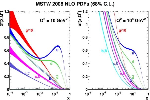
Figure 7: Parton distribution function for proton collisions at two different values of Q

. For lower Q

the valence quarks are dominating, but at higher Q

the virtual particles achieve nearly equal probability. Source: [26, p. 5].

Comparison with LHC

Especially the known CM energy is an advantage of the B factories. In an electron positron collision always the full particles interact with each other. If an event is reconstructed, also the missing momentum can be calculated, and therefore also neutrinos can be detected. In contrast, at high energy machines like the LHC, the CM energy is unknown. This is due to the different production mechanisms: in a

17

proton proton collision at the LHC not the whole protons interact with each other, but only partons within the protons interact (valence quarks, see quarks, gluons).

Each of these partons only carries an unknown fraction x of the total momentum and therefore the CM energy can only be inferred from the decay products, but is not known beforehand [8].

In Figure 7 a parton distribution function relevant for the LHC is shown for two different energy scales (Q

values) [26]. This function describes the probability to find a parton of a certain type with the momentum fraction x at the energy scale Q

. Only for lower energy scales the quark content of the proton (uud) is dominating.

At higher energy scales the probability to find see quark approaches the probability to find valence quarks and the gluons have the highest probability to be found at all.

Basically, one can differentiate the high precision and the high energy machines.

The goal of the high energy machines is the direct production of new particles by providing sufficient energy [9]. If the momentum fraction of the two interacting partons is sufficient, new resonances can be found. In the high precision experi- ments, the particles directly produced are well known. The goal is to measure the properties in the different decay channels with a high precision. By correlating the various decay modes, it is possible to identify parts of the flavor structure beyond the standard model.

Figure 8: Possible sensitivity to NP of SuperKEKB compared to the LHC. For a flavor violating NP coupling the mass of the NP particle M

vs. the NP coupling strength g

is shown. Source: [9, p. 3].

The different physical reach of LHC and SuperKEKB is shown in Figure 8. It shows the coupling strength of a NP process vs. the mass of the NP particle [9].

The line for the LHC is flat because the LHC produces particles directly via the available CM energy. The physics reach is therefore proportional to the beam en-

18

ergy. Because only fractions of the protons interact, also only a fraction of the total energy is available for new resonances. This leads to the mass reach limit of O(≈ 1 TeV) for direct production [9]. For SuperKEKB the line is diagonal because knowl- edge on new physics processes is extracted from loop corrections possibly containing NP particles. Rare flavor channels at lower energy scales can be measured with a high precision, and deviations from the SM expectation can be used to detect NP signatures [9]. Therefore, the physics reach is proportional to the coupling strength of the NP process.

19

2.2 Background in the Belle II Experiment

Background is inherently present in particle physics experiments. It refers to physics processes that cause a signal in the detector but which do not belong to the decay of the Υ(4S) particles. These background processes need to be identified as early as possible such that the signal to noise ratio in the collected data can be optimized.

The main background contribution will be beam induced [9]. Compared to Belle, a severe background occupancy can be expected due to the increased luminosity [6]. The physics properties of the beam focusing and the geometry of collider and detector allow to estimate background expectations. Starting with the experience from the Belle detector and using Monte Carlo simulations of the Belle II detector several studies on the expected background were performed in [27], [6].

Background is problematic for different parts of the detector. At first, the back- ground radiation can cause damage in the detector material itself. For this reason the Machine Detector Interface (MDI) is a crucial component to protect the detector [6]. Where possible the sensitive parts of the detector are shielded against the ex- pected background types or countermeasures are installed to avoid the background to hit the detector. The radiation that circumvents the shields hits the detector components and causes a signal there. The first evaluation of these possible back- ground signals is then performed by the trigger system. After a positive decision from the trigger system, the data collected in all the detector components is read out and recorded for a later offline analysis.

In this subsection the expected types of background and their production mecha- nisms are discussed. Special focus is set on the background that is visible within the CDC, because this detector is used as input for the z-vertex trigger task. Since sev- eral background types are correlated with the essential machine parameters, these are adressed in Subsection 2.2.1. In Subsection 2.2.2 the known types of beam in- duced background processes are shown.

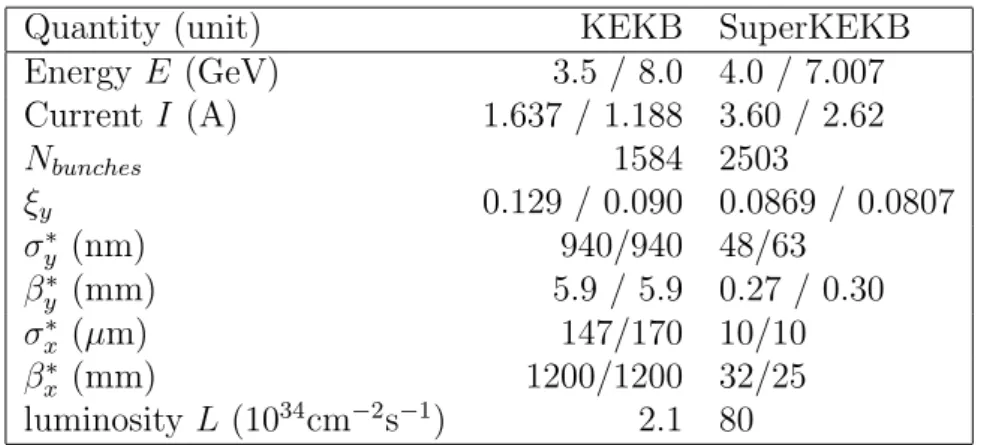
2.2.1 Machine Properties

Which background is present depends on the physical properties of the accelerator, the detector, and the focussing optics at the IP [9]. The most crucial component in the description of a particle physics experiment is its luminosity L, which relates the rate of events to the differential cross section. The target luminosity for the Belle II experiment is L = 8 · 10

cm

s

[6], [9] which is by a factor of ∼ 40 higher than in Belle. This huge increase in luminosity is achieved by the “Nano-Beam”

scheme, where the vertical beta function at the IP (β

) is heavily reduced [9]. Other important quantities are the energies of the colliding e

/ e

particles E

, the beam currents I

, and the number of bunches N

. The luminosity in SuperKEKB will be given by [9]:

L = γ

2er

I

ξ

β

R

R

| {z }

v1

(12)

where the suffix ± denotes the product of the quantity for the LER and the HER beam, γ is the Lorentz factor, e the elementary charge, r

the classical electron ra-

20

dius, I is the beam current, ξ

the vertical beam-beam parameter, β

is the vertical beta function at the IP, R

and R

are reduction factors for the luminosity and the vertical beam-beam parameter [9]. The values for the parameters in SuperKEKB compared to the values in KEKB are listed in Table 3.

Quantity (unit) KEKB SuperKEKB

Energy E (GeV) 3.5 / 8.0 4.0 / 7.007 Current I (A) 1.637 / 1.188 3.60 / 2.62

N

1584 2503

ξ

0.129 / 0.090 0.0869 / 0.0807

σ

(nm) 940/940 48/63

β

(mm) 5.9 / 5.9 0.27 / 0.30

σ

(µm) 147/170 10/10

β

(mm) 1200/1200 32/25

luminosity L (10

cm

s

) 2.1 80

Table 3: Basic SuperKEKB parameters compared to KEKB. The two values in each field correspond to LER/HER. Source: [6].

2.2.2 Beam Induced Background Types

In [27], [9] and [6] several types of beam induced background types are listed and the amount of the background types is estimated. The discussed background types are:

Beam-Gas, Touschek, Synchrotron Radiation (SR), radiative Bhabha scattering (RBB), Two Photon, and Beam Beam.

In the following the beam induced background types are shortly explained. A more detailed description can be found in [6], [27], [9]:

1. Touschek

The Touschek effect is an intra bunch Coulomb scattering process. The scat- tered particles hit the beam pipe and the magnets where they cause shower particles. The Touschek scattering rate Γ is proportional to: Γ ∝ N

· I

E

· σ

where E is the beam energy, N

is the number of bunches, I is the beam current, and σ

is the beam size [6]. Due to the E

dependence and due to the lower bunch current density in the HER, the HER contributions to the Touschek background can be ignored [27]. Because of the ”Nano-Beam”

schema the beam size at SuperKEKB is much smaller than at KEKB and therefore Touschek is a dangerous source of background. Simple extrapolations from KEKB using the new machine parameters from SuperKEKB predict the increase to be a factor of ∼ 20 [6].

2. Beam Gas

This type of background is caused by residual gas atoms in the beam pipe. The momenta of the beam particles are changed by Coulomb and bremsstrahlung scattering at the residual atoms [9]. Finally, the scattered particles hit the walls of the vacuum chamber and the magnets and cause shower particles,

21

similar to the Touschek background [6]. The amount of beam gas background is mainly dependent on the beam currents I and the vacuum pressure [9].

Latest simulations have shown that the Coulomb scattering rate with respect to KEKB is increased by a factor of ∼ 100 [6]. The reason is that the beam pipe surrounding the IP is smaller, and the maximum vertical beta function is larger than in Belle [6].

3. Synchrotron Radiation (SR)

SR consists of high energetic photons which are emitted from the beam as it is curved in the magnetic field. Its power is proportional to E

and B

, where E is the beam energy and B is the magnetic field. Because of the higher beam energy, the main source for SR is the HER. The expected energy is in the order O(1 − 10) keV. To protect the inner detectors (PXD/SVD), gold plate is installed at the inner surface of the beryllium beam pipe [6].

4. Radiative Bhabha

In the radiative Bhabha scattering, photons are emitted along the beam axis direction, such that they interact with the wall. Via the giant photo-nuclear effect, neutrons are emitted from the walls of the beampipe. These neutrons are the main background source for the outer detectors [6]. This effect is proportional to the luminosity, and therefore a factor of ∼ 40 can be expected.

5. two-photon

This type of background is very low momentum e

e

pair background which is produced via a two photon process: e

e

→ e

e

e

e

. Because of the

1

r

behaviour of the two-photon background, this type of background is only relevant for the inner parts of the detector (especially the PXD). [6]

6. Beam Beam

A beam interacts with the electric field of the other beam. The effect is that beam particles are kicked with a force that is almost proportional to their distance from the bunch-center [6].

In Table 4 the relative contributions of several background types in the Belle CDC are shown and an expected scaling factor for the CDC in Belle II is given based on the analysis in [27]. Because at the time of this study the machine parameters were not decided yet, in this analysis the machine parameters do not correspond to the anticipated machine parameters. Therefore, this analysis can only give a rough insight and should not be interpreted quantitatively.

Background type fraction in CDC expected scaling in CDC

Beam Gas HER 0.25 14

Beam Gas LER 0.4 24

Touschek 0.1 23 - 46

SR 0.24 6

Radiative Bhabha 0.01 30

Table 4: Relative contributions of the background types in Belle. Source: [27, p.

4-6].

22

Using the scale factors in Table 4 the background trend was estimated in [27].

There, a gradual increase in the beam currents is expected. The extrapolated back- ground expectation for the CDC is shown in Figure 9. The tendency in Figure 9 indicates that the most severe background contribution comes from Beam Gas scat- tering and from the Touschek effect.

Figure 9: Expectation of the background levels normalized to Belle background level found by extrapolating. Source: [27, p. 10].

To summarize, the most dangerous background contribution is the Touschek effect because of the “Nano-Beam” schema. Like the beam gas scattering it has the effect that particles from the beam hit the beam pipe somewhere, and secondary radiation or showers are caused. For the z-vertex studies this means that a significant amount of background can be expected to be the radiating beampipe. Since the beampipe roughly coincides with the z-axis of the coordinate system centered at the IP, a z-vertex trigger could be very helpful in detecting the Touschek background.

23

2.3 Background Suppression with the Z -Vertex Trigger

The main components of the trigger system and their relevance for a neural network trigger system were already reviewed in [1]. For more detailed information on the trigger see [9] and [28]. This subsection briefly presents the main features, then the improvement that could be achieved using the neural network z-vertex trigger is discussed.

The Belle II trigger system provides an online background suppression, by using detector components with a short read out time. The high requirements on the trigger system are:

“a high efficiency for hadronic events from Υ(4S) → B B ¯ and continuum pro- duction of quark pairs, a maximum average trigger rate of 30 kHz, a fixed latency of about 5 µs, a timing precision of less than 10 ns, a minimum two-event separation of 200 ns, and a trigger configuration that is flexible and robust.”[28]

Very fast procedures are necessary to meet the 5 µs latency which additionally have to operate in a pipeline to achieve the two-event separation of 200 ns.

A trigger system aims to identify features which allow to decide, whether the measured data belongs to an intended decay from the IP, or whether it is back- ground. In principle there are two different trigger strategies: either the goal is to identify physics signal, a vote from these trigger components implies that the data should be recorded for a later offline analysis; or the goal is to identify background, a vote from these trigger components implies that the data should be rejected.

The trigger components in the Belle II trigger system related to the neural net- work trigger studies are:

1. the Track Segment Finder (TSF) that prepares the CDC wire hit information for the trigger system by combining several wire hits to CDC TS.

2. the 2D and 3D trigger system that use the same input data from the TSF.

The 2D trigger provides p

and φ information and can be used as input to the neural network system. The 3D trigger is too slow to be used as input therefore it operates in parallel. Its output values are θ and z for each track found by the 2D system. The neural networks could improve this prediction using an alternative approach for the 3D reconstruction.

3. the Global Decision Logic (GDL) of the trigger system provides the final trigger decision by combining the information from the different trigger sub systems.

Although, the components are not yet implemented, the anticipated algorithms are already discussed. The output rate of the TSF is 32 ns, and the provided information consists of a hit map for the hit states of the active TS in the last 32 ns time window plus detail information for each active TS [29]. The hit map has 1 bit for each of the 2336 TS. The detail information includes 4 bit drift times [29] of the active track segments within the 32 ns window (i.e. 2 ns resolution).

But the drift times do not necessarily correspond to the central wire of the track segment, there are two options for second priority drift times which can be used if the central wire was not hit [29]. Therefore, 2 bits provide the information which wire within the TS is the reference position for the drift time. In addition, a left/right ambiguity information will be provided by the TSF by additional 2 bits (left, right,

24

no information) [29]. Additional 4 bits will be required in the drift time description to cover not only the last 32 ns but the full maximum drift time of ≈ 500 ns. In total this corresponds to 12 bits detail information for each active TS.

In order to correctly interpret the output of the TSF, the TSF algorithm needs to be further investigated and efficiency measurements are required to know how the actual input will look like. Unfortunately it is not yet implemented in the simulation software of the Belle II detector “basf2”.

A general remark on the drift times is, that the drift times from the TSF will not be the absolute drift time values in the event, because t

, the initial time of the event, is not known beforehand. Instead, the provided drift times are only relatively correct within the current time window and they have a random offset with respect to the absolute drift times. t

is itself a parameter that has to be measured within the trigger system and it will be used in the GDL to provide the final trigger decision.

In the already planned trigger system the first trigger in the CDC subtrigger is the 2D trigger, which operates in the rφ plane and uses only the axial layers of the CDC as input. It performs a variant of the Hough transformation and a conformal transformation in order to retrieve the number of tracks visible in the event. Using a fast fit mechanism for each track measured values of p

and φ are provided [28].

The next algorithm in the trigger system is the 3D trigger which performs a fast track fit algorithm using also the stereo layers of the CDC [9]. Its output is the additional 3D information for each track that was found by the 2D trigger, i.e. the track parameters θ and z.

Unfortunately, the experience with Belle indicates that the accuracy of the z- vertex prediction is a difficult task with a probably much lower resolution than desired. On the other hand, the well known position of the IP would allow a very narrow cut because all the interesting physics processes occur within a distance of

≈ 1 cm along the z-axis to the IP [1], where the 1 cm interval is a rough estimate including the boost along the z-axis and the decay width of the B mesons. In Figure 1 the plot shows the fatal situation in the Belle detector that encourages the search for novel triggering techniques.

Experiments with the MLP demonstrated demonstrated its capabilities to achieve a z-resolution of ≈ 1 cm. The evidence is given in Figure 3, where the MLP res- olution for two single track events in a small phase space element in φ and θ with different p

values turned out to achieve the required high resolution of ≈ 1 cm. If a 3σ interval is kept, a cut could be applied at ≈ 3 cm. The tremendous success of the single MLP is encouraging its use in a z-vertex prediction machine. Since the MLP sensitively depends on the previous determination of the parameters p

, φ, θ a proper pre-processing needs to be applied.

In the best case the 2D and 3D trigger systems can both be used as pre-processors for the MLP. If the accuracy is sufficient and if the latency of these methods is small enough, a specialized MLP can simply be selected using the parameters provided by these methods. To the current knowledge, the latency of the 2D trigger is small enough to be used as pre-processor. Whether the 3D trigger is fast enough has to be tested in future experiments. To the current knowledge, a solution independent of the 3D trigger is required.

25

For the case that the information of the other trigger components is not suffi- cient, in [1] a LUT approach was introduced. A pre-processing system then combines the available information of LUT and the trigger system, in order to select the opti- mal MLP. Future experiments need to investigate the optimal pre-processing system.

TSF 2D

Hough

3D TRG

LUT Bayes

Find NN

Sectors Run NN

φ, p

φ, p

, (θ)

p

, φ, θ, z

z

t Trigger System

NN Z Trigger

Figure 10: Signal flow relevant for the neural network z-vertex trigger. The 2D trigger output can be used as input to the neural network system, but latency does not allow to use the 3D trigger information. Source: [1, p. 13]

The currently anticipated signal flow is shown in Figure 10. The output of the TSF are hits which are used as input to the 2D and 3D trigger. The hits are also used as input to the LUT approach. By combining the information of the 2D trigger and the LUT, a prediction of the track parameters p

, φ, θ is provided. Based on this prediction a proper MLP weight set that is trained to this special p

, φ, θ sector can be loaded. After the weight loading, the MLP can process the TSF input and provide the desired z-vertex value.

26