Real-Time Adaptive Image Compression

(1)

Real-Time Adaptive Image Compression

Oren Rippel^{* 1} Lubomir Bourdev^{* 1}

Abstract

We present a machine learning-based approach to lossy image compression which outperforms all existing codecs, while running in real-time.

Our algorithm typically produces files 2.5 times smaller than JPEG and JPEG 2000, 2 times smaller than WebP, and 1.7 times smaller than BPG on datasets of generic images across all quality levels. At the same time, our codec is designed to be lightweight and deployable: for example, it can encode or decode the Kodak dataset in around 10ms per image on GPU.

Our architecture is an autoencoder featuring pyramidal analysis, an adaptive coding module, and regularization of the expected codelength.

We also supplement our approach with adversarial training specialized towards use in a compression setting: this enables us to produce visually pleasing reconstructions for very low bitrates.

1. Introduction

Streaming of digital media makes 70% of internet traffic, and is projected to reach 80% by 2020 (CIS,2015). How- ever, it has been challenging for existing commercial compression algorithms to adapt to the growing demand and the changing landscape of requirements and applications.

While digital media are transmitted in a wide variety of settings, the available codecs are “one-size-fits-all”: they are hard-coded, and cannot be customized to particular use cases beyond high-level hyperparameter tuning.

In the last few years, deep learning has revolutionized many tasks such as machine translation, speech recognition, face recognition, and photo-realistic image generation. Even though the world of compression seems a natural domain for machine learning approaches, it has not yet benefited from these advancements, for two main reasons. First,

*Equal contribution ¹WaveOne Inc., Mountain View, CA, USA. Correspondence to: Oren Rippel <oren@wave.one>, Lubomir Bourdev<lubomir@wave.one>.

our deep learning primitives, in their raw forms, are not well-suited to construct representations sufficiently compact. Recently, there have been a number of important efforts byToderici et al.(2015; 2016), Theis et al. (2016), Ball´e et al.(2016), andJohnston et al.(2017) towards al- leviating this: see Section 2.2. Second, it is difficult to develop a deep learning compression approach sufficiently efficient for deployment in environments constrained by computation power, memory footprint and battery life.

In this work, we present progress on both performance and computational feasibility of ML-based image compression.

Our algorithm outperforms all existing image compression approaches, both traditional and ML-based: it typically produces files 2.5 times smaller than JPEG and JPEG 2000 (JP2), 2 times smaller than WebP, and 1.7 times smaller than BPG on the Kodak PhotoCD and RAISE-1k512×768 datasets across all of quality levels. At the same time, we designed our approach to be lightweight and efficiently deployable. On a GTX 980 Ti GPU, it takes around 9ms to encode and 10ms to decode an image from these datasets:

for JPEG, encode/decode times are 18ms/12ms, for JP2 350ms/80ms and for WebP 70ms/80ms. Results for a representative quality level are presented in Table1.

To our knowledge, this is the first ML-based approach to surpass all commercial image compression techniques, and moreover run in real-time.

We additionally supplement our algorithm with adversarial training specialized towards use in a compression setting.

This enables us to produce convincing reconstructions for very low bitrates.

Codec

RGB file size (kb)

YCbCr file size (kb)

Encode time (ms)

Decode time (ms) Ours 21.4 (100%) 17.4 (100%) 8.6^∗ 9.9^∗

JPEG 65.3 (304%) 43.6 (250%) 18.6 13.0

JP2 54.4 (254%) 43.8 (252%) 367.4 80.4

WebP 49.7 (232%) 37.6 (216%) 67.0 83.7

Table 1.Performance of different codecs on the RAISE-1k512×

768dataset for a representative MS-SSIM value of 0.98 in both RGB and YCbCr color spaces. Comprehensive results can be found in Section5.^∗We emphasize our codec was run on GPU.

arXiv:1705.05823v1 [stat.ML] 16 May 2017

(2)

JPEG

0.0826 BPP (7.5% bigger)

JPEG 2000 0.0778 BPP

WebP

0.0945 BPP (23% bigger)

Ours 0.0768 BPP

JPEG

0.111 BPP (10% bigger)

JPEG 2000 0.102 BPP

WebP

0.168 BPP (66% bigger)

Ours 0.101 BPP Figure 1.Examples of reconstructions by different codecs for very low bits per pixel (BPP) values. The uncompressed size is 24 BPP, so the examples represent compression by around 250 times. We reduce the bitrates of other codecs by their header lengths for fair comparison. For each codec, we search over bitrates and present the reconstruction for the smallest BPP above ours. WebP and JPEG were not able to produce reconstructions for such low BPP: the reconstructions presented are for the smallest bitrate they offer. More examples can be found in the appendix.

2. Background & Related Work

2.1. Traditional compression techniques

Compression, in general, is very closely related to pattern recognition. If we are able to discover structure in our input, we can eliminate this redundancy to represent it more succinctly. In traditional codecs such as JPEG and JP2, this is achieved via a pipeline which roughly breaks down into 3 modules: transformation, quantization, and encoding (Wallace(1992) andRabbani & Joshi(2002) provide great overviews of the JPEG standards).

In traditional codecs, since all components are hard-coded, they are heavily engineered to fit together. For example, the coding scheme is custom-tailored to match the distribution of the outputs of the preceding transformation. JPEG, for instance, employs 8×8 block DCT transforms, followed by run-length encoding which exploits the sparsity pattern of the resultant frequency coefficients. JP2 employs an adaptive arithmetic coder to capture the distribution of coefficient magnitudes produced by the preceding multiresolution wavelet transform.

However, despite the careful construction and assembly of

these pipelines, there still remains significant room for im- provement of compression efficiency. For example, the transformation is fixed in place irrespective of the distribution of the inputs, and is not adapted to their statistics in any way. In addition, hard-coded approaches often com- partmentalize the loss of information within the quantization step. As such, the transformation module is chosen to be bijective: however, this limits the ability to reduce redundancy prior to coding. Moreover, the encode-decode pipeline cannot be optimized for a particular metric beyond manual tweaking: even if we had the perfect metric for image quality assessment, traditional approaches cannot di- rectly optimize their reconstructions for it.

2.2. ML-based lossy image compression

In approaches based on machine learning, structure is au- tomaticallydiscovered, rather than manually engineered.

One of the first such efforts byBottou et al. (1998), for example, introduced the DjVu format for document image compression, which employs techniques such as segmen- tation and K-means clustering separate foreground from background, and analyze the document’s contents.

(3)

Target Reconstruction Bitstream

Quantization Coding

Reconstruction loss

Discriminator loss Adaptive

codelength regularization

Decoding Synthesis from features Feature

extraction

Figure 2.Our overall model architecture. The feature extractor, described in Section3.1, discovers structure and reduces redundancy via the pyramidal decomposition and interscale alignment modules. The lossless coding scheme, described in Section3.2, further compresses the quantized tensor via bitplane decomposition and adaptive arithmetic coding. The adaptive codelength regularization then modulates the expected code length to a prescribed target bitrate. Distortions between the target and its reconstruction are penalized by the reconstruction loss. The discriminator loss, described in Section4, encourages visually pleasing reconstructions by penalizing discrepancies between their distributions and the targets’.

At a high level, one natural approach to implement the encoder-decoder image compression pipeline is to use an autoencoder to map the target through a bitrate bottleneck, and train the model to minimize a loss function penalizing it from its reconstruction. This requires carefully construct- ing a feature extractor and synthesizer for the encoder and decoder, selecting an appropriate objective, and possibly introducing a coding scheme to further compress the fixed- size representation to attain variable-length codes.

Many of the existing ML-based image compression approaches (including ours) follow this general strategy.

Toderici et al. (2015;2016) explored various transforma- tions for binary feature extraction based on different types of recurrent neural networks; the binary representations were then entropy-coded. Johnston et al.(2017) enabled another considerable leap in performance by introducing a loss weighted with SSIM (Wang et al.,2004), and spatially- adaptive bit allocation. Theis et al.(2016) andBall´e et al.

(2016) quantize rather than binarize, and propose strategies to approximate the entropy of the quantized representation:

this provides them with a proxy to penalize it. Finally, Pied Piper has recently claimed to employ ML techniques in its Middle-Out algorithm (Judge et al.,2016), although their nature is shrouded in mystery.

2.3. Generative Adversarial Networks

One of the most exciting innovations in machine learning in the last few years is the idea of Generative Adversarial Networks (GANs) (Goodfellow et al.,2014). The idea is to construct a generatornetworkGΦ(·)whose goal is to synthesize outputs according to a target distribution p_true, and a discriminatornetworkDΘ(·)whose goal is to dis- tinguish between examples sampled from the ground truth distribution, and ones produced by the generator. This can be expressed concretely in terms of the minimax problem:

min

Φ max

Θ E^x∼ptruelogDΘ(x) +E^z∼pzlog [1−DΘ(GΦ(z))] . This idea has enabled significant progress in photo-realistic image generation (Denton et al., 2015; Radford et al., 2015;Salimans et al.,2016), single-image super-resolution

(Ledig et al.,2016), image-to-image conditional translation (Isola et al.,2016), and various other important problems.

The adversarial training framework is particularly relevant to the compression world. In traditional codecs, distortions often take the form of blurriness, pixelation, and so on.

These artifacts are unappealing, but are increasingly no- ticeable as the bitrate is lowered. We propose a multiscale adversarial training model to encourage reconstructions to match the statistics of their ground truth counterparts, resulting in sharp and visually pleasing results even for very low bitrates. As far as we know, we are the first to propose using GANs for image compression.

3. Model

Our model architecture is shown in Figure 2, and comprises a number of components which we briefly outline below. In this section, we limit our focus to operations per- formed by the encoder: since the decoder simply performs the counterpart inverse operations, we only address excep- tions which require particular attention.

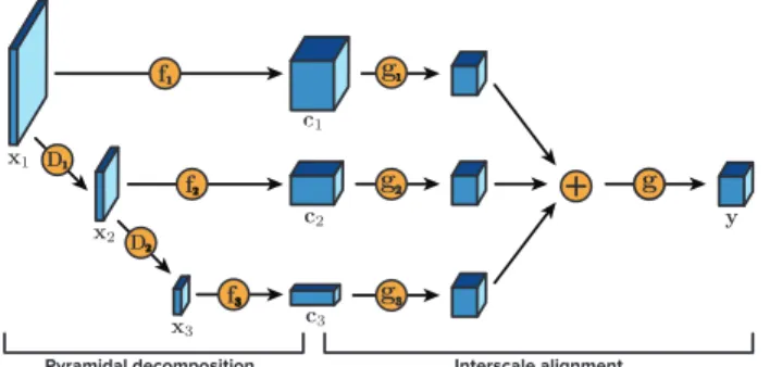
Feature extraction. Images feature a number of different types of structure: across input channels, within individual scales, and across scales. We design our feature extraction architecture to recognize these. It consists of a pyramidal decomposition which analyzes individual scales, followed by an interscale alignment procedure which exploits structure shared across scales.

Code computation and regularization. This module is responsible for further compressing the extracted features.

It quantizes the features, and encodes them via an adaptive arithmetic coding scheme applied on their binary expan- sions. An adaptive codelength regularization is introduced to penalize the entropy of the features, which the coding scheme exploits to achieve better compression.

Discriminator loss. We employ adversarial training to pursue realistic reconstructions. We dedicate Section4 to describing our GAN formulation.

(4)

3.1. Feature extraction

3.1.1. PYRAMIDAL DECOMPOSITION

Our pyramidal decomposition encoder is loosely inspired by the use of wavelets for multiresolution analysis, in which an input is analyzed recursively via feature extraction and downsampling operators (Mallat, 1989). The JPEG 2000 standard, for example, employs discrete wavelet transforms with the Daubechies 9/7 kernels (An- tonini et al.,1992;Rabbani & Joshi,2002). This transform is in fact a linear operator, which can be entirely expressed via compositions of convolutions with only twohard-coded and separable9×9filters applied irrespective of scale, and independently for each channel.

The idea of a pyramidal decomposition has been employed in machine learning: for instance, Mathieu et al.(2015) uses a pyramidal composition for next frame prediction, andDenton et al.(2015) uses it for image generation. The spectral representations of CNN activations have also been investigated by Rippel et al. (2015) to enable processing across a spectrum of scales, but this approach does not enable FIR processing as does wavelet analysis.

We generalize the wavelet decomposition idea to learn op- timal, nonlinear extractors individually for each scale. Let us assume an input x to the model, and a total of M scales. We perform recursive analysis: let us denote xm

as the input to scalem; we set the input to the first scale x₁ = x as the input to the model. For each scale m, we perform two operations: first, we extract coefficients c_m = f_m(x_m) ∈ R^C^m^×H^m^×W^m via some parametrized function f_m(·) for output channels C_m, height H_m and widthW_m. Second, we compute the input to the next scale asxm+1=Dm(xm)whereDm(·)is some downsampling operator (either fixed or learned).

Our pyramidal decomposition architecture is illustrated in Figure 3. In practice, we extract across a total of M =

Pyramidal decomposition Interscale alignment

Figure 3.The coefficient extraction pipeline, illustrated for 3 scales. The pyramidal decomposition module discovers structure within individual scales. The extracted coefficient maps are then aligned to discover joint structure across the different scales.

6 scales. The feature extractors for the individual scales are composed of a sequence of convolutions with kernels 3×3or1×1and ReLUs with a leak of0.2. We learn all downsamplers as4×4convolutions with a stride of 2.

3.1.2. INTERSCALE ALIGNMENT

Interscale alignment is designed to leverage information shared across different scales — a benefit not offered by the classic wavelet analysis. It takes in as input the set of coefficients extracted from the different scales{c_m}^M_m=1⊂ R^C^m^×H^m^×W^m, and produces a single tensor of a target output dimensionalityC×H×W.

To do this, we first map each input tensor cm to the target dimensionality via some parametrized functiong_m(·).

This involves ensuring that this function spatially resam- plescmto the appropriate output map sizeH×W, and outputs the appropriate number of channelsC. We then sum g_m(cm), m = 1, . . . , M, and apply another parametrized non-linear transformationg(·)for joint processing.

The interscale alignment module can be seen in Figure3.

We denote its output as y. In practice, we choose each g_m(·)as a convolution or a deconvolution with an appropriate stride to produce the target spatial map sizeH×W; see Section5.1for a more detailed discussion. We choose g(·)simply as a sequence of3×3convolutions.

3.2. Code computation and regularization

Given the extracted tensory ∈R^C×H×W, we proceed to quantize it and encode it. This pipeline involves a number of components which we overview here and describe in detail throughout this section.

Quantization. The tensor y is quantized to bit preci- sionB:

yˆ :=QUANTIZE_B(y).

Bitplane decomposition. The quantized tensor yˆ is transformed into a binary tensor suitable for encoding via a lossless bitplane decomposition:

b:=BITPLANEDECOMPOSE_B(ˆy)∈ {0,1}^B×C×H×W . Adaptive arithmetic coding. The adaptive arithmetic coder (AAC) is trained to leverage the structure remaining in the data. It encodesbinto its final variable-length binary sequencesof length`(s):

s:=AACENCODE(b)∈ {0,1}^`(s).

Adaptive codelength regularization. The adaptive codelength regularization (ACR) modulates the distribution of the quantized representationyˆ to achieve a target

(5)

expected bit count across inputs:

Ex[`(s)] −→ `target.

3.2.1. QUANTIZATION

Given a desired precision ofBbits, we quantize our feature tensoryinto2^Bequal-sized bins as

ˆ

ychw:=QUANTIZE_B(ychw) = 1 2^B−1

2^B−1ychw . For the special caseB= 1, this reduces exactly to a binary quantization scheme. While some ML-based approaches to compression employ such thresholding, we found better performance with the smoother quantization described. We quantize withB= 6for all models in this paper.

3.2.2. BITPLANE DECOMPOSITION

We decomposeyˆinto bitplanes. This transformation maps each valueyˆchwinto its binary expansion ofBbits. Hence, each of the C spatial mapsyˆ_c ∈ R^H×W of yˆ expands intoBbinarybitplanes. We illustrate this transformation in Figure4, and denote its output asb∈ {0,1}^B×C×H×W. This transformation is lossless.

As described in Section3.2.3, this decomposition will enable our entropy coder to exploit structure in the distribution of the activations inyto achieve a compact representation. In Section3.2.4, we introduce a strategy to encourage such exploitable structure to be featured.

3.2.3. ADAPTIVE ARITHMETIC CODING

The output b of the bitplane decomposition is a binary tensor, which contains significant structure: for example, higher bitplanes are sparser, and spatially neighboring bits often have the same value (in Section3.2.4we propose a technique to guarantee presence of these properties). We exploit this low entropy by lossless compression via adaptive arithmetic coding.

Namely, we associate each bit location inbwith acontext, which comprises a set of features indicative of the bit value.

These are based on the position of the bit as well as the values of neighboring bits. We train a classifier to predict the value of each bit from its context features, and then use these probabilities to compressbvia arithmetic coding.

During decoding, we decompress the code by performing the inverse operation. Namely, we interleave between com- puting the context of a particular bit using the values of previously decoded bits, and using this context to retrieve the activation probability of the bit and decode it. We note that this constrains the context of each bit to only include features composed of bits already decoded.

3.2.4. ADAPTIVE CODELENGTH REGULARIZATION

One problem with classic autoencoder architectures is that their bottleneck has fixed capacity. The bottleneck may be too small to represent complex patterns well, which affects quality, and it may be too large for simple patterns, which results in inefficient compression. What we need is a model capable of generating long representations for complex patterns and short for simple ones, while maintaining an expected codelength target over large number of examples.

To achieve this, the AAC is necessary, but not sufficient.

We extend the architecture by increasing the dimensionality of b— but at the same time controlling its information content, thereby resulting in shorter compressed code s = AACENCODE(b) ∈ {0,1}. Specifically, we introduce the adaptive codelength regularization (ACR), which enables us to regulate the expected codelengthEx[`(s)]to a target value `_target. This penalty is designed to encourage structure exactly where the AAC is able to exploit it.

Namely, we regularize our quantized tensoryˆwith P(ˆy) = αt

CHW X

chw

n

log₂|ˆy_chw|

+ X

(x,y)∈S

log₂

ˆychw−yˆc(h−y)(w−x)

o ,

for iteration t and difference index set S = {(0,1),(1,0),(1,1),(−1,1)}. The first term penalizes the magnitude of each tensor element, and the second penalizes deviations between spatial neighbors. These enable better prediction by the AAC.

As we train our model, we continuously modulate the scalar coefficientαtto pursue our target codelength. We do this via a feedback loop. We use the AAC to monitor the mean number of effective bits. If it is too high, we in- creaseαt; if too low, we decrease it. In practice, the model reaches an equilibrium in a few hundred iterations, and is able to maintain it throughout training.

Hence, we get a knob to tune: the ratio of total bits, namely the BCHW bits available in b, to the target number of effective bits`target. This allows exploring the trade-off of increasing the number of channels or spatial map size of

Figure 4.Each of theCspatial mapsyˆ_c ∈ R^H×W ofyˆis de- composed intoBbitplanes as each elementyˆchwis expressed in its binary expansion. Each set of bitplanes is then fed to the adaptive arithmetic coder for variable-length encoding. The adaptive codelength regularization enables more compact codes for higher bitplanes by encouraging them to feature higher sparsity.

(6)

WaveOne JPEG JPEG 2000 WebP BPG

RGB

0.0 0.5 1.0 1.5 2.0

Bits per pixel 0.90

0.92 0.94 0.96 0.98 1.00

MS-SSIM

0.95 0.96 0.97 0.98 0.99

MS-SSIM 100%

150%

200%

250%

300%

Relative compressed sizes

YCbC r

0.0 0.5 1.0 1.5 2.0

Bits per pixel 0.90

0.92 0.94 0.96 0.98 1.00

MS-SSIM

0.965 0.970 0.975 0.980 0.985 0.990 0.995 MS-SSIM

100%

150%

200%

250%

Relative compressed sizes

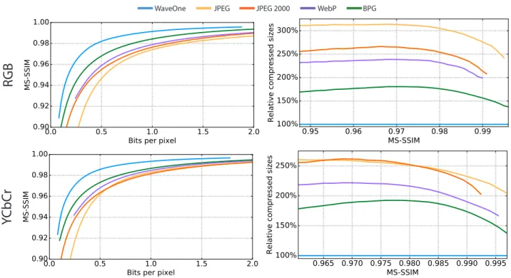
Figure 5.Compression results for the RAISE-1k512×768dataset, measured in the RGB domain (top row) and YCbCr domain (bottom row). We compare against commercial codecs JPEG, JPEG 2000, WebP and BPG⁵(4:2:0 for YCbCr and 4:4:4 for RGB). The plots on the left present average reconstruction quality, as function of the number of bits per pixel fixed for each image. The plots on the right show average compressed file sizes relative to ours for different target MS-SSIM values for each image. In Section5.2we discuss the curve generation procedures in detail.

bat the cost of increasing sparsity. We find that a total- to-target ratio ofBCHW/`_target= 4works well across all architectures we have explored.

4. Realistic Reconstructions via Multiscale Adversarial Training

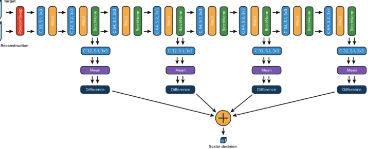
4.1. Discriminator design

In our compression approach, we take the generator as the encoder-decoder pipeline, to which we append a discriminator — albeit with a few key differences from existing GAN formulations.

In many GAN approaches featuring both a reconstruction and a discrimination loss, the target and the reconstruction are treated independently: each is separately assigned a la- bel indicating whether it is real or fake. In our formulation, we consider the target and its reconstruction jointly as a single example: we compare the two by askingwhich of the two images is the real one.

To do this, we first swap between the target and reconstruction in each input pair to the discriminator with uni- form probability. Following the random swap, we propagate each set of examples through the network. How- ever, instead of producing an output for classification at the

very last layer of the pipeline, we accumulate scalar outputs along branches constructed along it at different depths. We average these to attain the final value provided to the termi- nal sigmoid function. This multiscale architecture allows aggregating information across different scales, and is mo- tivated by the observation that undesirable artifacts vary as function of the scale in which they are exhibited. For example, high-frequency artifacts such as noise and blurriness are discovered by earlier scales, whereas more abstract discrepancies are found in deeper scales.

We apply our discriminator DΘ on the aggregate sum across scales, and proceed to formulate our objectives as described in Section 2.3. The complete discriminator architecture is illustrated in Figure10.

4.2. Adversarial training

Training a GAN system can be tricky due to optimization instability. In our case, we were able to address this by de- signing a training scheme adaptive in two ways. First, the reconstructor is trained by both the confusion signal gradient as well as the reconstruction loss gradient: we balance the two as function of their gradient magnitudes. Second, at any point during training, we either train the discriminator or propagate confusion signal through the reconstructor, as function of the prediction accuracy of the discriminator.

(7)

WaveOne JPEG JPEG 2000 WebP BPG Ballé et al. Toderici et al. Theis et al. Johnston et al.

RGB

0.0 0.5 1.0 1.5 2.0

Bits per pixel 0.90

0.92 0.94 0.96 0.98 1.00

MS-SSIM

0.94 0.95 0.96 0.97 0.98 0.99 MS-SSIM

100%

150%

200%

250%

300%

Relative compressed sizes

YCbC r

0.0 0.5 1.0 1.5 2.0

Bits per pixel 0.90

0.92 0.94 0.96 0.98 1.00

MS-SSIM

0.95 0.96 0.97 0.98 0.99

MS-SSIM 100%

150%

200%

250%

300%

Relative compressed sizes

Figure 6.Performance on the Kodak PhotoCD dataset measured in the RGB domain (top row) and YCbCr domain (bottom row). We compare against commercial codecs JPEG, JPEG 2000, WebP and BPG⁵(4:2:0 for YCbCr and 4:4:4 for RGB), as well as recent ML- based compression work byToderici et al.(2016)²,Theis et al.(2016)³,Ball´e et al.(2016)⁴, andJohnston et al.(2017)³in all settings where results exist. The plots on the left present average reconstruction quality, as function of the number of bits per pixel fixed for each image. The plots on the right show average compressed file sizes relative to ours for different target MS-SSIM values for each image.

More concretely, given lower and upper accuracy bounds L, U ∈[0,1]and discriminator accuracya(DΘ), we apply the following procedure:

• If a < L: freeze propagation of confusion signal through the reconstructor, and train the discriminator.

• IfL≤a < U: alternate between propagating confusion signal and training the disciminator.

• IfU ≤a: propagate confusion signal through the reconstructor, and freeze the discriminator.

In practice we usedL= 0.8, U = 0.95. We compute the accuracyaas a running average over mini-batches with a momentum of0.8.

5. Results

5.1. Experimental setup

Similarity metric. We trained and tested all models on the Multi-Scale Structural Similarity Index Metric (MS- SSIM) (Wang et al.,2003). This metric has been specifically designed to match the human visual system, and has been established to be significantly more representative than losses in the`_pfamily and variants such as PSNR.

Color space. Since the human visual system is much more sensitive to variations in brightness than color, most codecs represent colors in the YCbCr color space to de- vote more bandwidth towards encoding luma rather than chroma. In quantifying image similarity, then, it is common to assign the Y, Cb, Cr components weights 6/8,1/8,1/8. While many ML-based compression pa- pers evaluate similarity in the RGB space with equal color weights, this does not allow fair comparison with standard codecs such as JPEG, JPEG 2000 and WebP, since they have not been designed to perform optimally in this domain. In this work, we provide comparisons with both traditional and ML-based codecs, and present results in both the RGB domain with equal color weights, as well as in YCbCr with weights as above.

Reported performance metrics. We present both compression performance of our algorithm, but also its runtime.

While the requirement of running the approach in real-time severely constrains the capacity of the model, it must be met to enable feasible deployment in real-life applications.

Training and deployment procedure. We trained and tested all models on a GeForce GTX 980 Ti GPU and a custom codebase. We trained all models on128×128patches sampled at random from the Yahoo Flickr Creative Com-

(8)

mons 100 Million dataset (Thomee et al.,2016).

We optimized all models with Adam (Kingma & Ba,2014).

We used an initial learning rate of3×10⁻⁴, and reduced it twice by a factor of 5 during training. We chose a batch size of 16 and trained each model for a total of 400,000 iterations. We initialized the ACR coefficient asα0 = 1.

During runtime we deployed the model on arbitrarily-sized images in a fully-convolutional way. To attain the rate- distortion (RD)curves presented in Section5.2, we trained models for a range of target bitrates`target.

5.2. Performance

We present several types of results:

1. Average MS-SSIM as function of the BPP fixed for each image, found in Figures5and6, and Table1.

2. Average compressed file sizes relative to ours as function of the MS-SSIM fixed for each image, found in Figures5and6, and Table1.

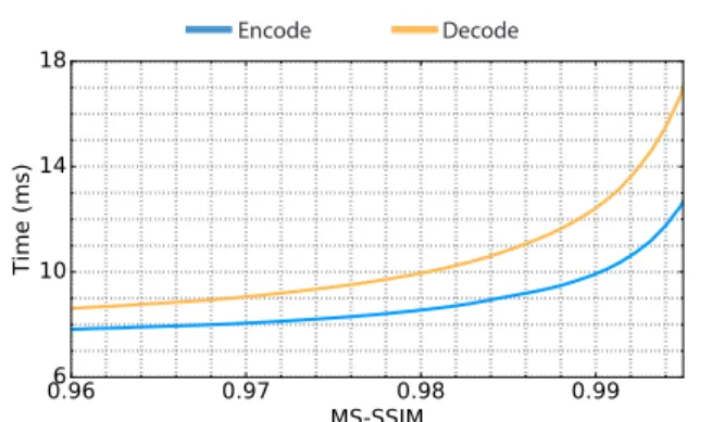
3. Encode and decode timings as function of MS-SSIM, found in Figure7, in the appendix, and Table1.

4. Visual examples of reconstructions of different compression approaches for the same BPP, found in Fig- ure1and in the appendix.

Test sets. To enable comparison with other approaches, we first present performance on the Kodak PhotoCD dataset¹. While the Kodak dataset is very popular for testing compression performance, it contains only 24 images, and hence is susceptible to overfitting and does not necessarily fully capture broader statistics of natural images. As such, we additionally present performance on the RAISE-1k dataset (Dang-Nguyen et al.,2015) which contains 1,000 raw images. We resized each image to size 512×768(backwards if vertical): we intend to release our preparation code to enable reproduction of the dataset used.

We remark it is important to use a dataset of raw, rather than previously compressed, images for codec evaluation.

1The Kodak PhotoCD dataset can be found at http://

r0k.us/graphics/kodak.

2The results of Toderici et al. (2016) on the Ko- dak RGB dataset are available at http://github.com/

tensorflow/models/tree/master/compression.

3We have no access to reconstructions byTheis et al.(2016) andJohnston et al.(2017), so we carefully transcribed their results, only available in RGB, from the graphs in their paper.

4Reconstructions byBall´e et al.(2016) of images in the Ko- dak dataset can be found at http://www.cns.nyu.edu/

˜lcv/iclr2017/for both RGB and YCbCr and across a spectrum of BPPs. We use these to compute RD curves by the procedure described in this section.

5An implementation of the BPG codec is available athttp:

//bellard.org/bpg.

Encode Decode

0.96 0.97 0.98 0.99

MS-SSIM 6

10 14 18

Time (ms)

Figure 7.Average times to encode and decode images from the RAISE-1k512×768dataset using our approach.

Compressing an image introduces artifacts with a bias particular to the codec used, which results in a more favorable RD curve if it compressedagainwith the same codec. See Figure9for a plot demonstrating this effect.

Codecs. We compare against commercial compression techniques JPEG, JPEG 2000, WebP, as well as recent ML- based compression work byToderici et al.(2016)²,Theis et al. (2016)³, Ball´e et al. (2016)⁴, and Johnston et al.

(2017)³ in all settings in which results are available. We also compare to BPG⁵(4:2:0 and 4:4:4) which, while not widely used, surpassed all other codecs in the past. We use the best-performing configuration we can find of JPEG, JPEG 2000, WebP, and BPG, and reduce their bitrates by their respective header lengths for fair comparison.

Performance evaluation. For each image in each test set, each compression approach, each color space, and for the selection of available compression rates, we recorded (1) the BPP, (2) the MS-SSIM (with components weighted appropriately for the color space), and (3) the computation times for encoding and decoding.

It is important to take great care in the design of the performance evaluation procedure. Each image has a separate RD curve computed from all available compression rates for a given codec: asBall´e et al.(2016) discusses in detail, different summaries of these RD curves lead to disparate results. In our evaluations, to compute a given curve, we sweep across values of the independent variable (such as bitrate). We interpolate each individual RD curve at this independent variable value, and average all the results. To en- sure accurate interpolation, we sample densely across rates for each codec.

Acknowledgements We are grateful to Trevor Darrell, Sven Strohband, Michael Gelbart, Robert Nishihara, Al- bert Azout, and Vinod Khosla for meaningful discussions and input.

(9)

References

White paper: Cisco vni forecast and methodology, 2015- 2020. 2015.

Antonini, Marc, Barlaud, Michel, Mathieu, Pierre, and Daubechies, Ingrid. Image coding using wavelet transform.IEEE Trans. Image Processing, 1992.

Ball´e, Johannes, Laparra, Valero, and Simoncelli, Eero P.

End-to-end optimized image compression. preprint, 2016.

Bottou, L´eon, Haffner, Patrick, Howard, Paul G, Simard, Patrice, Bengio, Yoshua, and LeCun, Yann. High quality document image compression with djvu. 1998.

Dang-Nguyen, Duc-Tien, Pasquini, Cecilia, Conotter, Valentina, and Boato, Giulia. Raise: a raw images dataset for digital image forensics. InProceedings of the 6th ACM Multimedia Systems Conference, pp. 219–224.

ACM, 2015.

Denton, Emily L, Chintala, Soumith, Fergus, Rob, et al.

Deep generative image models using a laplacian pyramid of adversarial networks. InNIPS, pp. 1486–1494, 2015.

Goodfellow, Ian, Pouget-Abadie, Jean, Mirza, Mehdi, Xu, Bing, Warde-Farley, David, Ozair, Sherjil, Courville, Aaron, and Bengio, Yoshua. Generative adversarial nets.

InNIPS, pp. 2672–2680, 2014.

Isola, Phillip, Zhu, Jun-Yan, Zhou, Tinghui, and Efros, Alexei A. Image-to-image translation with conditional adversarial networks. arXiv preprint arXiv:1611.07004, 2016.

Johnston, Nick, Vincent, Damien, Minnen, David, Cov- ell, Michele, Singh, Saurabh, Chinen, Troy, Hwang, Sung Jin, Shor, Joel, and Toderici, George. Improved lossy image compression with priming and spatially adaptive bit rates for recurrent networks. arXiv preprint arXiv:1703.10114, 2017.

Judge, Mike, Altschuler, John, and Krinsky, Dave. Silicon valley (tv series). 2016.

Kingma, Diederik and Ba, Jimmy. Adam: A method for stochastic optimization. arXiv preprint arXiv:1412.6980, 2014.

Ledig, Christian, Theis, Lucas, Husz´ar, Ferenc, Caballero, Jose, Cunningham, Andrew, Acosta, Alejandro, Aitken, Andrew, Tejani, Alykhan, Totz, Johannes, Wang, Ze- han, et al. Photo-realistic single image super-resolution using a generative adversarial network. arXiv preprint arXiv:1609.04802, 2016.

Mallat, S. G. A theory for multiresolution signal decomposition: The wavelet representation. IEEE Trans. Pattern Anal. Mach. Intell., 11(7):674–693, July 1989.

Mathieu, Michael, Couprie, Camille, and LeCun, Yann.

Deep multi-scale video prediction beyond mean square error.arXiv preprint arXiv:1511.05440, 2015.

Rabbani, Majid and Joshi, Rajan. An overview of the jpeg 2000 still image compression standard. Signal processing: Image communication, 17(1):3–48, 2002.

Radford, Alec, Metz, Luke, and Chintala, Soumith. Un- supervised representation learning with deep convolutional generative adversarial networks. arXiv preprint arXiv:1511.06434, 2015.

Rippel, Oren, Snoek, Jasper, and Adams, Ryan P. Spec- tral representations for convolutional neural networks. In Advances in Neural Information Processing Systems, pp.

2449–2457, 2015.

Salimans, Tim, Goodfellow, Ian, Zaremba, Wojciech, Che- ung, Vicki, Radford, Alec, and Chen, Xi. Improved techniques for training gans. InNIPS, pp. 2226–2234, 2016.

Theis, Lucas, Shi, Wenzhe, Cunningham, Andrew, and Huszar, Ferenc. Lossy image compression with com- pressive autoencoders.preprint, 2016.

Thomee, Bart, Shamma, David A, Friedland, Gerald, Elizalde, Benjamin, Ni, Karl, Poland, Douglas, Borth, Damian, and Li, Li-Jia. Yfcc100m: The new data in multimedia research. Communications of the ACM, 2016.

Toderici, George, O’Malley, Sean M, Hwang, Sung Jin, Vincent, Damien, Minnen, David, Baluja, Shumeet, Covell, Michele, and Sukthankar, Rahul. Variable rate image compression with recurrent neural networks.

arXiv preprint arXiv:1511.06085, 2015.

Toderici, George, Vincent, Damien, Johnston, Nick, Hwang, Sung Jin, Minnen, David, Shor, Joel, and Covell, Michele. Full resolution image compression with recurrent neural networks. arXiv preprint arXiv:1608.05148, 2016.

Wallace, Gregory K. The jpeg still picture compression standard. IEEE transactions on consumer electronics, 38(1):xviii–xxxiv, 1992.

Wang, Zhou, Simoncelli, Eero P, and Bovik, Alan C. Mul- tiscale structural similarity for image quality assessment.

InSignals, Systems and Computers, 2004., volume 2, pp.

1398–1402. Ieee, 2003.

Wang, Zhou, Bovik, Alan C, Sheikh, Hamid R, and Si- moncelli, Eero P. Image quality assessment: from error visibility to structural similarity. IEEE transactions on image processing, 13(4):600–612, 2004.

(10)

Real-Time Adaptive Image Compression: Supplementary Material

WaveOne JPEG JPEG 2000 WebP BPG

0.96 0.97 0.98 0.99 MS-SSIM

5 10 20 40 80 160 320

Time (ms)

(a) Encode times.

0.96 0.97 0.98 0.99 MS-SSIM

5 10 20 40 120 80

Time (ms)

(b) Decode times.

Figure 8.Average times to encode and decode images from the RAISE-1k512×768dataset. Note our codec was run on GPU.

0.5 1.0 1.5 2.0 2.5 3.0

Bits per pixel 0.960

0.965 0.970 0.975 0.980 0.985 0.990 0.995 1.000

MS-SSIM

Quality 30

Quality 40 Quality 50 Quality 60 Quality 70 Quality 80 Quality 90 Uncompressed

Figure 9.We used JPEG to compress the Kodak dataset at various quality levels. For each, we then use JPEG to recompress the images, and plot the resultant rate-distortion curve. It is evident that the more an image has been previously compressed with JPEG, the better JPEG is able to then recompress it.

(11)

ReLU BatchNorm

Mean

Difference

C 32, S 2, 3x3

Difference Difference Difference

Mean Mean Mean

ReLU BatchNorm

C 64, S 1, 3x3 ReLU BatchNormC 64, S 2, 3x3 ReLU BatchNormC 64, S 1, 3x3 ReLU BatchNormC 64, S 2, 3x3 ReLU BatchNormC 64, S 1, 3x3 ReLU BatchNormC 64, S 2, 3x3

ReLU

C 32, S 1, 3x3

C 32, S 1, 3x3 C 32, S 1, 3x3 C 32, S 1, 3x3 C 32, S 1, 3x3

RandomSwap

Target

Scalar decision Reconstruction

Figure 10.The architecture of the discriminator used in our adversarial training procedure. The first module randomly swaps between the targets and the reconstructions. The goal of the discriminator is to infer which of the two inputs is then the real target, and which is its reconstruction. We accumulate scalar outputs along branches constructed along the processing pipeline, branched out at different depths.

We average these to attain the final value provided to the objective sigmoid function. This multiscale architecture allows aggregating information across different scales. In Section4of the main text we discuss the motivation for these architectural choices in more detail.

(12)

JPEG

0.0909 BPP

0.1921 BPP

0.4064 BPP

JPEG 2000

0.0847 BPP

0.1859 BPP

0.4002 BPP

WebP

0.1021 BPP

0.1861 BPP

0.4016 BPP

Ours

0.0840 BPP

0.1851 BPP

0.3963 BPP

(13)

JPEG

0.0949 BPP

0.1970 BPP

0.4196 BPP

JPEG 2000

0.0941 BPP

0.1953 BPP

0.4069 BPP

WebP

0.1452 BPP

0.1956 BPP

0.4117 BPP

Ours

0.0928 BPP

0.1939 BPP

0.4035 BPP

(14)

JPEG

0.1008 BPP

0.2083 BPP

0.3734 BPP

JPEG 2000

0.0953 BPP

0.1939 BPP

0.3690 BPP

WebP

0.1392 BPP

0.1973 BPP

0.3672 BPP

Ours

0.0949 BPP

0.1921 BPP

0.3643 BPP

(15)

JPEG

0.1101 BPP

0.2071 BPP

0.4055 BPP

JPEG 2000

0.0947 BPP

0.2014 BPP

0.4002 BPP

WebP

0.1510 BPP

0.1989 BPP

0.4087 BPP

Ours

0.0941 BPP

0.1940 BPP

0.3971 BPP

(16)

JPEG

0.0881 BPP

0.1923 BPP

0.4012 BPP

JPEG 2000

0.0846 BPP

0.1889 BPP

0.4002 BPP

WebP

0.0841 BPP

0.1952 BPP

0.4047 BPP

Ours

0.0828 BPP

0.1885 BPP

0.3996 BPP