Neural Image Compression: Lossy and Lossless Algorithms

Neural Image Compression:

Lossy and Lossless Algorithms

PhD Thesis by Fabian Mentzer

Diss. ETH No. 27379

D I S S . E T H N O . 27379

N E U R A L I M AG E C O M P R E S S I O N : L O S S Y A N D L O S S L E S S A L G O R I T H M S

A dissertation submitted to

E T H Z U R I C H

for the degree of

D O C T O R O F S C I E N C E S

presented by

FA B I A N J U L I U S M E N T Z E R

Master of Science in Information Technology and Electrical Engineering (ETH Zurich)

born 18th February 1994 citizen of Schluein, GR, Switzerland

accepted on the recommendation of Prof. Dr. Luc Van Gool, examiner, Prof. Dr. Tomer Michaeli, co-examiner,

Dr. Eirikur Agustsson, co-examiner.

2021

A B S T R AC T

In recent years, image compression with neural networks has received a lot of at- tention. In this thesis, we present four algorithms for neural image compression, two for lossless compression, and two for lossy compression.

We start by introducing the first practical learned lossless image compression system, which outperforms the popular lossless algorithms PNG, WebP, and JPEG2000. It relies on a fully parallelizable hierarchical probabilistic model for adaptive entropy coding based on convolutional neural networks (CNNs), which we optimize end-to-end for the compression task. We show how this approach links to autoregressive generative models such as PixelCNN, and how it is orders of magnitudes faster, because it i) models the image distribution jointly with learned auxiliary representations instead of exclusively modeling the image distribution in RGB space, and ii) only requires three forward-passes to predict the probabilities of all pixels, instead of one for each pixel. As a result, when sampling we obtain speedups of over two orders of magnitude compared to the fastest PixelCNN variant (Multiscale-PixelCNN).

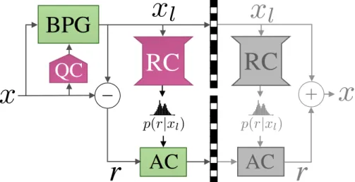
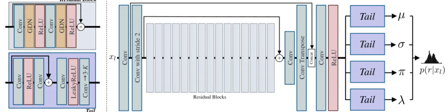
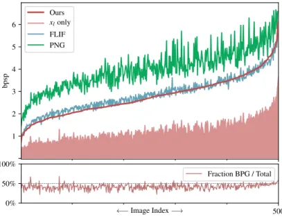
The second lossless algorithm we show is built on top of the powerful lossy image compression algorithm BPG, which outperforms the previously men- tioned approach. In the presented approach, the original image is first decom- posed into the lossy reconstruction obtained after compressing it with BPG and the corresponding residual. We then model the distribution of the residual with a CNN-based probabilistic model that is conditioned on the BPG reconstruction, and combine it with entropy coding to losslessly encode the residual. Finally, the image is stored using the concatenation of the bitstreams produced by BPG and the learned residual coder.

We start the second part of the thesis by addressing one of the challenges of lossy neural image compression: controlling the bitrate of the latent representing the image. We propose a new technique to navigate the rate-distortion trade-off for an compressive auto-encoder. The main idea is to directly model the bitrate of the latent representation by using a “context model”, a 3D-CNN which learns a conditional probability model of the latent distribution of the auto-encoder.

During training, the auto-encoder makes use of the context model to estimate

the bitrate of its representation, and the context model is concurrently updated

to learn the dependencies between the symbols in the latent representation, to

better estimate the probability of the latent representation, and thus the bitrate.

For the final approach, we extensively study how to combine Generative

Adversarial Networks and neural lossy compression to obtain a state-of-the-art

generative lossy compression system. In particular, we investigate normalization

layers, generator and discriminator architectures, training strategies, as well as

perceptual losses. In contrast to previous work, i) we obtain visually pleasing

reconstructions that are perceptually similar to the input, ii) we operate in a

broad range of bitrates, and iii) our approach can be applied to high-resolution

images. We bridge the gap between rate-distortion-perception theory and

practice by evaluating our approach both quantitatively with various perceptual

metrics, and with a user study. The study shows that our method is preferred to

previous approaches even if they use more than 2 × the bitrate.

Z U S A M M E N FA S S U N G

Bildkomprimierung mit neuronalen Netzen wird stetig populärer. In dieser Dissertation präsentieren wir vier Algorithmen für die neuronale Bildkompri- mierung, zwei für verlustfreie Komprimierung und zwei für verlustbehaftete Komprimierung.

Wir beginnen mit dem ersten praxistauglichen gelernten verlustfreien Kom- primierungsalgorithmus, der die populären Algorithmen PNG, WebP, und JPEG2000 übertrifft. Der Algorithmus setzt auf ein komplett parallelisierbares hierarchisches Wahrscheinlichkeitsmodell, das wir für adaptives Arithmetic Co- ding verwenden. Das Model ist ein “Convolutional Neural Network” (CNN, zu dt. etwa “neuronales Faltungsnetzwerk”) und wird end-to-end für die Kompri- mierung gelernt. Wir zeigen, wie dieser Ansatz mit autoregressiven generativen Modellen in Bezug steht, wie zum Beispiel PixelCNN, und wie unser Ansatz Grössenordnungen schneller ist, weil er i) die Wahrscheinlichkeitsverteilung von Bildern zusammen mit den gelernten Repräsentationen lernt, anstatt nur die Bildverteilung im RGB-Raum zu lernen, und ii) nur drei Forwardpasses durch das CNN benötigt, um die Verteilung von jedem Pixel anzugeben, anstatt einen Forwarpass pro Pixel. Dadurch erreichen wir ein bis zu zwei Grössenordnungen schnelleres Sampling als das schnellste PixelCNN (Multiscale-PixelCNN).

Der zweite verlustfreie Algorithmus, den wir zeigen, übertrifft den ersten Algorithmus, indem er auf dem leistungsfähigen verlustbehafteten Bildkom- primierungsalgorithmus BPG aufbaut. Der gezeigte Algorithmus teilt das Ur- sprungsbild in zwei Teile auf: erstens das Ergebnis von BPG, und zweitens das Residuum zwischen diesem Ergebnis und dem Ursprungsbild. Zusammen ergeben die zwei Teile das Ursprungsbild. Wir modellieren dann die Wahrschein- lichkeitsverteilung vom Residuum gegeben dem BPG-Ergebnis mit einem CNN, und kombinieren es wieder mit Arithmetic Coding, um das Residuum verlustfrei zu speichern. Indem wir auch das BPG-Ergebnis speichern, speichern wir das Ursprungsbild so verlustfrei.

Der zweite Teil dieser Dissertation beginnt mit einer Arbeit, die eine der

Herausforderungen im verlustfreien Komprimieren behandelt, nämlich das

Kontrollieren der Bitrate der Repräsentation des Bildes. Wir führen eine neue

Methode ein, die es erlaubt, den Trade-off zwischen Bitrate und Veränderung

des Ausgabebildes (engl. rate-distortion trade-off) mit einem Auto-encoder

zu navigieren. Die Hauptidee ist es, direkt die Bitrate der Repräsentation mit

einem “Context-Modell”, zu modellieren, wofür wir ein 3D-CNN verwenden.

die Abhängigkeiten zwischen den Symbolen der Repräsentation, um deren Wahrscheinlichkeitsverteilung, und somit die Bitrate, besser abzuschätzen. Mit unseren Experimenten zeigen wir, dass unser Ansatz den State of the Art gemessen in MS-SSIM erreicht.

Für den letzten Ansatz untersuchen wir im Detail, wie Generative Adversarial Networks (GANs) mit neuronaler verlustbehafteter Komprimierung kombiniert werden können, um ein State of the Art generatives Komprimierungssystem zu erhalten. Wir untersuchen Normalisierungsarten, Generator- und Discriminator- Architekturen, Trainingsstrategien, sowie Lossfunktionen, die die menschliche Wahrnehmung annähern. Im Gegensatz zu bisherigen Ansätzen i) erhalten wir visuell ansprechende Ausgangsbilder, die sehr nahe am Eingangsbild sind, ii) funktionieren wir in einem breiten Bereich von Bitrates, und iii) funktioniert unser Ansatz für hochaufgelöste Bilder. Wir schliessen die Lücke zwischen

“Rate-distortion-perception” Theorie und Anwendung, indem wir unseren An-

satz sowohl quantitativ mit verschiedenen Metriken als auch mit einer Anwen-

derstudie evaluieren. Die Anwenderstudie zeigt, dass unser Ansatz vorherigen

Ansätzen vorgezogen wird, selbst wenn diese mehr als zweimal so viel Bits

benötigen.

P U B L I C AT I O N S

The following publications are included as a whole or in parts in this thesis:

• Fabian Mentzer et al. “Conditional Probability Models for Deep Im- age Compression.” In: Proceedings of the IEEE/CVF Conference on Computer Vision and Pattern Recognition (CVPR). 2018.

• Fabian Mentzer et al. “Practical Full Resolution Learned Lossless Im- age Compression.” In: Proceedings of the IEEE/CVF Conference on Computer Vision and Pattern Recognition (CVPR). 2019.

• Fabian Mentzer et al. “Learning Better Lossless Compression Using Lossy Compression.” In: Proceedings of the IEEE/CVF Conference on Computer Vision and Pattern Recognition (CVPR). 2020.

• Fabian Mentzer et al. “High-Fidelity Generative Image Compression.” In:

Advances in Neural Information Processing Systems (NeurIPS). 2020.

Furthermore, the following publications were part of my PhD research, but are not covered in this thesis:

• Robert Torfason et al. “Towards Image Understanding from Deep Com- pression Without Decoding.” In: International Conference on Learning Representations (ICLR). 2018.

• Eirikur Agustsson et al. “Soft-to-Hard Vector Quantization for End-to- End Learning Compressible Representations.” In: Advances in Neural Information Processing Systems (NIPS). 2017.

• Eirikur Agustsson et al. “Generative Adversarial Networks for Extreme Learned Image Compression.” In: The IEEE International Conference on Computer Vision (ICCV). 2019.

• Ren Yang et al. “Learning for Video Compression With Hierarchical Quality and Recurrent Enhancement.” In: Proceedings of the IEEE/CVF Conference on Computer Vision and Pattern Recognition (CVPR). 2020.

• Ren Yang et al. “Learning for Video Compression with Recurrent Auto-

Encoder and Recurrent Probability Model.” Under Review. 2020.

AC K N OW L E D G M E N T S

I would like to thank Prof. Luc Van Gool for giving me the opportunity to pursue a PhD in his lab. Thanks to him, I was able to freely choose research directions that interested me, while being financially supported. I would like to thank Radu Timofte for believing in me and supporting my work. The environment of the lab helped me to stay focused and motivated, and I spent many great hours there.

This thesis would not have been possible without my two close collaborators, Eirikur Agustsson and Michael Tschannen. I met Michael when I was doing my master, where he supervised my second semester thesis. Supervised by him and Eirikur, I wrote my master thesis, and since then our collaboration has been steadily going throughout the PhD. Without their insightful comments and relentless persistence, this work would not have been possible.

I would like to thank Sergi Caelles, for making the days at the lab brighter with discussions, and for helping me with tough decisions. I would like to thank Kevis Maninis for helping me settle into PhD life with his advice early in the studies. The final work presented in this thesis was done during an internship at Google, and I would like to thank George Toderici for the many hours he spent supporting the paper. Without him, we would not have the thorough user study that we have now, and the paper would be overall less solid. I would like to thank Luisa Blom for supporting me mentally through many tough deadlines. I would like to thank my family for the thorough support throughout my studies.

Thanks to them, I was able to focus on my studies.

C O N T E N T S

1 I N T RO D U C T I O N 1

1.1 Lossless Image Compression . . . . 2

1.2 Lossy Image Compression . . . . 3

2 B AC K G RO U N D 5 2.1 Rate Loss and Information Theory . . . . 5

2.2 Adaptive Arithmetic Coding . . . . 7

Part I L O S S L E S S A L G O R I T H M S 9 3 R E L AT E D W O R K O N L O S S L E S S C O M P R E S S I O N 11 3.1 Learned Lossless Compression . . . . 11

3.2 Likelihood-Based Generative Models . . . . 11

3.3 Engineered Codecs . . . . 12

3.4 Context Models in Lossy Compression . . . . 12

3.5 Continuous Likelihood Models for Compression . . . . 12

4 P R AC T I C A L F U L L R E S O L U T I O N L E A R N E D L O S S L E S S I M - AG E C O M P R E S S I O N 15 4.1 Overview . . . . 15

4.2 Method . . . . 17

4.3 Experiments . . . . 23

4.4 Results . . . . 25

4.5 Conclusion . . . . 29

4.A Encoding and Decoding Details . . . . 30

4.B Comparison on ImageNet64 . . . . 33

4.C Note on Comparing Times for 32 × 32 Images . . . . 33

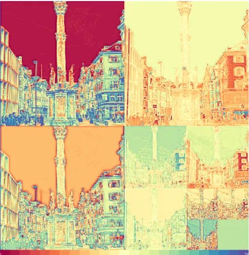
4.D Visualizing Representations . . . . 35

4.E Architectures of Baselines . . . . 36

5 L E A R N I N G B E T T E R L O S S L E S S C O M P R E S S I O N U S I N G L O S S Y C O M P R E S S I O N 39 5.1 Overview . . . . 39

5.2 Related Work . . . . 41

5.3 Proposed Method . . . . 42

5.4 Experiments . . . . 48

5.5 Results and Discussion . . . . 50

5.6 Conclusion . . . . 53

5.A Q-Classifier Architecture . . . . 54

5.B BPG Performance . . . . 54

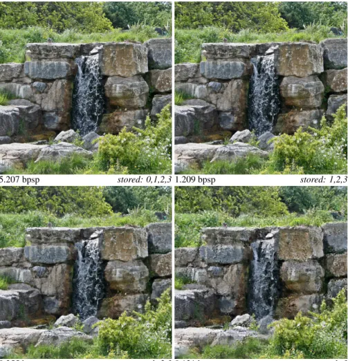
5.C Examples from the testing sets . . . . 55

Part II L O S S Y A L G O R I T H M S 57 6 C O N D I T I O N A L P RO B A B I L I T Y M O D E L S F O R D E E P I M AG E C O M - P R E S S I O N 59 6.1 Overview . . . . 59

6.2 Related work . . . . 61

6.3 Compressive Auto-encoder . . . . 62

6.4 Proposed method . . . . 62

6.5 Experiments . . . . 68

6.6 Discussion . . . . 73

6.7 Conclusions . . . . 75

6.A Visual examples . . . . 76

6.B 3D probability classifier . . . . 81

7 H I G H - FI D E L I T Y G E N E R AT I V E I M AG E C O M P R E S S I O N 83 7.1 Introduction . . . . 83

7.2 Related work . . . . 85

7.3 Method . . . . 87

7.4 Experiments . . . . 91

7.5 Results . . . . 94

7.6 Conclusion . . . . 99

7.A Comparing MSE models based on Minnen et al. [69] . . . . . 100

7.B Using LPIPS without a GAN loss . . . . 101

7.C Qualitative Comparison to Previous Generative Approaches . . 102

7.D ChannelNorm . . . . 104

7.E Further Results on User Study . . . . 105

7.F Further Quantitative Results . . . . 108

7.G Implementation Details . . . . 110

7.H Further Visual Results . . . . 112

8 D I S C U S S I O N 113 8.1 Summary of Contributions . . . . 113

8.2 Limitations and Future Work . . . . 114

B I B L I O G R A P H Y 117

1

I N T RO D U C T I O N

In the time since the wide-spread adoption of smartphones with high-quality cameras, the number of images taken every year is increasing, having reached an estimated 1 trillion images in 2015 [79]. Typical smartphone sensors today contain roughly 12 million pixels (e.g., the iPhone 12’s cameras [39]). In a standard setup, each pixel captures red, green, and blue intensities (RGB), and supports 256 possible values for each color, which can be represented with 8 bits per color, or 24 bits per pixel. Thus, an uncompressed 12 MP image would require roughly 36 megabytes to store. Since this is impractically large, image compression algorithms are employed. Instead of storing the raw value of each pixel of the camera sensor with 24 bits, the image is converted to a more

“compressible” representation first. We can broadly distinguish two categories:

In lossless image compression, the input image is reconstructed pixel-perfectly.

These algorithms exploit redundancy and other structures of images to reduce the number of bits needed to store the image (“bitrate” for short). In lossy image compression, the reconstructed image is allowed to be different from the input.

Here, in addition to exploiting redundancy, approaches focus on trading off bitrate with how “good” the reconstruction is. This effectively means that the compression algorithm is allowed to throw away hard-to-compress structure or texture. Intuitively, the more bits, the closer the reconstruction can be to the input. This latter class of algorithms is what is in widespread use, a prominent example being JPEG [106]. However, lossless compression algorithms are also frequently used, e.g., in professional photography or medical imaging.

Recently, deep neural networks have been employed for image compression.

The idea is to formulate the image compression problem via a suitable loss function, and to parametrize the “compression algorithm” with a neural network.

By training this neural network on a sufficiently large corpus of images we can obtain compression algorithms that outperform their non-learned predecessors.

The key questions that naturally arise are i) which loss function to use, and ii) which neural network to use. While the first question has an obvious answer for lossless algorithms (the bitrate is all we can minimize, as pixel-perfect reconstruction is a hard requirement), it is non-obvious for lossy algorithms.

Intuitively, we are looking for lossy image compression algorithms that only

throw away parts of the image that a human observer does not notice, and that do

not introduce any obvious compression artifacts, i.e., we are looking for a loss

function that captures how humans perceive reconstructions. As an example,

x

E y D

x

Lossless Coding using p(y)

. . . 10111010 . . .

Figure 1.1: High-level schematic of the auto-encoder structure commonly used in neural lossy image compression. The image x is fed through an encoder network E to obtain the representation y, which is written to disk losslessly using the learned probability distribution p(y). From y, we can obtain the reconstruction x

using the decoder D.

humans generally do not care if the leaves of a tree face slightly different directions in the reconstruction as long as the tree type, color, lighting, and so on are still the same. If we had such a human-perception-based loss function, we could backpropagate through it to learn perfect compression algorithms.

Alas, we do not have such a function, and recent efforts in neural lossy image compression have focused on approximating it.

Regarding the second question, which neural network to use, the general structure on a high level is similar for many lossy compression works, and shown in Fig. 1.1: A representation y of the image x is learned by training a convolutional neural network (CNN)-based auto-encoder (E, D), and the representation y is compressed by training a second neural network to approxi- mate its probability distribution p(y). For lossless compression works, fewer approaches exists, and they differ more significantly in structure, as we shall see later.

In this thesis, we present neural network-based image compression ap- proaches for both the lossless and the lossy regime.

1.1 L O S S L E S S I M AG E C O M P R E S S I O N

Lossless image compression focuses on leveraging redundancies in natural images to save bits. For example, PNG [81] is based on simple autoregressive filters that update pixels based on surrounding pixels, allowing for efficient compression of, e.g., uniform image regions. There has been comparatively little work on using neural networks for lossless image compression specifically.

However, the generative modelling literature is inherently related to the problem.

There, the goal is to learn representations of images and to sample new images,

1.2

both of which is achieved by learning probability models of real images. An example in this category is PixelCNN [76]. Such a model can in theory be used for lossless compression, by pairing it with a entropy coding algorithm. After all (as we will also see in this thesis), all we need for lossless compression is a probability distribution of the data you are trying to compress, and an entropy coding algorithm that transforms data to a bitstream, using the distribution.

While such approaches can be used for lossless compression, state-of-the- art generative models rely on autoregressive factorizations and are too slow for the task. We discuss this in Part I of this thesis, where we present two approaches to neural network-based lossless image compression. The first approach (Ch. 4) learns a hierarchical auto-encoder that decomposes the input image into a sequence of ever smaller representations. We then use smaller representations to predict the probability distribution of bigger representations recursively. By training the network to minimize bitrate, we learn good models of the probability distributions, and are able to efficiently store images. In the second approach (Ch. 5), we leverage the lossy image compression algorithm BPG for lossless compression, by learning the distribution of residuals with a neural network.

1.2 L O S S Y I M AG E C O M P R E S S I O N

A well-known and widely-used lossy image compression algorithm is JPEG [106], introduced in 1980. Since then, numerous alternatives have been proposed, including JPEG2000 [95], WebP [111], and, recently, BPG [9], which is based on the state-of-the-art video codec HEVC [93]. Around 2015, deep neural net- works (DNNs) trained for image compression led to promising results [99, 101, 97, 7, 1, 58], achieving better performance than many traditional techniques for image compression. These approaches are directly minimizing the desired trade-off. Initial works focused on minimizing the “rate-distortion” trade-off r + λd, where d is a pairwise (between pairs of images) distortion metric (e.g., mean-squared error (MSE), or the Multi-Scale Structural Similarity Metric (MS-SSIM)) which measures how close is the reconstruction to the input. Later work also takes perceptual quality d

into account [3, 11], which measures how “realistic” the output looks, regardless of how close it is to the input, by measuring a divergence d

between the distribution p

of real images and the distribution of reconstructions p

, giving rise to the triple “rate-distortion- perception” trade-off r + λd + βd

[11]. Such a loss nicely approximates human preferences without requiring an exact mathematical expression for it.

In Part II we present two approaches for neural network-based lossy image

compression. The first approach (Ch. 6) studies the rate-distortion setting, and

focuses on minimizing the rate R with a sophisticated entropy model. The goal

is to model the distribution of the image representation, to be able to efficiently

store that representation with entropy coding. The second approach (Ch. 7)

studies the rate-distortion-perception setting, and uses a GAN loss to improve

the perceptual quality of reconstructions.

2

BAC K G RO U N D

2.1 R AT E L O S S A N D I N F O R M AT I O N T H E O RY

One common theme of the four works we present in the following is that all algorithms eventually compress a stream of symbols s = (s

, . . . , s

) losslessly. In Ch. 4, we compress the RGB image and a set of auxiliary variables, in Ch. 5 we compress the RGB residual, and in Ch. 6, 7, we compress the latent variables. To do this, we always approximate the real (unkown) distribution q(s) of the symbols with a model p(s), and we use an entropy coding algorithm (adaptive arithmetic coding to be precise, see below) to encode the symbols to the bitstream.

The underlying intuition from Information Theory is that the more we know about the distribution of the symbols, the more efficient we can compress them, by assigning shorter bit-sequences to more likely symbols.

Doing this will yield short average bitstreams.

To minimize the number of bits we use, we always add a rate loss L

to whatever objective we have. By minimizing L

, we minimize the bits needed to store s , where

L

= E

[ − log p(s)] (2.1) is a cross-entropy between the real distribution q(s) and the model p(s).

In this section, we want to briefly show how this loss can be derived using simple information theory tools. We want to highlight that we consider com- pressing the entire s at once, instead of compressing its parts s

. In contrast to what we usually see in Information Theory theorems, we do not model the s

as identically distributed. Instead, in our setup, the representations s

, s

of different images a, b are independent and identically distributed.

We can model the symbol stream as a random variable S = (S

, . . . , S

) , where each S

is also a random variable, that takes value in the finite set S.

We denote the (unknown) joint distribution with q(S), and the (unknown)

1 We note that in the literature, e.g., in Cover & Thomas [21], the real distribution is more

commonly denoted with p, reserving q for the model. We flip this notation as we are mainly

interested in the model throughout the following chapters.

distribution of individual symbols S

with q

(S

) . The symbols S have the following joint entropy:

H(q(S)) =H(q

(S

)) + H(q

(S

) | q

(S

)) + · · · +

H(q

(S

) | q

(S

), . . . , q

(S

)) (2.2) Note that we cannot simplify this further without making assumptions about q(S ) , and that q(S) specifies the probability of many possible symbol streams, as it specifies the probability for each possible realization s, and there are |S|

such realizations.

We are interested in encoding realizations of S losslessly into a bitstream, such that they can be recovered exactly.

Let L

be the expected minimum code length, as in [21, Theorem 5.4.1, p113]. From that Theorem, we know that

H(q(S )) ≤ L

< H(q(S)) + 1. (2.3) Note that here, we consider the whole stream S, and L

is the expected mini- mum code length to encode one realization s . While this code length might be shorter than H(S ) for one particular realization, the lemma says that we cannot go below the entropy in expectation.

However, as mentioned, in general we do not know the real underlying distribution q(S) . Instead, we introduce a model p of q . Following [21, Theorem 5.4.3, p115], we know that using p(S) to encode a sequence S that is actually distributed according to q(S) incurs an overhead of

L ¯ = D

(q(S), p(S )) bits, (2.4) and the overall expected code length r becomes

r = L

+ ¯ L < 1 + H(q(S )) + D

(q(S), p(S))

= 1 + E

[ − log p(S)]

| {z }

cross-entropy

, (2.5)

which shows that we can in fact minimize L

in Eq. 2.1 to minimize the expected rate.

2 For a typical compressive auto-encoder (e.g., Ballé et al., 2018, [8]), and a moderately large

image of 768×512 pixels, s will have N = 768/8 · 512/8 · 192 = 1 179 648 entries already.

2.2

In Ch. 4, 5, and 7, we introduce a conditional independence assumption into the model p. In particular, we decompose S into two parts, a side-information Z, and the latents S

, where

p(S) = p(S

, Z) = p(Z)p(S

| Z) = p(Z) · Y

i

p

(S

| Z).

We first encode Z using p(Z), and then encode the elements S

of S

condition- ally independent with their models p

(S

| Z). We note that Eq. 2.5 still holds, but can be extended to

r < 1 + E

[ − log p(Z)] + E

[ − log p(S

| Z)], (2.6) where q now represents the unknown joint distribution q(S

, Z).

2.2 A DA P T I V E A R I T H M E T I C C O D I N G

To actually encode a realization s into a bitstream, a so called “entropy coding algorithm” can be used. The idea of these algorithms is to use a probability distribution model p to efficiently encode symbols, since p allows the coder to assign shorter bit-sequences to more likely symbols. Depending on the implementation, these algorithms may incur a non-negligible bit-overhead. For example, Huffman coding [37] only achieves optimal rates for probabilities p

(S

) that are powers of two. To allow more flexible models, we use adaptive arithmetic coding in all presented works.

Adaptive Arithmetic Coding [113] is a strategy that almost achieves the theoretical rate bound from above (for long enough symbol streams). It encodes the entire stream into a single number a

∈ [0, 1) , by subdividing [0, 1) in each step (a step means encoding one symbol) as follows: Let a, b be the bounds of the current step (initialized to a = 0 and b = 1 for the initial interval [0, 1)). We divide the interval [a, b) into |S| sections where the length of the j -th section is p

(S

)/(b − a) (the algorithms is called adaptive because it allows different p

for different symbols). Then we pick the interval corresponding to the current

symbol, i.e., we update a, b to be the boundaries of this interval. We proceed

recursively until no symbols are left. Finally, we transmit a

, which is a rounded

to the smallest number of bits s.t. a

≥ a. Receiving a

together with the

knowledge of the number of encoded symbols and p uniquely specifies the

stream and allows the receiver to recover the symbols perfectly.

PART I

L O S S L E S S A L G O R I T H M S

3

R E L AT E D W O R K O N L O S S L E S S C O M P R E S S I O N

3.1 L E A R N E D L O S S L E S S C O M P R E S S I O N

The work we present in Chapter 4 was the first work to present a neural network based algorithm for lossless image compression that worked at high resolu- tions in practical runtimes. Other work focused on smaller data sets such as MNIST [54], CIFAR-10 [51], and ImageNet32/64 [18], where they achieve state-of-the-art results. In particular, Townsend et al. [103] and Kingma et al. [48] leverage the “bits-back scheme” [34] for lossless compression of an image stream, where the overall bitrate of the stream is reduced by leveraging previously transmitted information. Motivated by progress in generative model- ing using (continuous) flow-based models (e.g., [83, 47]), Hoogeboom et al. [35]

propose Integer Discrete Flows (IDFs), defining an invertible transformation for discrete data.

3.2 L I K E L I H O O D - B A S E D G E N E R AT I V E M O D E L S

Essentially all likelihood-based discrete generative models can be used with an arithmetic coder for lossless compression. A prominent group of models that obtain state-of-the-art performance are variants of the auto-regressive PixelRN- N/PixelCNN [76, 75]. PixelRNN and PixelCNN organize the pixels of the image distribution as a sequence and predict the distribution of each pixel conditionally on (all) previous pixels using an RNN and a CNN with masked convolutions, respectively. These models hence require a number of network evaluations equal to the number of predicted sub-pixels

(3 · W · H). PixelCNN++ [88]

improves on this in various ways, including modeling the joint distribution of each pixel, thereby eliminating conditioning on previous channels and reduc- ing to W · H forward passes. MS-PixelCNN [82] parallelizes PixelCNN by reducing dependencies between blocks of pixels and processing them in parallel with shallow PixelCNNs, requiring O(log W H ) forward passes. Kolesnikov et al. [50] equip PixelCNN with auxiliary variables (grayscale version of the image or RGB pyramid) to encourage modeling of high-level features, thereby improving the overall modeling performance. Chen et al. [17], and Parmar et

3 A RGB “pixel” has 3 “sub-pixels”, one in each channel.

al. [78] propose autoregressive models similar to PixelCNN/PixelRNN, but they additionally rely on attention mechanisms to increase the receptive field.

3.3 E N G I N E E R E D C O D E C S

The well-known PNG [81] operates in two stages: first the image is reversibly transformed to a more compressible representation with a simple autoregressive filter that updates pixels based on surrounding pixels, then it is compressed with the deflate algorithm [23]. WebP [111] uses more involved transformations, including the use of entire image fragments to encode new pixels and a custom entropy coding scheme. JPEG2000 [95] includes a lossless mode where tiles are reversibly transformed before the coding step, instead of irreversibly removing frequencies. The current state-of-the-art (non-learned) algorithm is FLIF [92].

It relies on powerful preprocessing and a sophisticated entropy coding method based on CABAC [84] called MANIAC, which grows a dynamic decision tree per channel as an adaptive context model during encoding.

3.4 C O N T E X T M O D E L S I N L O S S Y C O M P R E S S I O N

In lossy compression, context models have been studied as a way to efficiently losslessly encode the obtained image representations. Classical approaches are discussed in [62, 67, 68, 114, 112]. Recent learned approaches include [58, 63, 69], where shallow autoregressive models over latents are learned. Ballé et al. [8] present a model somewhat similar to the work presented next: Their auto-encoder is similar to our fist scale, and the hyper encoder/decoder is similar to our second scale. However, since they train for lossy image compression, their auto-encoder predicts RGB pixels directly. Also, they predict uncertainties σ for the latent instead of a mixture of logistics. Finally, instead of learning a probability distribution for their “hyper-latent” ( z

in our formulation), they assume the entries to be i.i.d. and fit a univariate non-parametric density model, whereas in our model, many more stages can be trained and applied recursively.

3.5 C O N T I N U O U S L I K E L I H O O D M O D E L S F O R C O M P R E S S I O N

The objective of continuous likelihood models, such as VAEs [45] and RealNVP

[24], where p(x

) is a continuous distribution, is closely related to its discrete

counterpart. In particular, by setting x

= x + u where x is the discrete image

and u is uniform quantization noise, the continuous likelihood of p(x

) is a

lower bound on the likelihood of the discrete p(x) = ˆ E

[p(x

)] [96]. However,

there are two challenges for deploying such models for compression. First,

3.5

the discrete likelihood p(x) ˆ needs to be available (which involves a non-trivial

integration step). Additionally, the memory complexity of (adaptive) arithmetic

coding depends on the size of the domain of the variables of the factorization

of p ˆ (see Sec. 2.2 on (adaptive) arithmetic coding). Since the domain grows

exponentially in the number of pixels in x, unless p ˆ is factorizable, it is not

feasible to use it with adaptive arithmetic coding.

4

P R AC T I C A L F U L L R E S O L U T I O N L E A R N E D L O S S L E S S I M AG E C O M P R E S S I O N

We propose the first practical learned lossless image compression system, named L3C, and show that it outperforms the popular engineered codecs, PNG, WebP and JPEG2000. At the core of our method is a fully parallelizable hierarchical probabilistic model for adaptive entropy coding which is optimized end-to-end for the compression task. In contrast to recent autoregressive discrete proba- bilistic models such as PixelCNN, our method i) models the image distribution jointly with learned auxiliary representations instead of exclusively modeling the image distribution in RGB space, and ii) only requires three forward-passes to predict all pixel probabilities instead of one for each pixel. As a result, L3C obtains over two orders of magnitude speedups when sampling compared to the fastest PixelCNN variant (Multiscale-PixelCNN). Furthermore, we find that learning the auxiliary representation is crucial and outperforms predefined auxiliary representations such as an RGB pyramid significantly.

4.1 OV E RV I E W

Our system (see Fig. 4.1 for an overview) is based on a hierarchy of fully parallel learned feature extractors and predictors which are trained jointly for the compression task. Our code is available online.

The role of the feature extractors is to build an auxiliary hierarchical feature representation which helps the predictors to model both the image and the auxiliary features themselves. Our experiments show that learning the feature representations is crucial, and heuristic (predefined) choices such as a multiscale RGB pyramid lead to suboptimal performance.

In more detail, to encode an image x, we feed it through the S feature extractors E

and predictors D

. Then, we obtain the predictions of the probability distributions p, for both x and the auxiliary features z

, in parallel in a single forward pass. These predictions are then used with an adaptive arithmetic encoder to obtain a compressed bitstream of both x and the auxiliary features (Sec. 2.2 provides an introduction to arithmetic coding). However, the arithmetic decoder now needs p to be able to decode the bitstream. Starting from the lowest scale of auxiliary features z

, for which we assume a uniform prior, D

obtains a prediction of the distribution of the auxiliary features of

4 github.com/fab-jul/L3C-PyTorch

<latexit sha1_base64="06rEWvWPE+mR3cLra/xJ60akb/c=">AAAKdHicvVZbb9MwGM3GZV0YsAFv8GCoJnWsq5JymzQqTdoDPA6JXaQkmhzHac0cJ3IcttbKz+GVR/4Lj/wJnrGTDbreNECNq0qfv/PZx+fE0mc/oSQVlvV9YfHGzVu3l2rL5p2Vu/fur649OEzjjCN8gGIa82MfppgShg8EERQfJxzDyKf4yD/d0/jRZ8xTErOPop9gL4JdRkKCoFCpk7WlL6br4y5hUpDTQUKQyDjOHb0d+BQT1uFxxgLPdJNuGEHRS7GIIOKxdFHm4/Nc2vkUrD8DG+TSalmvJsFxGKqJxtvTYV/jL6fjSOOvp+OBxrcVHnB45mRUcAhEj7BmSCjt7KkTFs55oGE11W8DbG2Bzc3GVil6OGU1y2T/T2qkCPURxTt/S6Un5c6DGVS6aqjo36gmqhpj/x9VF65XZ+MI4fzNvI7CeVjqV+6pX7mpszXOw1VUuauocldna5yHq0HlrgaVuzpb43VdxSy40o5N82S1rhpmMcB4YF8E9d1669Hgx7uv+ydrC9/cIEZZhJlAFKapY1uJ8CTkgigS1fqyFCcQncIudlTIYIRTTxYPihysq0wAwpirPxOgyA6vkDBK037kq8qivY5iOjkRO78kGIf8aFLayUS47UnCkkxghsqjhRkFIgb6PQMCwjEStK8C1eGJUgdQD3KIhHr1XCHQjirdDJ+hOIogC567iHBlRuDYnnQ17Fw+pToNvUlLTzc8aYKh4bI4wE7agwnulOvLG3HWIwI39WVpEsYwB4q501aeg2KvDSDrdr6TqxMUHlAs5O9LlEufqlM+ta1cfWl79LuOB4ftlv2i1f5g13fbRjlqxmPjmdEwbOONsWu8N/aNAwPVVmrt2k7t7fJP84lZN9fL0sWFizUPjSvDbP0C1iAzRg==</latexit>

<latexit sha1_base64="u3Q1uGUfKwtLn7PsOvnF1uOcuVk=">AAAHVnictVXdbtMwFM7Guo7CYAVuJm4MFVLHuirpkEAalSZxw+WQ2I+URJPjnLRmjh05Dl0X5TkQPADPBC+DsJtN69auYmM7UaTj8x2fz+eLdRIkjKbKtn/Pzd9bqCxWl+7XHjxcfvR4pf5kLxWZJLBLBBPyIMApMMphV1HF4CCRgOOAwX5w9MHg+19BplTwz2qYgB/jHqcRJVjp0GF94WfNC6BHea7o0UlCicokFK4ph74IyrtSZDz0a17Si2Ks+imoGBMpco9kARwXuVNcgQ1nYCdFbrenoiKK9MLAnavhwOBvNB5KPHAzpiRGqk95K6KMdQOWwQvH9lHTbulnDW1soPX15kZ54vGQ3SqDw/PQpSQyJAy2rkdkFmXdkxlEJmss6SZEUzua4L5ORz0JwM+ZTuW+OwVn892+kDfo77/0lBBOsAV3J+dMuttX8/rd/auYwMML86hWO1xp2G17ZGjScU6dxvbq6ndtP3YO63PfvFCQLAauCMNp6jp2ovwcS0U1iR4eWQoJJke4B652OY4h9fPRRC3QKx0JUSSkfrlCo+j4jhzHaTqMA505GlCXMROcih2fEUxCQTwt7GYqeufnlCeZAk7Ko0UZQ0ogM9BRSCUQxYba0TOS6u4Q6WOJidJj/wKBUVT3zWFARBxjHr72CJVajNB1/NwzsHv2L+k2TZG2Wa75eQ2NmcdFCG7axwl0y/3ldRj0qYKWuSktyjlIpJm7Ha05GtVaQ3nDKbaKQn9K5/KHm3T2Om1ns9355DS2n1mlLVnPrZdW03Kst9a29dHasXYtUlmubFbeV7qLvxb/VCvVapk6P3e656l1waorfwE0mTsw</latexit> <latexit sha1_base64="06rEWvWPE+mR3cLra/xJ60akb/c=">AAAKdHicvVZbb9MwGM3GZV0YsAFv8GCoJnWsq5JymzQqTdoDPA6JXaQkmhzHac0cJ3IcttbKz+GVR/4Lj/wJnrGTDbreNECNq0qfv/PZx+fE0mc/oSQVlvV9YfHGzVu3l2rL5p2Vu/fur649OEzjjCN8gGIa82MfppgShg8EERQfJxzDyKf4yD/d0/jRZ8xTErOPop9gL4JdRkKCoFCpk7WlL6br4y5hUpDTQUKQyDjOHb0d+BQT1uFxxgLPdJNuGEHRS7GIIOKxdFHm4/Nc2vkUrD8DG+TSalmvJsFxGKqJxtvTYV/jL6fjSOOvp+OBxrcVHnB45mRUcAhEj7BmSCjt7KkTFs55oGE11W8DbG2Bzc3GVil6OGU1y2T/T2qkCPURxTt/S6Un5c6DGVS6aqjo36gmqhpj/x9VF65XZ+MI4fzNvI7CeVjqV+6pX7mpszXOw1VUuauocldna5yHq0HlrgaVuzpb43VdxSy40o5N82S1rhpmMcB4YF8E9d1669Hgx7uv+ydrC9/cIEZZhJlAFKapY1uJ8CTkgigS1fqyFCcQncIudlTIYIRTTxYPihysq0wAwpirPxOgyA6vkDBK037kq8qivY5iOjkRO78kGIf8aFLayUS47UnCkkxghsqjhRkFIgb6PQMCwjEStK8C1eGJUgdQD3KIhHr1XCHQjirdDJ+hOIogC567iHBlRuDYnnQ17Fw+pToNvUlLTzc8aYKh4bI4wE7agwnulOvLG3HWIwI39WVpEsYwB4q501aeg2KvDSDrdr6TqxMUHlAs5O9LlEufqlM+ta1cfWl79LuOB4ftlv2i1f5g13fbRjlqxmPjmdEwbOONsWu8N/aNAwPVVmrt2k7t7fJP84lZN9fL0sWFizUPjSvDbP0C1iAzRg==</latexit>

D ⁽¹⁾ E ⁽¹⁾

D ⁽¹⁾

E ⁽¹⁾ D ⁽²⁾

D ⁽³⁾ E ⁽³⁾

x z

z

z

Q

Q

Q

E ⁽²⁾

f⁽³⁾ f⁽²⁾ f⁽¹⁾

p(z⁽²⁾|f⁽³⁾)

p(z⁽¹⁾|f⁽²⁾)

p(x | f

)

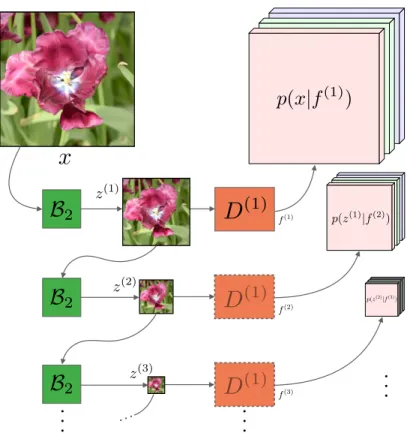
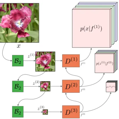
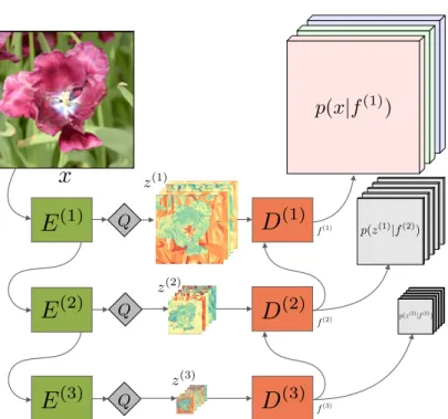
Figure 4.1: Overview of the architecture of L3C. The feature extractors

E

compute quantized (by Q) auxiliary hierarchical feature representation

z

, . . . , z

whose joint distribution with the image x, p(x, z

, . . . , z

),

is modeled using the non-autoregressive predictors D

. The features f

summarize the information up to scale s and are used to predict p for the next

scale.

4.2

the next scale, z

, and can thus decode them from the bitstream. Prediction and decoding is alternated until the arithmetic decoder obtains the image x.

In practice, we only need to use S = 3 feature extractors and predictors for our model, so when decoding we only need to perform three parallel (over pixels) forward passes in combination with the adaptive arithmetic coding.

The parallel nature of our model enables it to be orders of magnitude faster for decoding than autoregressive models, while learning enables us to obtain compression rates competitive with state-of-the-art engineered lossless codecs.

4.2 M E T H O D

The general lossless compression setting is described in Ch. 2. We describe the method specific details here.

4.2.1 Architecture

A high-level overview of the architecture is given in Fig. 4.1, while Fig. 4.2 shows a detailed description for one scale s. Unlike autoregressive models such as PixelCNN and PixelRNN, which factorize the image distribution autoregres- sively over sub-pixels x

as p(x) = Q

t=1

p(x

| x

, . . . , x

) , we jointy model all the sub-pixels and introduce a learned hierarchy of auxiliary feature repre- sentations z

, . . . , z

to simplify the modeling task. We fix the dimensions of z

to be C × H

× W

, where the number of channels C is a hyperparameter (C = 5 in our reported models), and H

= H/2

, W

= W/2

given a H × W - dimensional image.

Specifically, we model the joint distribution of the image x and the feature representations z

as

p(x, z

, . . . , z

) = p(x | z

, . . . , z

)

S

Y

s=1

p(z

| z

, . . . , z

)

where p(z

) is a uniform distribution. The feature representations can be hand designed or learned. Specifically, on one side, we consider an RGB pyramid with z

= B

(x), where B

is the bicubic (spatial) subsampling operator with subsampling factor 2

. On the other side, we consider a learned represen- tation z

= F

(x) using a feature extractor F

. We use the hierarchical model shown in Fig. 4.1 using the composition F

= Q ◦ E

◦ · · · ◦ E

, where the E

are feature extractor blocks and Q is a scalar differentiable

5 Considering that z

is quantized, this choice conveniently upper bounds the information that

can be contained within each z

, however, other choices could be explored.

CTICALFULLRESOLUTIONLEARNEDLOSSLESSIMAGECOMPRESSION

Q

C E^(s)_in

E_in^(s+1)

4Cf

s2f5

s1f1

s1f1 s1f1

E

D

f^(s)

p(z^{(s 1)}|f^(s))

z^(s)

U A⇤ ReLU

C^(s_p ¹⁾

⇡,µ,

f^(s+1)

f^(s)

+ +

+ +

Figure 4.2: Architecture details for a single scale s. For s = 1, E

is the RGB image x normalized to [ − 1, 1]. All vertical black

lines are convolutions, which have C

= 64 filters, except when denoted otherwise beneath. The convolutions are stride 1 with

3 × 3 filters, except when denoted otherwise above (using sSfF = stride s, filter f ). We add the features f

from the predictor

D

to those of the first layer of D

(a skip connection between scales). The gray blocks are residual blocks, shown once

on the right side. C is the number of channels of z

, C

is the final number of channels, see Sec. 4.2.3. Special blocks

are denoted in red: U is pixelshuffling upsampling [90]. A ∗ is the “atrous convolution” layer described in Sec. 4.2.1. We use a

heatmap to visualize z

, see Sec. 4.D.

4.2

quantization function (see Sec. 4.2.2). The D

in Fig. 4.1 are predictor blocks, and we parametrize E

and D

as convolutional neural networks.

Letting z

= x, we parametrize the conditional distributions for all s ∈ { 0, . . . , S } as

p(z

| z

, . . . , z

) = p(z

| f

),

using the predictor features f

= D

(f

, z

).

Note that f

sum- marizes the information of z

, . . . , z

.

The predictor is based on the super-resolution architecture from EDSR [60], motivated by the fact that our prediction task is somewhat related to super- resolution in that both are dense prediction tasks involving spatial upsampling.

We mirror the predictor to obtain the feature extractor, and follow [60] in not using BatchNorm [38]. Inspired by the “atrous spatial pyramid pooling” from Chen et al. [16], we insert a similar layer at the end of D

, which we call

“ A ∗”. We use three atrous convolutions in parallel, with rates 1, 2, and 4, then concatenate the resulting feature maps to a 3C

-dimensional feature map.

4.2.2 Quantization

We use a scalar quantization approach based on the vector quantization approach proposed by Agustsson et al. [1], to quantize the output of E

: Given levels L = { `

, . . . , `

} ⊂ R, we use nearest neighbor assignments to quantize each entry z

∈ z

as

z = Q(z

) := arg min

k z

− `

k , (4.1) but use differentiable “soft quantization”

Q(z ˜

) =

L

X

j=1

`

exp( − σ

k z

− `

k ) P

l=1

exp( − σ

k z

− `

k ) (4.2) to compute gradients for the backward pass, where σ

is a hyperparameter relating to the “softness” of the quantization. For simplicity, we fix L to be L = 25 evenly spaced values in [ − 1, 1].

4.2.3 Mixture Model

For ease of notation, let z

= x again. We model the conditional distribu- tions p(z

| z

, . . . , z

) using a generalization of the discretized logistic

6 The final predictor only sees z

, i.e., we let f

= 0.

mixture model with K components proposed in [88], as it allows for efficient training: The alternative of predicting logits per (sub-)pixel has the downsides of requiring more memory, causing sparse gradients (we only get gradients for the logit corresponding to the ground-truth value), and does not model that neighbouring values in the domain of p should have similar probability.

Let c denote the channel and u, v the spatial location. For all scales, we assume the entries of z

to be independent across u, v , given f

. For RGB (s = 0), we define

p(x | f

) = Y

u,v

p(x

, x

, x

| f

), (4.3) where we use a weak autoregression over RGB channels to define the joint probability distribution via a mixture p

(dropping the indices uv for shorter notation):

p(x

, x

, x

| f

) = p

(x

| f

) · p

(x

| f

, x

) ·

p

(x

| f

, x

, x

). (4.4) We define p

as a mixture of logistic distributions p

(defined in Eq. (4.9) below). To this end, we obtain mixture weights

π

, means µ

, variances σ

, as well as coefficients λ

from f

(see further below), and get

p

(x

| f

) = X

k

π

p

(x

| µ ˜

, σ

) p

(x

| f

, x

) = X

k

π

p

(x

| µ ˜

, σ

) p

(x

| f

, x

, x

) = X

k

π

p

(x

| µ ˜

, σ

), (4.5) where we use the conditional dependency on previous x

to obtain the updated means µ, as in [88, Sec. 2.2], ˜

˜

µ

= µ

µ ˜

= µ

+ λ

x

˜

µ

= µ

+ λ

x

+ λ

x

. (4.6) Note that the autoregression over channels in Eq. (4.4) is only used to update the means µ to µ. ˜

7 Note that in contrast to [88] we do not share mixture weights π

across channels. This allows for

easier marginalization of Eq. (4.4).

4.2

For the other scales ( s > 0 ), the formulation only changes in that we use no autoregression at all, i.e., µ ˜

= µ

for all c, u, v. No conditioning on previous channels is needed, and Eqs. (4.3)-(4.5) simplify to

p(z

| f

) = Y

c,u,v

p

(z

| f

) (4.7) p

(z

| f

) = X

k

π

p

(z

| µ

, σ

). (4.8)

For all scales, the individual logistics p

are given as p

(z | µ, σ) = sigmoid((z + b/2 − µ)/σ) −

sigmoid((z − b/2 − µ)/σ)

. (4.9)

Here, b is the bin width of the quantization grid (b = 1 for s = 0 and b = 1/12 otherwise). The edge-cases z = 0 and z = 255 occurring for s = 0 are handled as described in [88, Sec. 2.1].

For all scales, we obtain the parameters of p(z

| f

) from f

with a 1 × 1 convolution that has C

output channels (see Fig. 4.2). For RGB, this final feature map must contain the three parameters π, µ, σ for each of the 3 RGB channels and K mixtures, as well as λ

, λ

, λ

for every mixture, thus requiring C

= 3 · 3 · K + 3 · K channels. For s > 0 , C

= 3 · C · K , since no λ are needed. With the parameters, we can obtain p(z

| f

), which has dimensions 3 × H × W × 256 for RGB and C × H

× W

× L otherwise (visualized with cubes in Fig. 4.1).

We emphasize that in contrast to [88], our model is not autoregressive over pixels, i.e., z

are modelled as independent across u, v given f

(also for z

= x).

4.2.4 Loss

We are now ready to define the loss, which is a generalization of the discrete logistic mixture loss introduced in [88]. It is based on the cross-entropy intro- duced in Ch. 2 in Eq. 2.1. Instead of only having a single symbol stream s , we encode the image x and all representations z

sequentially.

We minimize the expected bitcost of both x and z

over samples,

[bpsp] Method Open Images DIV2K RAISE-1k

Ours L3C 2.991 3.094 2.387

Learned

Baselines RGB Shared 4.314 ^+44% 4.429 ^+43% 3.779 ^+58%

RGB 3.298 ^+10% 3.418 ^+10% 2.572 ^+7.8%

Non-Learned Approaches

PNG 4.005 ^+34% 4.235 ^+37% 3.556 ^+49%

JPEG2000 3.055 ^+2.1% 3.127 ^+1.1% 2.465 ^+3.3%

WebP 3.047 ^+1.9% 3.176 ^+2.7% 2.461 ^+3.1%

FLIF 2.867 ^−4.1% 2.911 ^−5.9% 2.084 ^−13%

Table 4.1: Compression performance of our method (L3C) and learned baselines (RGB Shared and RGB) to previous (non-learned) approaches, in bits per sub- pixel (bpsp). We emphasize the difference in percentage to our method for each other method in green if L3C outperforms the other method and in red otherwise.

w.r.t. the parameters of the feature extractor blocks E

and predictor blocks D

. Specifically, given N training samples x

, . . . , x

, let F

= F

(x

) be the feature representation of the i -th sample. We minimize

L (E

, . . . , E

, D

, . . . , D

)

= −

N

X

i=1

log

p x

, F

, . . . , F

= −

N

X

i=1

log

p x

| F

, . . . , F

·

S

Y

s=1

p F

| F

, . . . , F

= −

N

X

i=1

log p(x

| F

, . . . , F

) +

S

X

s=1

log p(F

| F

, . . . , F

)

. (4.10)

Note that the loss decomposes into the sum of the cross-entropies of the different representations. Also note that this loss corresponds to the negative log-likelihood of the data w.r.t. our model which is typically the perspective taken in the generative modeling literature (see, e.g., Van den Oord et al. [76]).

Propagating Gradients through Targets We emphasize that in contrast to

the generative model literature, we learn the representations, propagating gra-

4.3

dients to both E

and D

, since each component of our loss depends on D

, . . . , D

via the parametrization of the logistic distribution and on E

, . . . , E

because of the differentiable Q. Thereby, our network can au- tonomously learn to navigate the trade-off between a) making the output z

of feature extractor E

more easily estimable for the predictor D

and b) putting enough information into z

for the predictor D

to predict z

. 4.2.5 Relationship to MS-PixelCNN

When the auxiliary features z

in our approach are restricted to a non-learned RGB pyramid (see baselines in Sec. 4.3), this is somewhat similar to MS- PixelCNN [82]. In particular, [82] combines such a pyramid with upscaling networks which play the same role as the predictors in our architecture. Cru- cially however, they rely on combining such predictors with a shallow Pixel- CNN and upscaling one dimension at a time (W × H → 2W × H → 2W × 2H).

While their complexity is reduced from O(W H) forward passes needed for PixelCNN [76] to O(log W H ), their approach is in practice still two orders of magnitude slower than ours (see Sec. 4.4.2). Further, we stress that these similarities only apply for our RGB baseline model, whereas our best models are obtained using learned feature extractors trained jointly with the predictors.

4.3 E X P E R I M E N T S

Models We compare our main model (L3C) to two learned baselines: For the RGB Shared baseline (see Fig. 4.5) we use bicubic subsampling as feature extractors, i.e., z

= B

(x), and only train one predictor D

. During testing, we obtain multiple z

using B and apply the single predictor D

to each. The RGB baseline (see Fig. 4.6) also uses bicubic subsampling, however, we train S = 3 predictors D

, one for each scale, to capture the different distributions of different RGB scales. For our main model, L3C, we additionally learn S = 3 feature extractors E

.

Note that the only difference to the RGB baseline is that the representations z

are learned. We train all these models until they converge at 700k iterations.

Datasets We train our models on 362 551 images randomly selected from the Open Images training dataset [53]. We randomly downscale the images to at

8 We chose S = 3 because increasing S comes at the cost of slower training, while yielding negligi- ble improvements in bitrate. For an image of size H ×W , the last bottleneck has 5×H/8×W/8 dimensions, each quantized to L = 25 values. Encoding this with a uniform prior amounts to

≈4% of the total bitrate. For the RGB Shared baseline, we apply D

4 times, as only one

encoder is trained.

least 512 pixels on the longer side to remove potential artifacts from previous compression, discarding images where rescaling does not result in at least 1.25 × downscaling. Further, following Agustsson et al. [1], we discard high saturation/non-photographic images, i.e., images with mean S>0.9 or V >0.8 in the HSV color space. We evaluate on 500 images randomly selected from the Open Images validation set, preprocessed like the training set (available on our github

), the 100 images from the commonly used super-resolution dataset DIV2K [2], as well as on RAISE-1k [22], a “real-world image dataset” with 1000 images. We automatically split images into equally-sized crops if they do not fit into GPU memory, and process crops sequentially. Note that this is a bias against our method.

In order to compare to the PixelCNN literature, we additionally train L3C on the ImageNet32 and ImageNet64 datasets [18], each containing 1 281 151 training images and 50 000 validation images, of 32 × 32 resp. 64 × 64 pixels.

Training We use the RMSProp optimizer [33], with a batch size of 30, min- imizing Eq. (4.10) directly (no regularization). We train on 128 × 128 ran- dom crops, and apply random horizontal flips. We start with a learning rate λ = 1 · 10

and decay it by a factor of 0.75 every 5 epochs. On ImageNet32/64, we decay λ every epoch, due to the smaller images.

Architecture Ablations We find that adding BatchNorm [38] slightly de- grades performance. Furthermore, replacing the stacked atrous convolutions A ∗ with a single convolution slightly degrades performance as well. By stopping gradients from propagating through the targets of our loss, we get significantly worse performance – in fact, the optimizer does not manage to pull down the cross-entropy of any of the learned representations z

significantly.

We find the choice of σ

for Q has impacts on training: [63] suggests setting it s.t. Q ˜ resembles identity, which we found to be good starting point, but found it beneficial to let σ

be slightly smoother (this yields better gradients for the encoder). We use σ

= 2.

Additionally, we explored the impact of varying C (number of channels of z

) and the number of levels L and found it more beneficial to increase L instead of increasing C, i.e., it is beneficial for training to have a finer quantization grid.

Other Codecs We compare to FLIF and the lossless mode of WebP using the

respective official implementations [92, 111], for PNG we use the implementa-

tion of Pillow [80], and for the lossless mode of JPEG2000 we use the Kakadu

implementation [41]. See Sec. 3.3 for a description of these codecs.

4.4

Method 32 × 32px 320 × 320px

BS=1

L3C (Ours) 0.0168 s 0.0291 s PixelCNN++ [88] 47.4 s

≈ 80 min

BS=30

L3C (Ours) 0.000624 s 0.0213 s PixelCNN++ 11.3 s

≈ 18 min

PixelCNN [76] 120 s

≈ 8 hours

MS-PixelCNN [82] 1.17 s

≈ 2 min

Table 4.2: Sampling times for our method (L3C), compared to the PixelCNN literature. The results in the first two rows were obtained with batch size (BS) 1, the other times with BS=30, since this is what is reported in [82]. [ ∗ ]: Times obtained by us with code released of PixelCNN++ [88], on the same GPU we used to evaluate L3C (Titan X Pascal). [ † ]: times reported in [82], obtained on a Nvidia Quadro M4000 GPU (no code available). [ ‡ ]: To put the numbers into perspective, we compare our runtime with linearly extrapolated runtimes for for the other approaches on 320 × 320 crops.

4.4 R E S U LT S

4.4.1 Compression

Table 4.1 shows a comparison of our approach (L3C) and the learned baselines to the other codecs, on our testsets, in terms of bits per sub-pixel (bpsp).

All of our methods outperform the widely-used PNG, which is at least 43% larger on all datasets. We also outperform WebP and JPEG2000 everywhere by a smaller margin of up to 3.3%. We note that FLIF still marginally outperforms our model but remind the reader of the many hand-engineered highly specialized techniques involved in FLIF. In contrast, we use a simple convolutional feed- forward neural network architecture. The RGB baseline with S = 3 learned predictors outperforms the RGB Shared baseline on all datasets, showing the importance of learning a predictor for each scale. Using our main model (L3C), where we additionally learn the feature extractors, we outperform both baselines:

The outputs are at least 7.8% larger everywhere, showing the benefits of learning the representation.

9 We follow the likelihood-based generative modelling literature in measuring “bpsp”; X bits per

pixel (bpp) = X/3 bpsp, see also footnote 3.

[bpsp] ImageNet32 Learned

L3C (ours) 4.76 X

PixelCNN [76] 3.83 X

MS-PixelCNN [82] 3.95 X

PNG 6.42

JPEG2000 6.35

WebP 5.28

FLIF 5.08

Table 4.3: Comparing bits per sub-pixel (bpsp) on the 32 × 32 images from ImageNet32 of our method (L3C) vs. PixelCNN-based approaches and classical approaches.

4.4.2 Comparison with PixelCNN

While PixelCNN-based approaches are not designed for lossless image com- pression, they learn a probability distribution over pixels and optimize for the same log-likelihood objective. Since they thus can in principle be used inside a compression algorithm, we show a comparison here.

Sampling Runtimes Table 4.2 shows a speed comparison to three PixelCNN- based approaches (see Sec. 3.2 for details on these approaches). We compare time spent when sampling from the model, to be able to compare to the Pixel- CNN literature. Actual decoding times for L3C are given in Sec. 4.4.3.

While the runtime for PixelCNN [76] and MS-PixelCNN [82] is taken from the table in [82], we can compare with L3C by assuming that PixelCNN++ is not slower than PixelCNN to get a conservative estimate

, and by considering that MS-PixelCNN reports a 105 × speedup over PixelCNN. When comparing on 320 × 320 crops, we thus observe massive speedups compared to the original PixelCNN: >1.63 · 10

× for batch size (BS) 1 and >5.31 · 10

× for BS 30.

We see that on 320 × 320 crops, L3C is at least 5.06 · 10

× faster than MS- PixelCNN, the fastest PixelCNN-type approach. Furthermore, Table 4.2 makes it obvious that the PixelCNN based approaches are not practical for lossless compression of high-resolution images.

We emphasize that it is impossible to do a completely fair comparison with PixelCNN and MS-PixelCNN due to the unavailability of their code and the different hardware. Even if the same hardware was available to us, differences in frameworks/framework versions (PyTorch vs. Tensorflow) can not be accounted for. See also Sec. 4.C for notes on the influence of the batch size.

10 PixelCNN++ is in fact around 3× faster than PixelCNN due to modelling the joint directly, see

Sec. 3.2.