Everything you wanted to know about Deep Learning for Computer Vision but were afraid to ask

(1)

Everything you wanted to know about Deep Learning for Computer Vision but were afraid to ask

Moacir A. Ponti, Leonardo S. F. Ribeiro, Tiago S. Nazare ICMC – University of S˜ao Paulo

S˜ao Carlos/SP, 13566-590, Brazil

Email: [ponti, leonardo.sampaio.ribeiro, tiagosn]@usp.br

Tu Bui, John Collomosse CVSSP – University of Surrey

Guildford, GU2 7XH, UK Email: [t.bui, j.collomosse]@surrey.ac.uk

Abstract—Deep Learning methods are currently the state- of-the-art in many Computer Vision and Image Processing problems, in particular image classification. After years of intensive investigation, a few models matured and became important tools, including Convolutional Neural Networks (CNNs), Siamese and Triplet Networks, Auto-Encoders (AEs) and Generative Adversarial Networks (GANs). The field is fast- paced and there is a lot of terminologies to catch up for those who want to adventure in Deep Learning waters. This paper has the objective to introduce the most fundamental concepts of Deep Learning for Computer Vision in particular CNNs, AEs and GANs, including architectures, inner workings and optimization. We offer an updated description of the theoretical and practical knowledge of working with those models. After that, we describe Siamese and Triplet Networks, not often covered in tutorial papers, as well as review the literature on recent and exciting topics such as visual stylization, pixel- wise prediction and video processing. Finally, we discuss the limitations of Deep Learning for Computer Vision.

Keywords-Computer Vision; Deep Learning; Image Process- ing; Video Processing

I. INTRODUCTION

The field of Computer Vision was revolutionized in the past years (in particular after 2012) due to Deep Learning techniques. This is mainly due to two reasons: the availabil- ity of labelled image datasets with millions of images [1], [2], and computer hardware that allowed to speed-up compu- tations. Before that, there were studies exploring hierarchical representations with neural networks such as Fukushima’s Neocognitron [3] and LeCun’s neural networks for digit recognition [4]. Although those techniques were known to Machine Learning and Artificial Intelligence communities, the efforts of Computer Vision researchers during the 2000’s was in a different direction, in particular using approaches based on Scale-Invariant features, Bag-of-Features, Spatial Pyramids and related methods [5].

After the publication of the AlexNet Convolutional Neural Network Model [6], many research communities realized the power of such methods and, from that point on, Deep Learn- ing (DL) invaded the Visual Computing fields: Computer Vision, Image Processing, Computer Graphics. Convolu- tional Neural Networks (CNNs), Deep Belief Nets (DBNs), Restricted Boltzmann Machines (RBMs) and Autoencoders

(AEs), started appearing as a basis for state-of-the-art methods in several computer vision applications (e.g. remote sensing [7], surveillance [8], [9] and re-identification [10]).

The ImageNet challenge [1] played a major role in this process, starting a race for the model that could beat the current champion in the image classification challenge, but also image segmentation, object recognition and other tasks.

In order to accomplish that, different architectures and combinations of DBM were employed. Also, novel types of networks – such as Siamese Networks, Triplet Networks and Generative Adversarial Networks (GANs) – were designed.

Deep Learning techniques offer an important set of methods suited for tasks within the domains of digital visual content. It is noticeable that those methods comprise a diverse variety of models, components and algorithms that may be dissimilar to what one may be used to in Computer Vision. A myriad of keywords within this context makes the literature in this field almost a different language: Feature maps, Activation, Receptive Fields, Dropout, ReLu, Max- Pool, Softmax, SGD, Adam, FC, Generator, Discriminator, Shared Weights, etc. This can make it hard for a beginner to understand and catch up with the recent studies.

There are DL methods we do not cover in this paper, including Deep Belief Networks (DBN), Deep Boltzmann Machines (DBM) and also those using Recurrent Neural Networks (RNN), Reinforcement Learning and Long short- term memory (LSTMs). We refer to [11]–[14] for DBN and DBM-related studies, and [15]–[17] for RNN-related studies.

The paper is organized as follows:

• Section II providesdefinitions and prerequisites.

• Section III aims to present a detailed and updated description of the DL’s main terminology, building blocks and algorithms of the Convolutional Neural Network (CNN) since it is widely used in Computer Vision, including:

1) Components: Convolutional Layer, Activation Function, Feature/Activation Map, Pooling, Nor- malization, Fully Connected Layers, Parameters, Loss Function;

2) Algorithms: Optimization (SGD, Momentum,

(2)

Adam, etc.) and Training;

3) Architectures: AlexNet, VGGNet, ResNet, Incep- tion, DenseNet;

4) Beyond Classification: fine-tuning, feature extraction and transfer learning.

• Section IV describesAutoencoders (AEs):

1) Undercomplete AEs;

2) Overcomplete AEs: Denoising and Contractive;

3) Generative AE: Variational AEs

• Section V introduces Generative Adversarial Net- works (GANs):

1) Generative Models: Generator/Discriminator;

2) Training: Algorithm and Loss Lunctions.

• Section VI is devoted to Siamese and Triplet Net- works:.

1) SiameseNetwith contrastive Loss;

2) TripletNet: with triplet Loss;

• Section VII reviewsApplications of Deep Networks in Image Processing and Computer Vision, including:

1) Visual Stilization;

2) Image Processing and Pixel-Wise Prediction;

3) Networks for Video Data: Multi-stream and C3D.

• Section VIII concludes the paper by discussing the Limitations of Deep Learningmethods for Computer Vision.

II. DEEPLEARNING:PREREQUISITES AND DEFINITIONS

The prerequisites needed to understand Deep Learning for Computer Vision includes basics of Machine Learning (ML) and Image Processing (IP). Since those are out of the scope of this paper we refer to [18], [19] for an introduction in such fields. We also assume the reader is familiar with Linear Algebra and Calculus, as well as Probability and Optimization — a review of those topics can be found in Part I of Goodfellowet al. textbook on Deep Learning [20].

Machine learning methods basically try to discover a model (e.g. rules, parameters) by using a set of input data points and some way to guide the algorithm in order to learn from this input. In supervised learning, we have examples of expected output, whereas in unsupervised learning some assumption is made in order to build the model. However, in order to achieve success, it is paramount to have a good representation of the input data, i.e. a good set of features that will produce a feature space in which an algorithm can use its bias in order to learn. One of the main ideas of Deep learning is to solve the problem of finding this representation by learning it from the data: it defines representations that are expressed in terms of other, simpler ones [20]. Another is to assume that depth (in terms of successive representations) allows learning a sequence of parallel instructions that transforms an initial input vector, mapping one space to another.

Deep Learningoften involves learning hierarchical representations using a series of layers that operate by processing an input generating a series of representations that are then given as input to the next layer. By having spaces of sufficiently high dimensionality, such methods are able to capture the scope of the relationships found in the original data so that it finds the “right” representation for the task at hand [21]. This can be seen as separating the multiple manifolds that represent data via a series of transformations.

III. CONVOLUTIONALNEURALNETWORKS

Convolutional Neural Networks (CNNs or ConvNets) are probably the most well known Deep Learning model used to solve Computer Vision tasks, in particular image classification. The basic building blocks of CNNs are convolutions, pooling (downsampling) operators, activation functions, and fully-connected layers, which are essentially similar to hidden layers of a Multilayer Perceptron (MLP).

Architectures such as AlexNet [6], VGG [22], ResNet [23]

and GoogLeNet [24] became very popular, used as subrou- tines to obtain representations that are then offered as input to other algorithms to solve different tasks.

We can write this network as a composition of a sequence of functionsfl(.)(related to some layerl) that takes as input a vectorxland a set of parametersWl, and outputs a vector xl+1:

f(x) =f_L(· · ·f₂(f₁(x₁, W₁);W₂)· · ·), W_L) x1 is the input image, and in a CNN the most charac- teristic functions fl(.) are convolutions. Convolutions and other operators works as building blocks or layers of a CNN: activation function, pooling, normalization and linear combination (produced by the fully connected layer). In the next sections we will describe each one of those building blocks.

A. Convolutional Layer

A layer is composed of a set of filters, each to be applied to the entire input vector. Each filter is nothing but a matrixk×kof weights (or values)w_i. Each weight is a parameter of the model to be learned. We refer to [18] for an introduction about convolution and image filters.

Each filter will produce what can be seen as an affine transformation of the input. Another view is that each filter produces a linear combination of all pixel values in a neighbourhood defined by the size of the filter. Each region that the filter processes is called local receptive field: an output value (pixel) is a combination of the input pixels in this local receptive field (see Figure 1). That makes the convolutional layer different from layers of an MLP for example; in a MLP each neuron will produce a single output based on all values from the previous layer, whereas in a convolutional layer, an output value f(i, x, y) is based on

(3)

Figure 1. A convolution processes local information centred in each position(x, y): this region is called local receptive field, whose values are used as input by some filteriwith weightswi in order to produce a single point (pixel) in the output feature mapf(i, x, y).

a filter i and local data coming from the previous layer centered at a position(x, y).

For example, if we have an RGB image as an input, and we want the first convolutional layer to have 4 filters of size 5×5 to operate over this image, that means we actually need a5×5×3 filter (the last 3 is for each colour channel). Let the input image to have size64×64×3, and a convolutional layer with 4 filters, then the output is going to have 4 matrices; stacked, we have a tensor of size64×64×4.

Here, we assume that we used a zero-padding approach in order to perform the convolution keeping the dimensions of the image.

The most commonly used filter sizes are5×5×d,3×3×d and1×1×d, wheredis the depth of the tensor. Note that in the case of1×1 the output is a linear combination of all feature maps for a single pixel, not considering the spatial neighbours but only the depth neighbours.

It is important to mention that the convolution operator can have different strides, which defines the step taken between each local filtering. The default is 1, in this case all pixels are considered in the convolution. For example with stride 2, every odd pixel is processed, skipping the others. It is common to use an arbitrary value of strides, e.g.s= 4in AlexNet [6] ands= 2in DenseNet [25], in order to reduce the running time.

B. Activation Function

In contrast to the use of a sigmoid function such as the logistic or hyperbolic tangent in MLPs, the rectified linear function (ReLU) is often used in CNNs after convolutional layers or fully connected layers [26], but can also be employed before layers in a pre-activation setting [27].

Activation Functions are not useful after Pool layers because such layer only downsamples the input data.

Figure 2 shows plots of those such functions: ReLU cancels out all negative values, and it is linear for all positive

x 1

-1 tanh(x)

x 1

logistic(x)

(a) hyperbolic tangent (b) logistic

x max[0, x]

1

-1

x max[ax, x], a= 0.1

1

-1

(c) ReLU (d) PReLU

Figure 2. Illustration of activation functions, (a) and (b) are often used in MultiLayer Perceptron Networks, while ReLUs (c) and (d) are more common in CNNs. Note (d) witha= 0.01is equivalent to Leaky ReLU.

values. This is somewhat related to the non-negativity con- straint often used to regularize image processing methods based on subspace projections [28]. The Parametric ReLU (PReLU) allows small negative features, parametrized by 0≤a≤1[29]. It is possible to design the layers so thata is learnable during the training stage. When we have a fixed a= 0.01we have the Leaky ReLU.

C. Feature or activation map

Each convolutional neuron produces a new vector that passes through the activation function and it is then called a feature map. Those maps are stacked, forming a tensor that will be offered as input to the next layer.

Note that, because our first convolutional layer outputs a 64×64×4tensor, then if we set a second convolutional layer with filters of size3×3, those will actually be3×3×4 filters. Each one independently processes the entire tensor and outputs a single feature map. In Figure 3 we show an illustration of two convolutional layers producing a feature map.

D. Pooling

Often applied after a few convolutional layers, it downsamples the image in order to reduce the spatial dimensionality of the vector. The maxpooling operator is the most frequently used. This type of operation has two main purposes: first, it reduces the size of the data: as we will show in the specific architectures, the depth (3rd dimension) of the tensor often increases and therefore it is convenient to reduce the first two dimensions. Second, by reducing

(4)

Figure 3. Illustration of two convolutional layers, the first with 4 filters5×5×3that gets as input an RGB image of size64×64×3, and produces a tensor of feature maps. A second convolutional layer with 5 filters3×3×4gets as input the tensor from the previous layer of size64×64×4and produces a new64×64×5tensor of feature maps. The circle after each filter denotes an activation function, e.g. ReLU.

the image size it is possible to obtain a kind of multi- resolution filter bank, by processing the input in different scale spaces. However, there are studies in favour to discard the pooling layers, reducing the size of the representations via a larger stride in the convolutional layers [30]. Also, because generative models (e.g. variational AEs, GANs, see Sections IV and V) shown to be harder to train with pooling layers, there is probably a tendency for future architectures to avoid pooling layers.

E. Normalization

It is common also to apply normalization to both the input data and after convolutional layers. In input data preprocessing it is common to apply az-score normalization (centring by subtracting the mean and normalizing the standard deviation to unity) as described by [31], which can be seen as a whitening process. For layer normalization there are different approaches such as the channel-wise layer normalization, that normalizes the vector at each spatial location in the input map, either within the same feature map or across consecutive channels/maps, using L1-norm, L2-norm or variations.

In AlexNet architecture (2012) [6] the Local Response Normalization (LRN) is used: for every particular input pixel (x, y) for a given filter i, we have a single output pixel fi(x, y), which is normalized using values from adjacent feature maps j, i.e. fj(x, y). This procedure incorporates information about outputs of other kernels applied to the same position(x, y).

However, more recent methods such as GoogLeNet [24]

and ResNet [23] do not mention the use of LRN. Instead, they use Batch normalization (BN) [32]. We describe BN in Section III-J.

F. Fully Connected Layer

After many convolutional layers, it is common to include fully connected (FC) layers that work in a way similar to a hidden layer of an MLP in order to learn weights to classify the representation. In contrast to a convolutional layer, for which each filter produces a matrix of local activation values, the fully connected layer looks at the full input vector, producing a single scalar value. In order to do that, it takes as input the reshaped version of the data coming from the last layer. For example, if the last layer outputs a 4×4×40 tensor, we reshape it so that it will be a vector of size 1 ×(4×4×40) = 1×640. Therefore, each neuron in the FC layer will be associated with640weights, producing a linear combination of the vector. In Figure 4 we show an illustration of the transition between a convolutional layer with 5 feature maps with size2×2and an FC layer withm neurons, each producing an output based on f(x^Tw+b), in which x is the feature map vector, w are the weights associated with each neuron of the fully connected layer, andb are the bias terms.

The last layer of a CNN is often the one that outputs the class membership probabilities for each classcusing logistic regression:

P(y=c|x;w;b) = softmaxc(x^Tw+b) = e^x^T^w^c^+b^c P

je^x^T^w^j^+b^j, wherey is the predicted class,xis the vector coming from the previous layer,w andbare respectively the weights and the bias associated with each neuron of the output layer.

G. CNN architecture and its parameters

Typical CNNs are organized using blocks of convolutional layers (Conv) followed by an activation function (AF), even- tually pooling (Pool) and then a series of fully connected

(5)

Figure 4. Illustration of a transition between a convolutional and a fully connected layer: the values of all 5 activation/feature maps of size2×2are concatenated in a vectorxand neurons in the fully connected layer will have full connections to all values in this previous layer producing a vector multiplication followed by a bias shift and an activation function in the formf(x^Tw+b).

layers (FC) which are also followed by activation functions.

Normalization of data before each layer can also be applied as we describe later in Section III-J.

In order to build a CNN we have to define the architecture, which is given first by the number of convolutional layers (for each layer also the number of filters, the size of the filters and the stride of the convolution). Typically, a sequence of Conv + AF layers is followed by Pooling (for each Pool layer define the window size and stride that will define the downsampling factor). After that, it is common to have a number of fully connected layers (for each FC layer define the number of neurons). Note that pre-activation is also possible as in He et al. [27], in which first the data goes through AF and then to a Conv.Layer.

The number of parameters in a CNN is related to the number of weights we have to learn — those are basically the values of all filters in the convolutional layers, all weights of fully connected layers, as well as bias terms.

—Example: let us build a CNN architecture to work with RGB input images with dimensions 64×64×3 in order to classify images into 5 classes. Our CNN will have three convolutional layers, two max pooling layers, and one fully connected layer as follows:

• Conv 1 (Conv→AF): 10 neurons5×5×3 – outputs64×64×10 tensor

• Max pooling 1: downsampling factor 4 – outputs16×16×10 tensor

• Max pooling 2: downsampling factor 4 – outputs4×4×40 tensor

• FC 1 (FC→AF): 32 neurons.

– outputs32 values

• FC 2 (output) (FC → AF): 5 neurons (one for each class).

– outputs5 values

Considering that each of the three convolutional layer’s filters has p×q×dparameters, plus a bias term, and that the FC layer has weights and bias term associated with each value of the vector received from the previous layer than we have the following number of parameters:

(10×[5×5×3 + 1] = 760) [Conv1]

+ (20×[3×3×10 + 1] = 1820) [Conv2]

+ (40×[1×1×20 + 1] = 840) [Conv3]

+ (32×[640 + 1] = 20512) [FC1]

+ (5×[32 + 1] = 165) [FC2]

= 24097

As the reader can notice, even a relatively small architecture can easily have a lot of parameters to be tuned. In the case of a classification problem we presented, we are going to use the labelled instances in order to learn the parameters.

But to guide this process we need a way to measure how the current model is performing and then a way to change the parameters so that it performs better than the current one.

H. Loss Function

A loss or cost function is a way to measure how bad the performance of the current model is given the current input and expected output; because it is based on a training set it is, in fact, an empirical loss function. Assuming we want to use the CNN as a regressor in order to discriminate between classes, then a loss`(y,y)ˆ will express the penalty for predicting some y, while the true output value shouldˆ

(6)

be y. The hinge loss or max-margin loss is an example of this type of function that is used in the SVM classifier optimization in its primal form. Let f_i ≡ f_i(x_j, W) be a score function for some classi given an instancex_j and a set o parametersW, then the hinge loss is:

`^(h)_j = X

c6=yj

max 0, f_c−f_y_j + ∆ ,

where class yj is the correct class for the instance j. The hyperparameter∆can be used so that when minimizing this loss, the score of the correct class needs to be larger than the incorrect class scores by∆at least. There is also a squared version of this loss, called squared hinge loss.

For the softmax classifier, often used in neural networks, the cross-entropy loss is employed. Minimizing the cross- entropy between the estimated class probabilities:

`^(ce)_j =−log e^f^yj P

ke^f^k

!

, (1)

in which k = 1· · ·C is the index of each neuron for the output layer withC neurons, one per class.

This function takes a vector of real-valued scores to a vector of values between zero and one with unitary sum.

There is an interesting probabilistic interpretation of minimizing Equation 1 in which it can be seen as minimizing the Kullback-Leibler divergence between two class distributions in which the true distribution has zero entropy (since it has a single probability 1) [33]. Also, we can interpret it as minimizing the negative log likelihood of the correct class, which is related to the Maximum Likelihood Estimation.

The full loss of some training set (a finite batch of data) is the average of the instances’xj outputs,f(xj;W), given the current set of all parameters W:

L(W) = 1 N

N

X

j=1

`(yj, f(xj;W)).

We now need to minimize L(W) using some optimization method.

– Regularization: there is a possible problem with using only the loss function as presented. This is because there might be many similarW for which the model is able to correctly classify the training set, and this can hamper the process of finding good parameters via minimization of the loss, i.e. make it difficult to converge. In order to avoid ambiguity of solution, it is possible to add a new term that penalizes undesired situations, which is called regularization.

The most common regularization is the L2-norm: by adding a sum of squares, we want to discourage individually large weights:

R(W) =X

k

X

l

W_k,l²

We then expand the loss by adding this term, weighted by a hyperparameterλto control the regularization influence:

L(W) = 1 N

N

X

j=1

`(yj, f(xj;W)) +λR(W).

The parameter λ controls how large the parameters in W are allowed to grow, and it can be found by cross-validation using the training set.

I. Optimization Algorithms

After defining the loss function, we want to adjust the parameters so that the loss is minimized. The Gradient Descent is the standard algorithm for this task, and the backpropagation method is used to obtain the gradient for the sequence of weights using the chain rule. We assume the reader is familiar with the fundamentals of both Gradient Descent and backpropagation, and focus on the particular case of CNNs.

Note thatL(W)is based on a finite dataset and because of that we are computing Montecarlo estimates (via randomly selected examples) of the real distribution that generates the parameters. Also, recall that CNNs can have a lot of parameters to be optimized, therefore needing to be trained using thousands or millions of images (many current datasets have more than 1TB of data). But if we have millions of examples to be used in the optimization, then the Gradient Descent is not viable, since this algorithm has to compute the gradient for all examples individually. The difficulty here is easy to see because if we try to run an epoch (i.e. a pass through all the data) we would have to load all the examples into a limited memory, which is not possible. Alternatives to overcome this problem are described below, including the SGD, Momentum, AdaGrad, RMSProp and Adam.

– Stochastic Gradient Descent (SGD): one possible solution to accelerate the process is to use approximate methods that goes through the data in samples composed of random examples drawn from the original dataset. This is why the method is called Stochastic Gradient Descent:

now we are not inspecting all available data at a time, but a sample, which adds uncertainty in the process. We can even compute the Gradient Descent using a single example at a time ( a method often used in streams or online learning).

However, in practice, it is common to use mini-batches with sizeB. By performing enough iterations (each iteration will compute the new parameters using the examples in the current mini-batch), we assume it is possible to approximate the Gradient Descent method.

W_t+1=W_t−η

B

X

j=1

∇L(W;x^B_j),

in which η is the learning rate parameter: a large η will produce larger steps in the direction of the gradient, while a small value produces a smaller step in the direction of the

(7)

gradient. It is common to set a larger initial value forη, and then exponentially decrease it as a function of the iterations.

In fact, SGD is a rough approximation, producing a non- smooth convergence. Because of that, variants were proposed to compensate for that, such as the Adaptive Gradient (AdaGrad) [34], Adaptive learning rate (AdaDelta) [35] and Adaptive moment estimation (Adam) [36]. Those variants basically use the ideas of momentum and normalization, as we describe below.

– Momentum: adds a new variable α to control the change in the parameters W. It creates a momentum that prevents the new parametersWt+1from deviating too much from the previous direction:

Wt+1=Wt+α(Wt−W_t−1) + (1−α) [−η∇L(Wt)], where L(Wt) is the loss computed using some examples using the current parametersWt(often a mini-batch). Note that the magnitude of the step for the iterationt+ 1now is also constrained by the step taken in the iterationt.

– AdaGrad: works by putting more weight on rare or infrequent parameters. It creates a history of how much a given parameter already changed the loss, accumulating the individual gradientsg_t+1=g_t+∇L(Wt)². Then, the next step is now scaled/normalized for each parameter:

Wt+1=Wt−η∇L(Wt)²

√g_t+1+,

since this historical gradient is computed feature-wise, the infrequent features will have more influence in the next gradient descent step.

– RMSProp: computes running averages of recent gradient magnitudes and normalizes using these average so that loosely gradient values are normalized. It is similar to AdaGrad, but here g_t is computed by an exponentially decaying average and not the simple sum of gradients:

g_t+1=γg_t+ (1−γ)∇L(Wt)²

g is called the second order moment of∇L(don’t confuse it with momentum). The final parameter update is given by adding the momentum:

W_t+1=W_t+α(W_t−W_t−1) + (1−α)

−η∇L(W_t)

√gt+1+

, – Adam: uses an idea that is similar to AdaGrad and RMSProp, but the momentum is used for the first and second order moment so now we have α and γ to control the momentum of respectively W andg. The influence of both decays over time so that the step size decreases when it approaches minimum. We use an auxiliary variable m for clarity:

mt+1=αt+1gt+ (1−αt+1)∇L(Wt) ˆ

m_t+1= m_t+1 1−αt+1

m is called the first order moment of ∇L(don’t confuse it with momentum) and mˆ is m after applying the decaying factor. Then we need to compute the gradientsg to use in the normalization:

gt+1=γt+1gt+ (1−γt+1)∇L(Wt)² ˆ

g_t+1= gt+1

1−γ_t+1

g is called the second order moment of ∇L (again, don’t confuse it with momentum). The final parameter update is given by:

Wt+1=Wt− ηmˆt+1

pgˆt+1+ J. Tricks for Training CNNs

– Initialization: random initialization of weights is important to the convergence of the network. The Gaussian distribution N(µ, σ) is often used to produce the random numbers. However, for models with more than 8 convolutional layers, the use of a fixed standard deviation (e.g.

σ = 0.01) as in [6] was shown to hamper convergence.

Therefore, when using rectifiers as activation functions it is recommended to use µ= 0, σ= p

2/n_l, where n_l is the number of connections of a response of a given layerl; as well as initializing all bias parameters to zero [29],.

– Minibatch size: due to the need of using SGD optimization and variants, one must define the size of the minibatch of images that is going to be used to train the model taking into account memory constraints but also the behaviour of the optimization algorithm. For example, while a small batch size can make the loss minimization more difficult, the convergence speed of SGD degrades when increasing the minibatch size for convex objective functions [37]. In particular, assuming SGD converges in T iterations, then minibatch SGD with batch sizeB runs in O(1/√

BT+ 1/T).

However, increasingBis important to reduce the variance of the SGD updates (by using the average of the loss), and this, in turn, allows you to take bigger step-sizes [38]. Also, larger minibatches are interesting when using GPUs, since it gives better throughput by performing backpropagation with data reuse using matrix multiplication (instead of several vector-matrix multiplications), and needing fewer transfers to the GPU. Therefore, it can be an advantage to choose the batch size so that it fully occupies the GPU memory and choose the largest experimentally found step size. While popular architectures (as we will discuss in Section III-K) use from 32 to 256 examples in the batch size, a recent paper used a linear scaling rule for adjusting learning rates as a function of minibatch size, also adding a warmup scheme with large step-sizes in the first few epochs to avoid optimization problems. By using 256 GPUs and a batch size of 8192, Goyal et al. [39] were able to train a Residual Network with 50 layers with the ImageNet in 1 hour.

(8)

– Dropout: a technique proposed by [40] that, during the forward pass of the network training stage, randomly deactivate neurons of a layer with some probability p (in particular from FC layers). It has relationships with the Bag- ging ensemble method [41] because, at each iteration of the mini-batch SGD, the dropout procedure creates a randomly different network by subsampling the activations, which is trained using backpropagation. This method became known as a form of regularization that prevents the network to overfit. In the test stage, the dropout is turned off, and the activations are re-scaled bypto compensate those activations that were dropped during the training stage.

– Batch normalization (BN): also used as a regularizer, it normalizes the a layer activations at each batch of input data by maintaining the mean activation close to 0 (cen- tering) and the activation standard deviation close to 1, and using parametersγandβ to produce a linear transformation of the normalized vector, i.e.:

BN_γ,β(x_i) =γ x_i−µ_B pσ_B² +

!

+β, (2)

in whichγandβ are parameters that can be learned during the backpropagation stage [32]. This allows for example to adjust the normalization, and even restore the data back to its un-normalized form, i.e. whenγ=p

σ²_B andβ =µB. BN became a standard in the recent years, often replacing the use of both regularization and dropout (e.g. ResNet [23]

and Inception V3 [42] and V4).

– Data-augmentation: as mentioned previously, CNNs often have a large set of parameters to be optimized, requiring a huge number of training examples. Because it is very hard to have a dataset with sufficient examples, it is common to employ some type of data augmentation. Also, usually images in the same dataset often have similar illumination conditions, a low variance of rotation, pose, etc. Therefore, one can augment the training dataset by many operations in order to produce 5 to 10 times more examples [43] such as:

(i) cropping images in different positions — note that CNNs often have a low-resolution image input (e.g. 224×224) so we can find several cropped versions of an image with higher resolution; (ii) flipping images horizontally — and also vertically if it makes sense, e.g. in case of remote sensing and astronomical images; (iii) adding noise [44];

(iv) creating new images by using PCA as in the Fancy PCA proposed by [6]. Note that augmentation must be performed preserving the labels.

– Pre-processing: the input data can be pre-processed in several ways: (i) compute the average image for the whole training data and subtracting it from each image; (ii) z- score normalization (as mentioned in Normalization), (iii) PCA whitening that first tries to decorrelate the data by projecting zero-centered original data into the eigenbasis, and then takes the data in the eigenbasis and divides every dimension by the eigenvalue to normalize the scale.

– Fine-tuning: when you have a small dataset it can be a challenge to train a CNN. Even data augmentation can be insufficient since augmentation will create perturbed versions of the same images. In this case, it is very useful to use a model already trained in a large dataset (for example the ImageNet dataset [1]), with initial weights that were already learned. To obtain a trained model, adapt its architecture to your dataset and re-enter training phase using such dataset is a process called fine-tuning. Because it often involves the use of a different dataset we discuss this in more detail in Section III-L about Transfer Learning and Feature Extraction.

K. CNN Architectures for Image Classification

There are many proposed CNN architectures for image classification. We chose to cover those that contain significant differences starting with AlexNet, all designed for image classification (1000 classes) of ImageNet Chal- lenge [1]. We refer also to Fukushima’s Neocognitron [3]

and LeNet [4], both important studies for the history of Deep Learning in Computer Vision. We first describe each architecture and later we show an overall comparison in Table I.

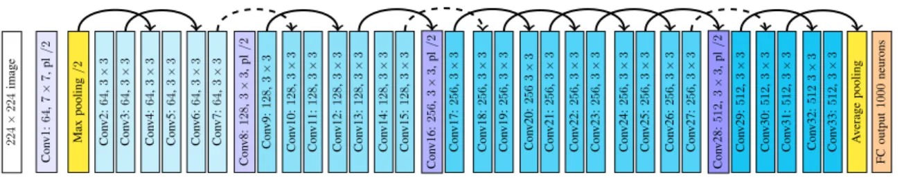
– AlexNet [6]: was the champion model in ImageNet Challenge 2012. With∼60million parameters and 650000 neurons, AlexNet was originally designed in two branches allowing parallel processing. It uses Local Response normalization, maxpooling with overlapping (window size 3, stride 2), a batch size of 128 examples, momentum of 0.9 weight decay of 0.0005. They initialized the weights using Gaussian-distributed random values with fixed σ = 0.01, and bias to 1 for the 2nd, 4th and 5th convolutional layers, and bias to 0 for the remaining layers. The learning rate was initialized to 0.01 and arbitrarily dividing this learning rate by 10 three times during the training stage. In Figure 5 we show a diagram of the layers and compare it with the VGG-16, the latter is described next.

– VGG-Net [22]: this architecture was developed to increase the depth while making all filters with at most 3×3 size. The rationale behind this is that 2 consecutive 3×3 conv. layers will have an effective receptive field of 5×5, and 3 of such layers an effective receptive field of 7×7when combining the feature maps. The authors claim that stacking 3 conv. layers with 3×3 filters instead of using just one with filter size 7×7 has the advantage of incorporating more rectification layers, making the decision function more discriminative. Also, it incorporates 1×1 conv. layers that perform a linear projection of a position (x, y) across all feature maps in a given layer. There are two most commonly used versions of this CNN: VGG-16 and VGG-19, respectively with 16 weight layers and 19 weight layers. In Figure 5 we show a diagram of the layers of VGG-16 and compare it with the AlexNet.

(9)

AlexNet architecture

224×224image Conv1:96filters11×11 Maxpooling1 Conv2:256filters5×5 Maxpooling2 Conv3:384filters3×3 Conv4:385filters3×3 Conv5:256filters3×3 Maxpooling3 FC14096neurons FC24096neurons FC3output1000neurons

224×224image Conv1:64filters3×3 Conv2:64filters3×3 Maxpooling1 Conv3:128filters3×3 Conv4:128filters3×3 Maxpooling2 Conv5:256filters3×3 Conv6:256filters3×3 Conv7:256filters1×1 Maxpooling3 Conv8:512filters3×3 Conv9:512filters3×3 Conv10:512filters1×1 Maxpooling4 Conv11:512filters3×3 Conv12:512filters3×3 Conv13:512filters1×1 Maxpooling5 FC14096neurons FC24096neurons FC3output1000neurons

VGG-16 architecture

Figure 5. Outline of CNN architectures: AlexNet with variable filter sizes (top), and VGG-16 with fixed3×3filter sizes (bottom).

During training, the batch size used is 256. LRN is not used since it shows no classification improvement but increased running time. Maxpooling uses window size 2 and stride 2. Training was regularized by weight decay using L2 regularization λ = 0.0005, and dropout with 0.5 ratio for the first two FC layers. Learning rate and initialization were similar to those used in AlexNet, but all bias parameters were set to 0 and an initialization followed also a pretraining approach.

– Residual Networks (ResNet) [23]: the study describ- ing ResNets raises the question of whether we really get better networks by simply stacking more layers. At the time of the publication VGG-19 was considered “very deep”, and the authors show that, although depth seems to be correlated with better results, in practice, when increasing the number of layers, the accuracy first saturates and then starts to degrade rapidly and fail to even work in the training set, therefore underfitting.

He et al. [23] claim that this could, in fact, be an optimization problem, and propose the use of residual blocks for networks with 34 to 152 layers. Those blocks are designed to preserve the characteristics of the original vector x before its transformation by some layer f_l(x) by skipping weight layers and performing the sum f_l(x) +x.

In Figure 6 we show a diagram of three different versions of such blocks, and in Figure 7 the ResNet architecture with 34 layers that uses the residual block and residual block with pooling. The authors claim that, because the gradient is an additive term, it is unlikely to vanish even with many layers. Interestingly, this architecture does not contain any FC hidden layers. After the last convolution layer, an Average pooling is computed followed by the output layer.

The bottleneck blocks (Figure 6-(c)) are designed to compress the depth of the input feature map via 1 ×1

x

weights

weights f(x)

+

f(x) +x

ReLU

identity

x

weights + pooling

weights f(x)

+

f(x) +p(x)

ReLU

pooling

xwithd= 256

64,1×1

64,3×3

256,1×1

f(x) +

f(x) +x

ReLU

(a) residual block (b) with pooling (c) bottleneck Figure 6. Modules to preserve the characteristics the original vector (identity) allows the vector to skip weight layers, typically skipping 2 layers:

(a) the original vectorxbefore its modification by weights is summed with its transformed versionf(x); (b) when some layer also include pooling operation, the dashed line indicates the original vector needed pooling to be summed; (c) in the bottleneck module illustrated, the depth (256) of the input is reduced by the first1×1layer of 64 filters and then restored back to 256 by the third layer.

convolutions with a reduced number of filters, and then restore its depth by adding another layer of containing a number of filters1×1equal to the depth of the input feature map. The bottleneck blocks are used in ResNet with 50, 101 and 152 layers. For example, the ResNet-50 is basically the ResNet-34 replacing all residual blocks (each containing 2 weight layers) with bottleneck blocks (each has 3 weight layers).

For the ImageNet training the authors adopt only Batch Normalization (BN) without regularization, dropout or normalization; data augmentation was performed using crops, horizontal flip and Fancy PCA; they also preprocessed the images by average subtraction. The batch size used was 256 and the remaining parameters are similar to the previously described methods as shown in Table I.

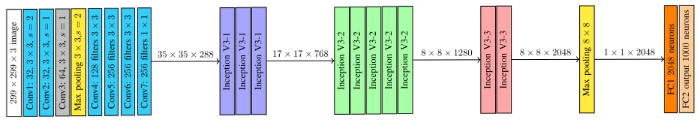
– GoogLeNet [24] and Inception [42]: the GoogLeNet as proposed by [24] and the VGGNet [22] achieved similar performances in the 2014 ImageNet challenge [2]. However, the GoogLeNet received attention due to its architecture based on modules called Inception (see Figure 8). Later improvements in this model are called Inception architectures such as the Inception V3 presented by [42], in which the authors also discuss design principles of CNN architectures including: (i) gentle decrease of representation size from input to output; (ii) use of higher dimensional representations per layer (and consequently more activation maps); (iii) use of lower dimensional embeddings using 1×1convolutions before spatial convolutions; (iv) balance of width (number of filters per layer) and depth (number of layers).

Recently, the same authors incorporated ideas from ResNets, producing many variants including Inception V4 and Inception-ResNet [45]. Here, for didactic purposes, we

(10)

224×224image Conv1:64,7×7,pl/2 Maxpooling/2 Conv2:64,3×3 Conv3:64,3×3 Conv4:64,3×3 Conv5:64,3×3 Conv6:64,3×3 Conv7:64,3×3 Conv8:128,3×3,pl/2 Conv9:128,3×3 Conv10:128,3×3 Conv11:128,3×3 Conv12:128,3×3 Conv13:128,3×3 Conv14:128,3×3 Conv15:128,3×3 Conv16:256,3×3,pl/2 Conv17:256,3×3 Conv18:256,3×3 Conv19:256,3×3 Conv20:2563×3 Conv21:256,3×3 Conv22:256,3×3 Conv23:256,3×3 Conv24:256,3×3 Conv25:256,3×3 Conv26:256,3×3 Conv27:256,3×3 Conv28:512,3×3,pl/2 Conv29:512,3×3 Conv30:512,3×3 Conv31:512,3×3 Conv32:5123×3 Conv33:512,3×3 Averagepooling FCoutput1000neurons

Figure 7. Outline of ResNet-34 architecture. Solid lines indicate identity mappings skipping layers, while dashed lines indicate identity mappings with pooling in order to match the size of the representation in the layer it skips to.

x

1×1

5×5

1×1

3×3

Pool

1×1

Feature maps concatenation

x

1×1

3×3

1×1

3×3

Pool

1×1

(a) Original Inception (b) Inception v3-1

x

1×1

1×k

k×1

1×k

k×1

1×1

1×k

k×1

Pool

1×1

x

1×1

3×3

1×3 3×1

1×1

1×3 1×3

Pool

1×1

(c) Inception v3-2 (d) Inception v3-3 Figure 8. Inception modules (a) traditional; (b) replacing the5×5 by two3×3convolutions; (c) with factorization ofk×kconvolution filters, (d) with expanded filter bank outputs.

focus on Inception V3 since the V4 is basically a variant of the previous one.

The Inception module breaks larger filters (e.g. 5×5, 7 × 7) that are computationally expensive, into smaller consecutive filters that have the same effective receptive field. Note that this idea was already explored in VG- GNet. However, the Inception explores this idea stacking different sequences (in parallel) of small convolutions and concatenates the outputs of the different parallel sequences.

The original Inception [24] is shown in Figure 8-(a), while in Inception V3 it follows the design principle (iii) and

proposes to factorize a 5×5 convolution into two 3×3 as in Figure 8-(b). In addition, two other modules are proposed: a factorization module for k×k convolutions as in Figure 8-(c), and an expanded filter bank to increase the dimensionality of representations as shown in Figure 8-(d).

We show the Inception V3 architecture in Figure 9: the first layers include regular convolution layers and pooling, followed by different Inception modules (type V3-1,2,3). We highlight the size of the representation in some transitions of the network. This is important because to show that while the first two dimensions shrink, the third increases following the principles (i), (ii) and (iv). Note that the Inception modules type V3-2 are used with size k= 7 for an input representation of spatial size17×17. The Inception modules type V3-3, that output a concatenation of 6 feature maps per module has the intention of increasing the depth of the feature maps in a coarser scale (spatial size 8×8).

Although this architecture has 42 layers (considering internal convolutions layers inside Inception modules), because of the factorization is has a small size in terms of parameters.

For Inception V3 the authors also employ a label- smoothing regularization (LSR) that tries to constrain the last layer to output a non-sparse solution. Given an input example, let k be the index for all classes of a given problem, Y(k) be the ground truth for each classk,Yˆ(k) the predicted output and P(k) a prior for each class. The LSR can be seen as using a pair of cross-entropy losses, one that penalizes the incorrect label, and a second that penalizes it to deviate from the prior label distribution, i.e.

(1−γ)`(Y(k),Yˆ(k)) +γ`(P(k),Yˆ(k)). The parameterγ controls the influence of the LSR andP represent the prior of a given class.

To train the network for ImageNet, they used LSR with a uniform prior, i.e. the same for all classes: P(k) = 1/1000∀k for the ImageNet 1000-class problem and γ = 0.1, BN is applied in both convolutional and FC layers.

The optimization algorithm is the RMSProp. All other parameters are standard. They also used gradient clipping with threshold 2.

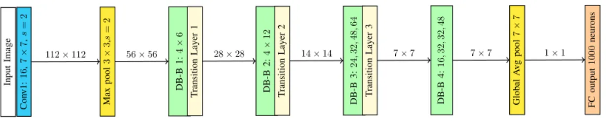
– DenseNet [25]: inspired by ideas from both ResNets and Inception, the DenseNet introduces the DenseBlock, a sequence of layers where each layer l takes as input

(11)

299×299×3image Conv1:32,3×3,s=2 Conv2:32,3×3,s=1 Conv3:64,3×3,s=1 Maxpooling3×3,s=2 Conv4:128filters3×3 Conv5:256filters3×3 Conv6:256filters3×3 Conv7:256filters1×1 InceptionV3-1 InceptionV3-1 InceptionV3-1 InceptionV3-2 InceptionV3-2 InceptionV3-2 InceptionV3-2 InceptionV3-2 InceptionV3-3 InceptionV3-3 Maxpooling8×8 FC12048neurons FC2output1000neurons

35×35×288 17×17×768 8×8×1280 8×8×2048 1×1×2048

Figure 9. Outline of Inception V3 architecture. Convolutions do not use zero-padding except for Conv3 (in gray). The stride is indicated bys. We highlight the size of the representations before and after the Inception modules types, and also after the last max pooling layer.

all preceding feature maps x1,x2,· · · ,xl−1 concatenated.

Thus, each layer produces an output which is a function of all previous feature maps, i.e.:

xl=Hl([x1,x2,· · ·,xl−1]).

Hence, while regular networks with L layers have L connections, each DenseBlock (illustrated in Figure 10) has a number of connections following an arithmetic progression, i.e. ^L(L+1)₂ direct connections. The DenseNet is a concatenation of multiple inputs ofHl()into a single tensor. Each Hl is composed of three operations, in sequence: batch normalization (BN), followed by ReLU and then a 3×3 convolution. This unusual sequence of operations is called pre-activation unit, was introduced by He et al. [27] and has the property of yielding a simplified derivative for each unit that is unlikely to be canceled out, which would in turn improves the convergence process.

Transition layers are layers between DenseBlocks composed of BN, a 1×1 Conv.Layer, followed by a 2×2 average pooling with stride 2.

Variations of DenseBlocks: they also experimented using bottleneck layers, in this case each DenseBlock is a sequence of operations: BN, ReLU, 1×1 Conv., followed by BN, ReLU, 3×3 Conv. This variation is called DenseNet-B.

Finally, a compression method is also proposed to reduce the number of feature maps at transition layers with a factorθ.

When bottleneck and compression are combined they refer the model as DenseNet-BC.

Each layer has many input feature maps; if each Hl

produceskfeature maps, then thel^thlayer hask0+k×(l−1) input maps, where k0 is the number of channels in the input image. However, the authors claim that DenseNet requires fewer filters per layer [25]. The number filters k is a hyperparameter defined in DenseNet as thegrowth rate.

For the ImageNet dataset k = 32 is used. We show the outline of the DenseNet architecture used for ImageNet in Figure 11.

– Comparison and other archictectures: in order to show an overall comparison of all architectures described, we listed the training parameters, size of the model and top1 error in the ImageNet dataset for AlexNet, VGGNet, ResNet, Inception V3 and DenseNet in Table I.

Input BN+ReLU+Conv:H1 BN+ReLU+Conv:H2 BN+ReLU+Conv:H3 BN+ReLU+Conv:H4 BN+ReLU+Conv:H5 Transition(BN+Conv+Pool)

Figure 10. Illustration of a DenseBlock with 5 functions H_l and a Transition Layer.

Finally, we want to refer to another model that was designed to be small, compressing the representations, the SqueezeNet [46], based on AlexNet but with 50× fewer parameters and additional compression so that it could, for example, be implemented in embedded systems.

L. Beyond Classification: fine-tuning, feature extraction and transfer learning

When one needs to work with a small dataset of images, it is not viable to train a Deep Network from scratch, with randomly initialized weights. This is due to the high number of parameters and layers, requiring millions of images, plus data augmentation. However, models such as the ones described in this paper (e.g. VGGNet, ResNet, Inception), that were trained with large datasets such as the ImageNet, can be useful even for tasks other than classifying the images from that dataset. This is because the learned weights can be meaningful for other datasets, even from a different domain such as medical imaging [47].

In this context, by starting with some model pre-trained with a large dataset, we can use the networks as Feature Extractors[48] or even to achieveTransfer Learning[49].

It is also possible to perform Fine-tuning of a pre-trained model to create a new classifier with a different set of

(12)

InputImage Conv1:16,7×7,s=2 Maxpool3×3,s=2 DB-B1:4×6 TransitionLayer1 DB-B2:4×12 TransitionLayer2 DB-B3:24,32,48,64 TransitionLayer3 DB-B4:16,32,32,48 GlobalAvgpool7×7 FCoutput1000neurons

112×112 56×56 28×28 14×14 7×7 7×7 1×1

Figure 11. Outline of DenseNet used for ImageNet. The growth rate isk= 32, each Conv.layer corresponds to BN-ReLU-Conv(1×1) + BN-ReLU- Conv(3×3). A DenseBlock (DB)4×6means there are 4 internal layers with 6 filters each. The arrows indicate the size of the representation between layers.

Table I

COMPARISON OFCNNMODELS IN TERMS OF THE PARAMETERS USED TO TRAIN WITH THEIMAGENET DATASET(INCLUDING AND THEIR

ARCHITECTURES

Training Parameters Model ImageNet

CNN Batch size Learn.rate Optm.alg. Optm.param. Epochs Regularization # Layers Size top-1 error

AlexNet 128 0.01 SGD α= 0.9 90 Dropout 8 240MB 37.5%

VGGNet 256 0.01 SGD α= 0.9 74 L2 + Dropout 16-19 574MB (19 lay.) 24.4%

ResNet 256 0.1 SGD α= 0.9 120 BN 34-152 102MB (50 lay.) 19.3%

Inception V3 32 0.045 RMSP α, γ= 0.9 100 BN + LSR 42 96MB 18.7%

DenseNet 128 0.1 SGD α= 0.9 100 BN 40-250 30MB (161 lay.) ∼18.7%

classes.

In order to perform the aforementioned tasks, there are many options that involve freezing layers (not allowing them to change), discarding layers, including new layers, etc. As we describe next for each case.

– Building a new CNN classifier via Fine-Tuning: it is likely that a new dataset has different classes when compared with the dataset originally used to train the model (e.g the 1000-class ImageNet dataset). Thus, if we want to create a CNN classifier for our new dataset based on a pre-trained model, we have to build a new output layer with the number of neurons equal to the number of classes. We then design a training set using examples from our new dataset and use them to adjust the weights of our new output layer.

There are different options involving fine-tuning, for example: (i) allow the weights from all layers to be fine-tuned with the new dataset (not only the last layer), (ii) freeze some of the layers, and allow just a subset of layers to change, (iii) create new layers randomly initialized, replacing the original ones. The strategy will depend on the scenario. Usually, the approach (ii) is the most common, freezing the first layers, but allowing weights of deeper layers to adapt.

– CNN-based Feature Extractor: in this scenario, it is possible to make use of pre-trained CNNs even when the dataset is composed of unlabelled (e.g. in clustering problems) or only partially labelled examples (e.g. in anomaly detection problems), in which without label information it is not possible to fine-tuning the weights [50].

In order to extract features a common approach is to perform a forward pass with the images and then use the feature/activation maps of some arbitrary layer as features [48].

For example, using an Inception V3 network, one could get the1×1×2048output from the last Max Pooling layer (see

Figure 9), ignoring the output layer. This set of values can be seen as a feature vector with 2048 dimensions to be an input for another classifier, such as the SVM for example.

If a more compact representation is needed, one can use dimensionality reduction methods or quantization based on PCA [51] or Product Quantization [52], [53].

– CNN as a building block: pre-trained networks can also work as a part of a larger architecture. For example in [54] pre-trained networks for both photo and sketch images are used to compose a triplet network. We discuss those type of architectures in Section VI.

IV. AUTOENCODERS(AES)

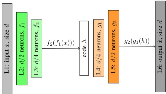
An AE is a neural network that aims to learn to approximate an identity function. In other words, when we feed an AE with a training example x it tries to generate and outputxˆ that is as similar as possible to x. At first glance, it may seem like such task is trivial: what would be the utility of the AE if it just tries to learn the same data we already have as input? In fact, we are not exactly interested in the output itself, but rather on the representations learned in other layers of the network. This is because the AEs are designed in such way that they are not able to learn a dumb copy function. Instead, they often discover useful intrinsic data properties.

From an architectural point of view, an AE can be divided into two parts: an encoderf and a decoderg. The former takes the original input and creates a restricted (more compact) representation of it – we call this representation code. Then, the latter takes this code and tries to reconstruct the original input from it (See Figure 12).

Because the code is a limited data representation, an AE cannot learn how to perfectly copy its input. Instead,