Research Collection
Working Paper
Regional Borders, Commuting and Transport Network Integration
Author(s):
Loumeau, Gabriel Publication Date:
2020-12
Permanent Link:
https://doi.org/10.3929/ethz-b-000458728
Rights / License:
In Copyright - Non-Commercial Use Permitted
This page was generated automatically upon download from the ETH Zurich Research Collection. For more information please consult the Terms of use.
KOF Working Papers, No. 489, December 2020
Regional Borders, Commuting and Transport Network Integration
Gabriel Loumeau
ETH Zurich
KOF Swiss Economic Institute LEE G 116
Leonhardstrasse 21 8092 Zurich, Switzerland Phone +41 44 632 42 39 Fax +41 44 632 12 18 www.kof.ethz.ch kof@kof.ethz.ch
Regional Borders, Commuting and Transport Network Integration
Gabriel Loumeau∗ ETH Zürich
December 27, 2020
Abstract
I study how and why economic activity varies around regional borders. Spatial quasi-experimental variation around French departmental borders reveals discontinuous commuting and residential patterns. To tackle the endogenous border placement problem, I exploit a geometric border design proposed during the French Revolution. I then calibrate a spatial quantifiable general equilibrium framework to structurally match the quasi-experimental estimates. The commuting and residential discontinuities are well explained by a 7km bilateral distance penalty when crossing regional borders, which is the consequence of the decentralized planning and development of local transport networks. Policy simulation shows that integrating local transport networks leads to a 11.7% average growth in real per capita residential income.
Keywords: Border, Commuting, Discontinuity, Transport network, Decentralization.
JEL classification: R12, R42, O18.
∗I am grateful to seminar and workshop participants in Paris, Dijon and Bern. In particular, I thank (in alphabetical order) Marie Brueillé, Peter Egger, Maximilian von Ehrlich, Miren Lafourcade, Nicole Loumeau, José de Sousa, Florence Puech, Christian Stettler, Clémence Tricaud and Lionel Védrine for helpful comments and suggestions.
Email address: loumeau@ethz.ch.
1 Introduction
With 9.7 million kilometers in length defining 49,572 jurisdictions worldwide, regional borders are one of the most common features of today’s economic geography.1 Typically operating in ho- mogeneous socio-economic environments without border controls, these borders are barely visible to the millions of daily cross-border commuters (in the U.S., Germany and France alone, 13.5 million commuters cross regional borders).2 Yet, regional borders delineate jurisdictions which are often sole responsible for the development of local transport networks – a setting which does not guarantee local network integration. Given the well-established role of transport networks in shaping regional economic geographies, such borders may then be less innocuous than first thought.3 Any spatial mismatch in local networks may lead to large costs for the economy as a whole. For instance, frictions at regional borders are likely to affect the benefits of commuting openness for local labor markets (Monte, Redding, and Rossi-Hansberg,2018), or likely to induce large opportunity costs when considering a value of time associated with commuting in the range of $20 to $40 an hour (Brownstone and Small,2005).
Using spatial quasi-experimental variation around French departmental borders, this paper establishes robust evidence that commuting flows, labor catchment areas and local residential masses vary discontinuously at regional borders. To tackle the problem of endogenous border placement, I exploit a geometric border design proposed during the French Revolution. Then, combining a structural framework to the natural border experiment, the paper shows that the observed discontinuities at regional borders can be explained by the non-integration of local transport networks – a consequence of their decentralized planning and development. Finally, simulation results indicate that integrating such transport networks likely leads to large average real income gains.
The empirical analysis starts by using a spatial regression discontinuity (RD) estimator on municipal data to document commuting and residential location choice patterns around regional borders (see, among others,Hahn, Todd, and der Klaauw,2001;Lee and Lemieux,2010;Calonico, Cattaneo, and Titiunik, 2014; Ehrlich and Seidel,2018). Comparing a municipality at a regional border to its neighbor on the other side of the border, I estimate a discontinuity in the likelihood to commute across the border of 65 percentage points (using both parametric and non-parametric
1In this paper, I consider as regional, all administrative borders between the national and the municipal levels (e.g, US States, European NUTS2 and NUTS3 regions, Chinese Provinces and Prefectures, etc.). Source: Authors’
own calculation based on the 2019 Database of Global Administrative Areas (GADM). See: https://gadm.org/.
2Source: 5.3 millions across US State borders, Census Bureau, 2011; 3.6 million across Länder borders, Region- aldatenbank, 2018; 4.6 million across Département borders, INSEE, 2010.
3See, among others, Baum-Snow (2007); Duranton and Turner (2012); Faber (2014); Tombe and Zhu (2015);
Fretz, Parchet, and Robert-Nicoud(2017);Caliendo, Parro, Rossi-Hansberg, and Sarte(2018).
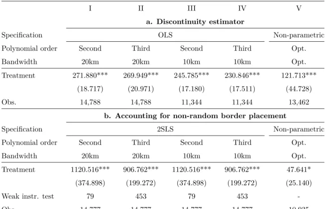
approaches). This naturally impacts the labor catchment possibilities of jurisdictions with large labor markets. On average, the number of workers commuting to regions with large labor markets drops discontinuously by 121 at the border. I further show that residential density also jumps at regional borders. Municipalities at regional borders on the side with the larger labor market display an average excess residential mass of 79 residents (equivalent to 10.2% of the average local population).4
To control for endogenous border placement – an issue often over-looked in the spatial bor- der literature – I exploit a geometric border plan proposed during the French Revolution which inspired the final design of French departmental borders. The geometric design was proposed by the Sieyès committee in 1789, and recommended to divide the country geometrically into 81 equal sized departments (squares of 18 league per side, approx. 100km). I use the distance to the regional border under the geometric delineation in an Instrumental Variable (IV) approach to predict the distance to the observed regional border. The results are qualitatively similar when using the standard and the IV spatial RD estimators.
I hypothesize that the lack of integration of local transport networks explains the commuting and residential discontinuities observed at regional borders. In France, 71% of all road kilome- ters are administered at the department level, and no institutional setting insures the proper integration of transport networks. To test this hypothesis, I first show – parametrically and non-parametrically – that travel distance on the road network to the centroid of a regional ju- risdiction drops discontinuously at the border. Reaching the centroid of a department takes on average 7km more when starting just on the other side of the border, as opposed to just inside the jurisdiction.5 I further test for the spatial distribution of other local public services which are departmental prerogatives (i.e., secondary schools and fire departments). I also test for variation in travel distances around local borders which are not associated with local transport network provision (i.e., Functional Urban Areas).6 Overall, these additional analyses support the hypoth- esis that the decentralized provision of transport networks is, at least, a major determinant of the discontinuous commuting and residential patterns observed.
Furthermore, I test whether a 7km discontinuity alone in travel distances is sufficient to ratio- nalize the commuting and residential discontinuities observed. To do so, I structurally estimate commuting and residential density patterns in a spatial quantifiable general equilibrium framework à la Monte et al. (2018). I use the results from the spatial regression discontinuity estimator as moments in a Generalized Method of Moments (GMM) approach. This structural approach con-
4The average municipality within 10km of a departmental border hosts 779 residents (see descriptive statistics in Table7, AppendixA).
5Bandwidths of 500m and 1km are used.
6Functional Urban Areas (FUA) are the European equivalent of the US Metropolitan Statistical Areas (MSA).
firms that a 7km distance penalty when crossing regional borders best explains the discontinuities observed.
Finally, I study the cost and benefits of integrating local road networks using a spatial quan- tifiable general equilibrium framework à laMonte et al.(2018). As in the new economic geography literature, the framework supposes gains from agglomeration that arise from the love of varieties and increasing returns to scale. I complement the framework with two key ingredients. First, I suppose a central institution in charge of integrating local transport networks. Costs of integration are financed by a nation-wide head tax levied on all workers. Such non-distortionary tax setting allows (i) a direct exogenous matching from a tax rate to an increased local transport network integration, and (ii) the possible redistribution of the policy gains in an intuitive manner. Second, in line with the residential discontinuity estimator, I introduce a mechanism under which available residential floor space is endogenously determined by local residential income. Using precise geo- localized data on commutes, residential and workplace densities, and local transport networks, I complete the calibration of the model to match the main characteristics of the French economic geography in 2010. I then use this framework to run a cost-benefit analysis of integrating the local transport networks. Policy simulation results indicate that removing the penalty leads to a 11.7% average growth in local residential income. Especially, residential per capita real income at the wide periphery of Paris’ metropolitan area, as well as local workplace income within this metropolitan area, increase.
The remainder of this paper is organized as follows. After discussing the related literature in Section 2, I present the institutional background and descriptive evidence in Sections 3 and 4, respectively. Before documenting commuting and residential location choice patterns around local borders using quasi-experimental estimators in Section6, I detail the theoretical framework in Section 5. I study how decentralization affects cross-border travel distances in Section 7. In Section8, I simulate the integration of regional transport networks, and analyze its consequences on the French economic geography. Finally, Section 9concludes.
2 Literature
The study of discontinuous effects at national and regional borders is not new. A vast literature has shown that national borders act as spatial barrier to various economic outcomes.7 The border
7I distinguish this literature from a second stand of the literature that has used borders as an exogenous source of policy variation in space. For instance,Dube, Lester, and Reich(2010) exploit differences in minimum wage levels across US State border to study their effects on earnings and employment. Kumar(2018) looks at Texas’s interstate borders to study how limitations on home equity borrowing affect the likelihood of mortgage default. Egger and Lassmann (2015), Erhardt and Haenni (2018), and Eugster and Parchet (2019) exploit language differences at
puzzle literature in international trade highlights the presence of a border effect in trade flows at national borders (McCallum, 1995; Obstfeld and Rogoff, 2001; Anderson and van Wincoop, 2003; Evans, 2003). Ahlfeldt, Redding, Sturm, and Wolf (2015) show how the Berlin wall acted as a barrier to agglomeration and dispersion forces. Beerli, Ruffner, Siegenthaler, and Peri (2018) document the effect of opening a national border to cross-border commuting on labor market characteristics. Pinkovskiy (2017) reveals discontinuities in growth rates at national borders.
The literature has also looked at within-country border effects. Courant and Deardorff (1992) highlight the role of within country trade as a determinant of international trade patterns. Wrona (2018) reveals the presence of an intranational border effect on trade flows using regional Japanese data. Using municipal merger reforms in Germany,Egger, Koethenbuerger, and Loumeau (2017) study how the removal of local borders concentrates economic activity locally. Felbermayr and Tarasov(2015) model the spatial provision of transport infrastructure around inter- and intrana- tional borders by non-cooperative governments, and highlight how underprovision of infrastruc- ture may contribute to solve the trade border puzzle. Combes, Lafourcade, and Mayer (2005) emphasize the role of networks across administrative borders as determinants of trade flows.
Relative to the inter- and intranational border literature, the present paper innovates in three respects. First, it is the first to provide quasi-experimental evidence of a non-trade border effect at the intranational level (i.e., even under common language, taxes, social norms, etc). Second, the estimation of the travel distance gap at regional borders induced by the decentralized provision of transport infrastructure is novel. Third, this paper offers an Instrumental Variable (IV) strategy based on a unique historical setting to account for possible non-random border placement, an issue that has mostly been ignored in previous research.
This paper also relates to the emerging literature applying research methodologies that com- bine structural quantitative techniques with quasi-random policy variations. Ahlfeldt et al.(2015) exploit the construction and the fall of the Berlin Wall as a source of exogenous variation to in- form a quantifiable urban general equilibrium model. Chen, Liu, Suárez Serrato, and Xu (2018) combine quasi-experimental variation around notches and structural estimation to capture the complex effects of tax cuts on R&D investments in China.
Moreover, this paper relates to the literature on endogenous transport infrastructure around borders. Felbermayr and Tarasov (2015) study under-investment in transport networks around
Swiss cantonal borders to understand the role of culture and preferences in shaping nowadays economic geography.
Using the fall of the Iron Curtain,Ehrlich and Seidel(2018) analyze the persistence effects of place-based policies.
Holmes(1998) andRohlin, Rosenthal, and Ross(2014) use cross-border variations to study firm location decisions.
Coomes and Hoyt (2008) focus on tax evasion and avoidance, whereas Agrawal(2015) analyze tax competition across US State borders. Agrawal and Hoyt(2018) exploit tax differentials at US State borders within metropolitan areas to analyze the effect of local taxes on commuting patterns, and ultimately on welfare.
borders as national governments do not internalize the benefits from reductions in domestic trans- portation costs that accrue to foreign consumers. Sippel, Nolte, Maarfield, Wolff, and Roux(2018) andChristmann, Mostert, Wilmotte, Lambotte, and Cools(2020) present case studies investigat- ing possible missing cross-border connections between European countries.
Additionally, this paper contributes to the urban economics literature highlighting the role of commuting in determining urban equilibrium characteristics,8 by offering a natural experiment to further understand how commuting affects the location and growth of economic activity. This paper shows that transport network decentralization leads to regional borders acting as a barrier to commuting (by increasing the distance and duration of commutes), which, in turn, affects regional workplace employment, as well as residential location choices.
Finally, this paper relates to the literature on inefficiencies arising from decentralization. Fol- lowing early works by Tiebout (1956) and Oates (1969), the local public finance literature has long argued in favor of decentralization as it allows individuals to “vote with their feet” and leads to more efficient local public finances. However, more recent studies have questioned the effi- ciency of a decentralized organization. For instance, given mobile and heterogeneous households, Calabrese, Epple, and Romano (2012) show that inefficiencies arising from decentralization and property taxation are substantial. Beyond the public finance literature, the experimental liter- ature (e.g., van Huyck, Battalio, and Beil, 1990, 1991) highlights the inefficiencies arising from failure to coordinate among economic agents. Applying this framework to regional jurisdictions under a decentralized organization appears natural and helps rationalize the discontinuities in travel distances at regional borders observed in this paper.
3 Three facts about French departments
The current French administrative division is composed of three layers below the national one: 13 regions, 101 departments (including overseas), and 34,968 municipalities (as of March 2019). This paper focuses on the second administrative layer in mainland France. To study the regional border effect carefully, French departments offer three key advantages. First, their design was inspired by a geometric delineation of the country into 81 equal sized squares of 100km sides. Second, in most cases, departmental borders do not follow natural features such as rivers, mountains, etc.
Finally, departments have little public finance autonomy. On the revenue side, more than 80%
of their income is exogenously allocated by the central government. On the expenditure side, the level of service and benefit provision is subject to extensive mandates which strongly restrict – if
8See, among others, Alonso(1964);Mills(1967);Muth(1969);Lucas and Rossi-Hansberg(2002);Desmet and Rossi-Hansberg(2013);Behrens, Mion, Murata, and Suedekum(2017);Monte et al.(2018).
not, eliminate – regional differences. In what follows, I explain the mentioned advantages in more detail.
3.1 Fact 1: Inspired by an historical geometric border design proposal
French departments were created during the French Revolution. Before the Revolution, the French administrative division into provinces was particularly complex. Provinces differed greatly in size, administrative borders were not all precisely defined, and did not always match with local fiscal, religious or military jurisdictions. Consequently, in 1789, the newly created National Assembly decided to reform the national administrative division. A committee, lead by the abbé Sieyès, was formed to propose a partition of France into regional units. The committee recommended to divide the country geometrically into 81 equal sized departments (squares with sides of 18 league, approximately 100km, except for those cut by national boundaries). Each department was then to be further divided into nine equal sized units, which would again be divided into nine equal sized units. Given that the French population was mostly rural at the time, these last sub-units were expected to be of similar population size. Figure 1 displays a scan of the historical map defining this geometric division.9
Inspired by the geometric proposal, the division finally adopted by the assembly in 1790 kept the goal of partitioning the country into equal sized units, but departed from the pure geometrical approach.10 The final size was chosen such that one could reach the departmental capital from any point on the border within 24 hours (by horse). Except for regions impacted by the evolution of France’s territory over time, the division has barely changed until today. Figure14(Appendix B) shows the departmental borders as they are since 1964.
3.2 Fact 2: Limited overlap with natural features
A key concern when analyzing effects of regional borders is the possible overlap between border placement and natural features. Commuting across a border might be less likely, not because of a border per se, but because a natural feature makes it harder to cross the border. On this issue, the French case is particularly interesting to study. As mentioned above, the French National Assembly decided to design departmental jurisdictions such that they would all have a similar size and shape. This imposed strong limitations on border placement. Consequently, apart from a few exceptions (e.g., the Rhône in the South-East), departmental borders do not follow France’s
9The absence of Corsica in the geometric division motivates the focus on mainland France in this paper.
10Figure 14 (Appendix B) shows the final departmental division adopted by the French National Assembly in 1790.
Figure 1: Geometric proposal by the Sieyès committee in 1789
Notes: Large green/white squares with sides of 18 league, approximately 100km, represent the proposed departmental division.
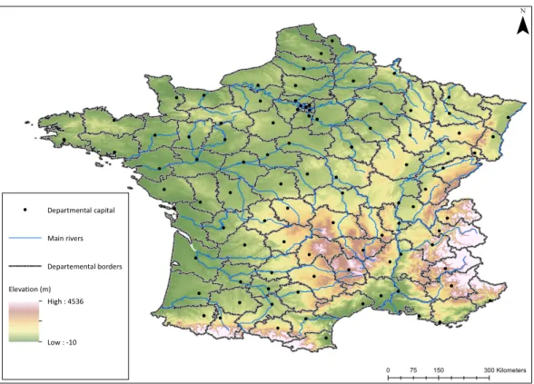
main natural features (i.e., main rivers and land elevation), as shown in Figure 2. To further control for non-endogenous border placement, I use the geometric proposal in an IV approach as detailed in Section 6. I also run robustness tests excluding all bilateral connection paths within 20km of a natural feature (i.e., river or mountain), a strategy also adopted in Black (1999) and Ehrlich and Seidel (2018). Overall, natural features appear to have little impact on the results.
Furthermore, the requirement that the local capital could be reached within one day by horse from any point in the department forced capitals to be centrally located within each jurisdiction, as shown in Figure 2. Hence, the special case of having capital cities located directly at regional border – which could be a source of bias when looking at economic activity close to regional borders – is a minor issue, if at all, in the present context.
3.3 Fact 3: Limited public finance autonomy
Departments are legally required to run a balanced budget, i.e., total revenues equal total spend- ing. I retain this characteristic when modeling regional spending in Section 5. Based on the
Figure 2: Departmental borders and natural features
Departmental capital Main rivers
Departemental borders Elevation (m)
High : 4536
Low : -10
0 75 150 300Kilometers
¯
2016 official departmental budget data, Panel a of Table8(Appendix B) shows the departmental revenues, which come from mostly three sources in similar proportions: local taxes, transfers, and tax transfers. Out of the three, departments are only able to influence revenues from local taxes, mostly via the local land value tax which represent a little less than 20% of their total revenues.
Overall, the rate of the local land value tax is inversely related to the tax base, i.e., the hypo- thetical rental value. Hence, even though local differences in the per capita amount paid do exist, these differences are minimal. To insure that local public finance differences across departments do not confound the results, I include border fixed effects in the analysis; hence, controlling for tax differentials at each border.11 No significant changes in the results are observed.
Furthermore, French departments are locally competent on mostly four items: social pro- grams, regional roads, secondary eduction and fire departments. The level of provision of each item is mandated by national rules. Hence, except for a more (or less) efficient administrative organization, departments have almost no leeway to influence these four items locally. Panel b of Table 8 (Appendix B) examines the total spending of the department using the 2016 official regional budget data. Social programs constitute the lion’s share, i.e., 65%, of the departmental spendings. Even though spending on the remaining categories represent between 4% and 7% of the total spending, the amounts of spending on this items are far from negligible (i.e., between
11I also run a robustness check including the local rental value per m2 to further account for differences in the tax base (Table9(Appendix B).
2.6 and 4.2 billion e). For instance, the total length of the road transport networks financed and administered by the departments constitute 71% of the sum of all road kilometers in France.
Aside from regional road networks, secondary schools and fire departments are the only public service administered by the departments which may affect residential location choices and com- muting flows. In the empirical exercise below, I test for a gap in fire stations, secondary schools and secondary pupil density around regional borders. Each of these outcomes appears to vary smoothly at regional borders. Moreover, note that given the use of border-specific fixed effects, any systematic difference in fire departments and secondary school characteristics is likely to be captured.
4 Descriptive evidence
After briefly describing the data used in this paper, this section provides descriptive evidence suggesting that regional borders affect surrounding economic activity.
Data
The data used in this paper come from the following sources.12 All demographic and administra- tive data are provided by the National Institute of Statistics and Economic Studies (INSEE) for the year 2010. All geolocalized data (adminitrative borders and transport networks) are provided by the National Institute of Geographic and Forest Information (IGN) as of 2015, and processed using the geographic information system ArcGIS (esp., ArcGIS Network Solver). The map of the geometric border proposal by the Sieyès committee is provided by French National Archives (AN). Lastly,Chapelle and Eyméoud (2017) provide housing rents at the municipal level.
Table 7, in the Appendix A, shows simple descriptive statistics for municipalities within dif- ferent bandwidths around local borders. Within 10km of a border, the average municipality hosts 779 residents and has an area of 16km2. The average median yearly income amounts to e19,811;
and housing rents are on average ofe9.27 per m2 and month. 89% of workers reside and work in the same regional jurisdiction.
Cross-border commuting
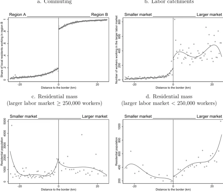
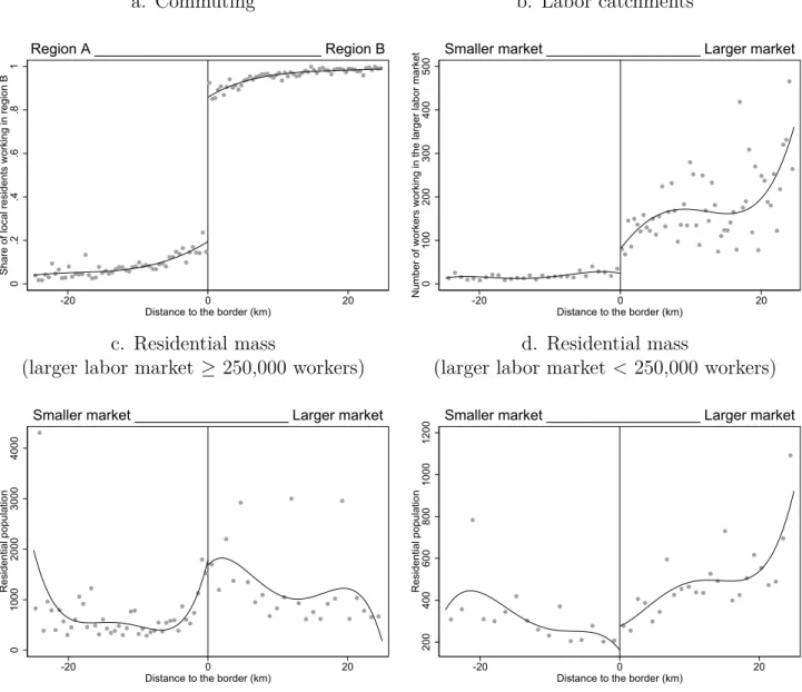
I start by describing commuting flows around regional borders. Conditional on a destination department – which I generically label region B – Figure 3 shows the average share of local residents commuting to region B around the regional borders. Averages are taken over 2km bins
12Section Aprovides an in depth description of the Data.
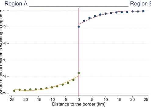
when considering all destination departments. The figure is based on the universe of residence- to-workplace commutes in France in 2010. The horizontal axis displays the great circle distance to the border in kilometers. The orientation is defined such that, without loss of generality, the destination jurisdiction is placed on the right side with positive distances to the border. Assuming homogeneous commuters – which is mostly verified in Section 6.4 – the share of local residents should capture well how local borders affect commuting flows. Absent any border effect, one would expect the two curves in Figure3tomeet at the border. Note that the precise meeting point may not be 50% as neighboring regions may be very different, e.g., in terms of labor market size.
However, a discontinuity of almost 60 percentage points is present at the border. This implies that workers disproportionately refrain from crossing the regional border, even when residing at the border.
Figure 3: Share of local residents by workplace location around regional borders
0.2.4.6.81Share of local residents working in region B
-25 -20 -15 -10 -5 0 5 10 15 20 25
Distance to the border (km)
Region A ________________________________ Region B
Notes: This graph is based on bilateral statistics using the universe of residence-to-workplace commutes in France in 2010. The average share of residence-to-workplace commutes by workplace location per km to the border is displayed. Scatters are obtained by
taking the average share within 2km bins. Predictions from linearly regressing the average share on distance and distance squared separately below and above the border are also reported. Finally, I use a 25km bandwidth.
Labor catchment areas
The observed discontinuity in commuting flows is likely to affect the labor catchment possibilities of large labor markets. Figure4displays the residential location of workers working in the region with the larger labor market. The size of a region’s labor market is defined as the sum of workers
working in the region. Locations within the region with the larger labor market are attributed positive distance to the border, whereas locations on the other side of the border are given negative distances. The vertical axis displays the average number of residents working in the larger labor market over 2km bins. As opposed to Figure 3, Figure 4 only considers one direction of cross- border commuting, i.e., towards the larger labor market. A sharp discontinuity appears at the border. The number of residents working in the larger labor market jumps by about 300 residents as one enters the regional with the larger labor market.13 Hence, the border seems to cut through the larger labor market’s catchment area.
Figure 4: Labor catchments around regional borders
0200400600Average local resident count
-25 -20 -15 -10 -5 0 5 10 15 20 25
Distance to the border (km)
Smaller market ______________________ Larger market
Notes: Bilateral statistics using the universe of residence-to-workplace commutes in France in 2010. Scatters are obtained by taking the average number of residents working in region B within 2km bins. Predictions from linearly regressing the average share on
distance and distance squared separately below and above the border are also reported. Finally, I use a 25km bandwidth.
Residential location choice
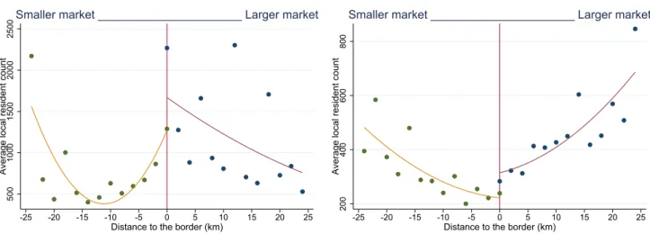
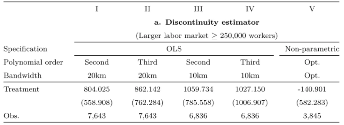
Intuitively, the discontinuity in labor catchment areas observed in Figure 4 may arise from dis- continuous commuting flows, but also due to an excess residential mass at the border on the side with the larger labor market. Figure 5 studies residential count around the border for different labor market sizes: borders around which the larger labor market is greater or equal to 250,000
13To properly compare residential count on both sides of a regional border, it is important to exclude mu- nicipalities close to national borders. In the present case, all locations within 30km of a national borders are excluded.
workers (Panel a),14 borders around which the larger labor market is less than 250,000 workers (Panel b). The rational for this distinction is that France’s larger urban areas extend beyond their department of origin, which is not the case when one considers smaller labor markets. As in Figure4, the horizontal axis displays the distance to the border with positive distances within the region with the larger labor market. On the vertical axis, I display the average resident count by bins of 5km. A discontinuity in average local resident count appears when looking at borders around which the larger labor market is less than 250,000 workers (Panel b). The discontinuity imprecisely observed in Panel a is driven by Paris outer districts (in French: “arrondissements”).
In Panel b, a discontinuity of about 150 residents is observed.
Figure 5: Residential location choice, labor market size and regional borders a. Larger labor market ≥ 250,000 workers
5001000150020002500Average local resident count
-25 -20 -15 -10 -5 0 5 10 15 20 25
Distance to the border (km)
Smaller market ______________________ Larger market
b. Larger labor market < 250,000 workers
200400600800Average local resident count
-25 -20 -15 -10 -5 0 5 10 15 20 25
Distance to the border (km)
Smaller market ______________________ Larger market
Notes: Panel a captures France’s three largest urban centers (i.e., Paris, Lyon and Marseille). Departmental labor market size and municipal resident count in France in 2010. Scatters are obtained by taking the average local municipal resident count within 5km bins. I further report predictions from linearly regressing the average count on distance and distance squared separately below and
above the border.
Figures 3, 4 and 5 provide visually strong descriptive evidence that regional borders affect surrounding commuting and residential patterns. However, these graphs cannot be given a causal interpretation. This is the topic of Section6. For that purpose, Figures 3, 4 and 5 also indicate that a spatial discontinuity estimator is likely to best represent the data and retrieve a causal relationship, as distinct, fairly flat, levels are observed on both sides of the border.
14This category captures France’s three largest urban centers (i.e., Paris, Lyon and Marseille).
5 A spatial quantifiable equilibrium framework of commuting and residential density
I build on Monte et al. (2018)’s model of commuting openness in a spatial equilibrium. I com- plement the framework with two key ingredients. First, I suppose a central institution in charge of integrating local transport networks. Costs of integration are financed by a nation-wide head tax levied on all workers. Such tax setting allows a direct exogenous matching from a tax rate to a given level of increased local transport network integration. It further allows the possible redistribution of policy gains in an intuitive manner. Second, in line with the residential den- sity results in Section 6, I introduce a mechanism under which available residential floor space is endogenously determined by residential income.
Set up
Consider a country composed of a finite number of locations n, i ∈ {1, . . . , N}. Each location is located in exactly one r∈ R regional unit.15 The national economy is populated by a total ofL individuals who are endowed with one unit of labor each, which they supply inelastically.
Individual utility and commuting
Individuals are geographically mobile and have heterogeneous location preferences. Each indi- vidual maximizes his/her utility by choosing a pair of residential-workplace locations. Utility of individual ω residing in n and working in i, is function of final goods consumption (Cnω), con- sumption of residential space (Hnω), commuting costs (dni) and is affected by an idiosyncratic shock (bnω),16 according to the Cobb-Douglas form:
Uniω = bnω dni
Cnω α
α Hnω 1−α
1−α
, 0< α <1. (1) As in the new economic geography literature, the goods consumption in locationnis a constant elasticity of substitution (CES) function of a continuum of tradable goods sourced from each locationi:
Cn=
"
X
i∈N
Z Mi
0
cni(j)ρdj
#1/ρ
, σ = 1
1−ρ >1. (2)
15For simplicity, I suppress the regional index – except when necessary – as the index nperfectly matches the regional unit.
16The idiosyncratic shock (bnω) describes the heterogeneity in utility that individuals derive from living inn. For each individual, this idiosyncratic component is drawn from an independent Fréchet distribution followingEaton and Kortum(2002),Gn(b) =e−Bnb−, withBn>0 and >1.
whereMi is the total measure of produced varieties, andσis the elasticity of substitution between varieties. Utility maximization implies that equilibrium consumption in locationnof each variety sourced from locationiis given bycni =αXnPnσ−1pni(j)−σ, whereXn is the aggregate expenditure in location n; Pn is the price index dual to (2), and pni(j) is the “cost inclusive of freight” price of a varietyj produced in location i and consumed in location n.
I denote the after tax wages from an individual working in i by wi, where wi = ˜wi −t with w˜i being the before tax wages and t the head tax imposed by the central government to finance regional network integration. I also denote residential rents byQn. Using utility maximization, the indirect utility of individualω, residing in i∈I, and working in j ∈I is given byUniω = bnωwi
dniQ1−αn . Define the attractiveness of a combination of residence and workplace, as uni = Bn
h w
i
dniQ1−αn
i
. Then, I can then express the probability,λni, that an individual resides in n and works in i as:
λni =P rhuni ≥max{urs},∀r, si= uni
PN r
PN
s urs. (3)
A competitive construction sector provides residential floor space, Hn, endogenously. Floor space in n is produced by combining a location’s total residential income for housing purposes, (1−α)Xn= (1−α)vnRn, whereRnis the number of workers residing in nand vn is their income, and a location-specific construction supply factor qn according to the following constant return function: Hn = h(1−α)Xniηqn1−η, η ∈ (0,1). Consequently, the residential land market clearing condition implies that the demand for residential land equals the supply of land in each location;
which can then be written as:17
Qn= (1−α)vn
HnRn =h(1−α)qnXni1−η. (4) Production and goods trade
Tradable varieties are produced using labor under monopolistic competition and increasing returns to scale. When producing a variety, a firm incurs a fixed cost,F, and a constant variable cost that depends on the firm’s location productivity, Ai. The total amount of labor required to produce xi(j) units of variety j is li(j) = F +xi(j)/Ai. Profit maximization implies that equilibrium prices are a constant mark-up over marginal costs: pni(j) = 1−σσ ζniAw˜i
i , where ζni are bilateral trade costs. Under profit maximization and zero profits, equilibrium output is a location-specific constant: xi(j) = AiF(σ −1). In turn, this implies that the number of varieties produced Mi
is proportional to the location workforce, Mi = σFLi. Given the CES expenditure function, the
17Note that under the assumption that residential land is owned by immobile landlords, who receive worker expenditure on residential land as income, and consume only goods where they live, we have: PnCn=vnRn.
equilibrium pricing rule, and the measure of firms, the share of locationn’s expenditures on goods produced in locationi is:
πni = Li(ζniw˜i/Ai)1−σ
P
k∈NLk(ζnkw˜k/Ak)1−σ. (5)
Under zero profits, workplace income equals the sum of residential incomes spent on goods produced in that location, that is:
wiLi = X
n∈N
πnivnRn. (6)
Using (5), the equilibrium pricing rule and labor market clearing, the price index Pn can be expressed as follows:
Pn = σ σ−1
Lm σF πnn
!(1−σ)1
ζnnw˜n
An . (7)
Central planner
Consider a central planner in charge of integrating regional networks. Network construction costs incurred are exactly balanced by an universal head tax (whose rate I denote by t) levied on all workers (i.e., subtracted from ˜wi). Denoting changes by ∆ and the network construction costs per km with k, I have: Pω∈Ltω = k∆
"
P
n∈N
P
i∈Ndni
#
. As tω is the same for all individuals, I obtain:
tL=k∆
"
X
n∈N
X
i∈N
dni
#
. (8)
As k, L are exogenous to the model, there is an exact mapping between t and any given reduction in the sum of bilateral travel distances, independent of the endogenous equilibrium variables.
Equilibrium
The unique general equilibrium of the model can be referenced by the following seven vectors {wn, vn, Qn, Hn, Ln, Rn, Pn}Nn=1 and two scalars{U , t}. I provide conditions for the existence and uniqueness of the general equilibrium in Appendix C. In doing so, I show that the system of equations can be written in the form required to apply the existence and uniqueness conditions for gravity equation models fromAllen, Arkolakis, and Li (2015).
6 Natural experiments at regional borders
Descriptive statistics in Section 4 suggest that commuting, labor catchments and residential ac- tivity may be distorted by regional borders. Using a spatial discontinuity estimator relying on a minimal set of assumptions (introduced in Section6.1), I study the presence of a discontinuity in key outcomes at regional borders in Sections6.2. I provide Regression Discontinuity (RD) plots in Section 6.3. Structural estimation in Section 7uses these estimators as moment conditions to recover key model parameters. Going further, I provide robustness checks (for natural features and local tax differentials) in Section 6.4 and heterogeneity analyses (by commuters’ occupation and transport mode) in Section6.5.
6.1 Spatial regression discontinuity estimator
Identification strategy
Consider the following reduced form set up. Location of municipalitynis given by the coordinates of its centroid,Ln= (Lnx, Lny). Further, considerBas the infinite set of border points constitut- ing the local borders. Let me then define the subsetB∈B of border pointsbn = (bx, by),∀n, s.t.
bn is the closest border point to municipality n. Consequently, I derive the euclidean distance to the border asdn =||Ln−bn||. Additionally, it is useful to define rn− ∈R as the region in which n is located, and r+n ∈R refers to the region closest ton, but s.t. Ln∈/ rn+. Intuitively, rn+ is the region “on the other side” of the closest border. Finally, for a given region r and municipality n, it is useful to define regionrrn∗ as r−n if r =r−n and as rn+ if r= rn+. Intuitively, r∗rn is “region B”
in Figure3.
To capture the causal effect of local borders, the standard spatial RD estimator – in which a single continuous border acts as threshold and distance to it constitutes the forcing variable (e.g., Ehrlich and Seidel, 2018) – is not directly suitable. The present application requires a generalization of this approach in two dimensions: (i) the possibility to analyze jointly multiple borders, and (ii) the possibility of direction-specific border crossing (as commutes are defined by a pair of origin and destination locations). In what follows, I present a more general spatial discontinuity estimator.
Conditional on a given regionr, the treatment status of municipality n can be expressed as:18
18A direct implication of (9) is that only commutes between neighboring regions are considered.
Tn|r =
0 if r=r−n 1 if r=r+n . otherwise
(9)
To obtain the final treatment,T, and outcome vectors,Y, it suffice to stack alln, rspecificTn|r and Yn|r, as follows: T =hT1|1, . . . , TN|1, T1|R, . . . , TN|R
i0
and Y =hY1|1, . . . , YN|1, Y1|R, . . . , YN|R
i0
. Define Y1 and Y0 as the outcome vectors when treated and when not, respectively. The objective is to identify the effect τ of treatment, i.e. crossing a regional border for commuting, and being located on the side with the larger labor market for residential count. As counterfactual situations for individual units are unobservable, I aim at estimating the average treatment effect E[τn|r] for comparable treated and control units. To do so, I study the discontinuity in expected outcomes at the border:
τ(d)≡E[Y1−Y0|dn = 0] = lim
d→0[Y|r=r+n]−lim
d→0[Y|r =rn−] (10) I approach the spatial regression discontinuity design both parametrically and non- parametrically. In the parametric approach, I define the conditional expectations in (10) as E[Y0|d] = α +f(d) and E[Y1|d] = α+τ +f(d), where f(d) refers to flexible polynomials of shortest distance to the border. Allowing for asymmetric control distance functions insures that a kink is not misinterpreted as a discontinuity (Lee and Lemieux,2010). The regression model is then:
Y =α+Tτ+f(d) + (11)
The credibility of the model rests on the valid specification of the control functions. Therefore, I run various specifications with different order of polynomials and with different bandwidth sizes. Furthermore, as municipalities are alternatively treated and control units conditional on the commuting destination, it appears useful to cluster standard errors at the municipality level.
For the non-parametric specification, I estimate local-polynomial regression-discontinuities with robust confidence intervals and optimal bandwidth selection followingCalonico et al. (2014).
The performance of standard local polynomial estimators may be seriously limited by their sen- sitivity to the specific bandwidth employed. Whereas classical bandwidth selectors yield “large”
bandwidths – leading to data-driven confidence intervals that may be biased – I employ mean squared error optimal bandwidths. These are valid given the robust approach in Calonico et al.
(2014). In the present application, shortest great circle distance distance to the regional border, d, works as the continuous assignment variable.