Counter-Example Guided Fence Insertion under Weak Memory Models

Counter-Example Guided Fence Insertion under Weak Memory Models

Parosh Aziz Abdulla

Uppsala University parosh@it.uu.se

Mohamed Faouzi Atig

Uppsala University mohamed faouzi.atig@it.uu.se

Yu-Fang Chen

Academia Sinica yfc@iis.sinica.edu.tw

Carl Leonardsson

Uppsala University carl.leonardsson@it.uu.se

Ahmed Rezine

Uppsala University rezine.ahmed@it.uu.se

Abstract

We give asound andcompleteprocedure for fence insertion for concurrent finite-state programs running under the classical TSO memory model. This model allows “write to read” relaxation cor- responding to the addition of an unbounded store buffer between each processor and the main memory. We introduce a novel ma- chine model, called theSingle-Buffer(SB) semantics, and show that the reachability problem for a program under TSO can be reduced to the reachability problem under SB. We present a simple and ef- fective backward reachability analysis algorithm for the latter, and propose a counter-example guided fence insertion procedure. The procedure is augmented by aplacement constraint, that allows the user to choose the places inside the program where fences may be inserted. For a given placement constraint, the method infers auto- matically all minimal sets of fences that ensure correctness of the program. We have implemented a prototype and run it successfully on all standard benchmarks, together with several challenging ex- amples that are beyond the applicability of existing methods.

Categories and Subject Descriptors D.2.4 [Software Engineer- ing]: Software/Program Verification.

General Terms Verification, Theory, Reliability.

Keywords Program verification, Relaxed memory models, Infinite-state systems.

1. Introduction

Background TheOut-of-Order Execution (OoOE)paradigm lets the scheduling of CPU instructions be governed by the availability of their operands rather than by the order in which they are issued [39]. This leads to an efficient use of clock cycles and hence an improvement in program execution times. The gain in efficiency has meant that the OoOE technology is present in most modern processor architectures. In the context ofsequentialprogramming, the technique is transparent to the programmer since she can still

[Copyright notice will appear here once ’preprint’ option is removed.]

work under the Sequential Consistency (SC) model [26] in which the program behaves according to the classical interleaving seman- tics. However, this is not true any more once we consider concur- rent processes that share the memory. In fact, several algorithms that are designed for the synchronization of concurrent processes, such as mutual exclusion and producer-consumer protocols, are not correct in the OoOE setting. The inadequacy of the interleaving se- mantics in the presence of OoOE has prompted researchers to intro- duceweak (or relaxed) memory modelsby allowing permutations between certain types of memory operations [2, 3, 14]. Weak mem- ory models are used in all major CPU designs including Intel x86 [22, 38], SPARC [40], and PowerPC [21]. Since the weak mem- ory semantics adds more behavior to a program, the program may violate its specification even if it runs correctly under the SC se- mantics. One way to eliminate the non-desired behaviors resulting from the use of weak memory models is to insert memoryfencein- structions in the program code. A fence instruction, executed by a process, implies that no reordering is allowed between instructions issued before and after the fence instruction.

The most common relaxation corresponds to TSO (for Total Store Ordering) that is adopted by Sun’s SPARC multiprocessors [40]. TSO is the kernel of many common weak memory models and is the latest formalization of the x86-tso memory model [35, 38].

Challenge Processor vendors do not provide formal definitions for the memory models of their products, but rather informal doc- uments describing allowed/forbidden behaviors. This is not suffi- cient for the development of verification tools. Therefore, a sub- stantial research effort has recently been devoted to this issue, re- sulting in formal (weak) memory models (both axiomatic and op- erational) for several different types of processors [35, 38]. In this paper, we describe how to insert sets of fences that are sufficient for making the program correct wrt. its specification. In doing this, we start from the premise that the formal models developed, e.g. in [35, 38], give faithful descriptions of the actual hardware on which we run our programs. The fence insertion procedure gives rise to two important challenges. First, we need to be able to perform pro- gram verification; and in particular to be able to verify the correct- ness of the program for a given set of fences. This is necessary in order to be able to decide whether the current set of fences is sufficient, or whether additional fences are needed to ensure cor- rectness. Program verification here is even more complicated than usual, since the above mentioned operational models often provide astore-buffersemantics in which one or more buffers are associ- ated with each processor. The store buffers may grow unboundedly

during a run of the program, which results in aninfinitestate space even in the case where the program operates on a finite data domain.

Second, we need to optimize the manner in which we place fences inside the program. We would like to avoid the naive approach where we insert a fence instruction after every write instruction, or before every read instruction. Adopting this approach would re- sult in a significant performance degradation [17] as it would mean that we would get back to the SC model. A natural criterion is to provideminimalsets of fences whose insertion is sufficient for en- suring program correctness under the given weak memory model.

Existing Approaches Since we are dealing with infinite-state ver- ification, it is hard to provide methods that are both automatic and that return exact solutions. Existing approaches avoid solving the general problem by consideringunder-approximations, over- approximations, restrictedclasses of programs, or by proposing exact algorithms for which termination isnotguaranteed. Under- approximations of the program behavior can be achieved through testing [11], bounded model checking [8], or by restricting the behavior of the program, e.g., through bounding the sizes of the buffers [23]. Such techniques are useful in practice for finding er- rors in the program. However, they are not able to check all the pos- sible traces of the program and therefore they cannot tell whether the generated set of fences is sufficient for the correctness of the program. Over-approximative techniques have recently been pro- posed based on abstraction [24]. Such methods are valuable for showing correctness; however they are not complete and might not be able to prove correctness although the program satisfies its spec- ification. Hence, the computed set of fences need not be minimal.

Examples of restricted classes of programs include those that are free from different types of data races [34, 37]. Considering only data-race free programs can be unrealistic since data races are very common in efficient implementations of concurrent algorithms.

The method of [29] performs an exact search of the state space, combined with fixpoint acceleration techniques, to deal with the potentially infinite state space. However, in general, the approach does not guarantee termination. In contrast to these approaches, our method performsexactanalysis of the program on the given mem- ory model. Termination of the analysis is guaranteed. As a conse- quence, we are also able to compute allminimalsets of fences that are required for correctness of the program.

Our Approach We present a sound and complete method for fence insertion in finite-state programs running on the TSO model.

The procedure is parameterized by a fence placement constraint that allows to restrict the places inside the program where fences may be inserted. To cope with the unbounded store buffers in the case of TSO, we present a new semantics, called theSingle-Buffer (SB)semantics, in which all the processes share one (unbounded) buffer. We show that the SB semantics is equivalent to the opera- tional model of TSO (as defined in [38]). A crucial feature of the SB semantics is that it permits a natural ordering on the (infinite) set of configurations, and that the induced transition relation is mono- tonic wrt. this ordering. This allows to use general frameworks for well quasi-ordered systems[1, 16] in order to derive verification algorithms for programs running on the SB model. In case the pro- gram fails to satisfy the specification with the current set of fences, our algorithm provides counter-examples (traces) that can be used to increase the set of fences in a systematic manner. Thus, we get a counter-example guided procedure for refining the sets of fences.

This procedure is guaranteed to terminate. Since each refinement step is performed based on an exact reachability analysis algorithm, the procedure will eventually return all minimal sets of fences (wrt.

the given placement constraint) that ensure correctness of the pro- gram. Although we instantiate our framework to the case of TSO,

the method can be extended to other memory models such as the PSO model.

Contribution This paper gives for the first time a sound and completeprocedure for fence insertion for programs running under TSO. The main ingredients of the framework are the following:

•A new semantical model, the so called SB model, that allows efficient infinite state model checking.

•A simple and effective backward analysis algorithm for solv- ing the reachability problem under the SB semantics. The algo- rithm uses finite-state automata as a symbolic representation for infinite sets of configurations, and returns a symbolic counter- example in case the program violates its specification.

•A counter-example guided fence insertion procedure that au- tomatically infers the minimal set of fences necessary for the correctness of the program under a given fence placement pol- icy.

•Based on the algorithm, we have implemented a prototype, and run it successfully on several challenging concurrent programs, including some that cannot be handled by existing methods.

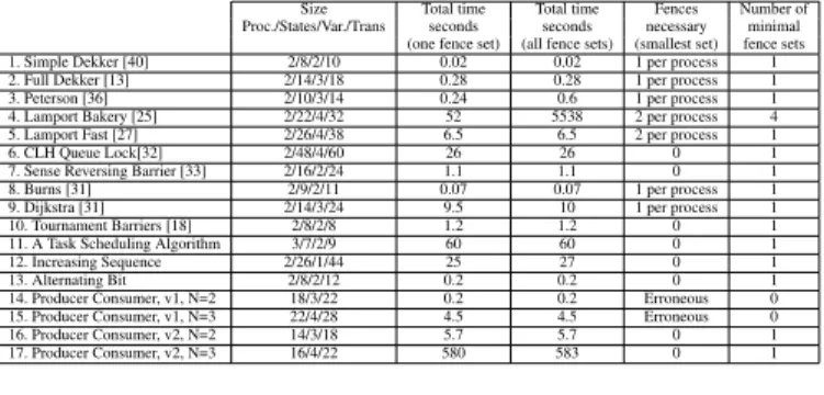
Outline In Section 2 we give an overview of our framework. In Section 3 we give some preliminaries. In Section 4 we introduce our model of concurrent programs, recall the formal model of TSO, and then introduce the SB semantics. In Section 5 we provide an al- gorithm for backward reachability analysis of programs under the SB semantics. We explain in Section 6 how we use the analysis to automatically derive all minimal sets of fences that ensure correct- ness of the program. In Section 7 we report on our experimental results. We make a detailed comparison with related work in Sec- tion 8. Finally, we give in Section 9 some conclusions and direc- tions for future research. The proofs of the lemmas, details of the implementation, and the experimental results are in the appendix.

2. Overview

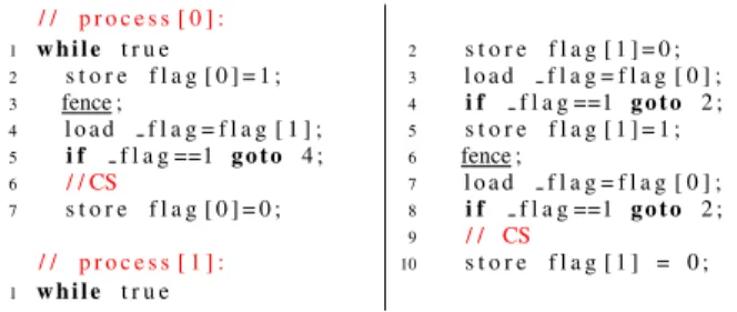
An Example Figure 1 shows the code for Burn’s mutual exclu- sion protocol, instantiated for two processes. It consists of a concur- rent program with two processes that repeatedly enter and exit their critical sections. We want the program to satisfy a safety property, namely that ofmutual exclusion. Checking such a safety property can be reduced to solving areachability problem: check whether the program will ever reach abad configuration, i.e., a configura- tion in which the two processes are both in their critical sections.

The program satisfies the specification under the SC semantics.

/ / p r o c e s s [ 0 ] :

1 w h i l e t r u e

2 s t o r e f l a g [ 0 ] = 1 ;

3 fence ;

4 l o a d f l a g = f l a g [ 1 ] ;

5 i f f l a g ==1 g o t o 4 ;

6 / / CS

7 s t o r e f l a g [ 0 ] = 0 ;

/ / p r o c e s s [ 1 ] :

1 w h i l e t r u e

2 s t o r e f l a g [ 1 ] = 0 ;

3 l o a d f l a g = f l a g [ 0 ] ;

4 i f f l a g ==1 g o t o 2 ;

5 s t o r e f l a g [ 1 ] = 1 ;

6 fence ;

7 l o a d f l a g = f l a g [ 0 ] ;

8 i f f l a g ==1 g o t o 2 ;

9 / / CS

10 s t o r e f l a g [ 1 ] = 0 ;

Figure 1. Burn’s Mutual Exclusion Algorithm. Local variables are prefixed with an underscore and the initial values of variables are 0.

Notice that the definitions of the two processes are not symmetric.

However, as we will see below, the program fails to satisfy its specification under TSO, if any of the fences is removed.

Total Store Order (TSO) A memory model is defined by the order in which the read (load) and write (store) operations are performed.

TheSequential Consistency (SC)semantics is the classical inter- leaving semantics, in which a trace of the system is an interleaving of traces of the different processes. In particular a store operation is visible to all processes immediately after it has been performed. In theTotal Store Order (TSO)semantics, read operations are allowed to overtake write operations of the same process if they concern different variables. More precisely, each process sees its own read and write operations exactly in the same order as it has issued them.

However, other processes may see older values than the one that has been stored by a process. TSO is thus also referred to as the store

→load order relaxation. Each possible execution of the program under the SC semantics is also possible under the TSO semantics.

However, the converse is not true. For example, if we remove the fences in Figure 1, the program does not satisfy mutual exclusion any more. In fact, as described below, there are at least two runs of the systems that can reach a bad configuration. Let us for the time being ignore the fences at lines 3 resp. 6 in the definitions of the processes.Run 1:process[1]reorders the read at line 7 with the write at line 5 as they concern different variables. As a result, process[1]can execute lines 1-4, then line 7, and before executing line 5,process[0]proceeds to the critical section asf lag[1]is still 0.

After that,process[1]can run lines 5 and 8 before also reaching the critical section and violating mutual exclusion.Run 2is obtained in a similar manner, now by lettingprocess[0]reorder lines 2 and 4.

Fence Insertion To eliminate the errors that may arise due to OoOEs (such as the ones described above for Burn’s protocol), pro- cessor vendors providefence operationsthat give the programmer more control over the executions of the program. More precisely, a fence inserted somewhere inside the program, restricts the reorder- ing of the operations before and after the fence: the operations be- fore the fence must take global effect before the execution of the operations after the fence. There are different types of fences de- pending on the operations they control (e.g., store-store or store- load). In the context of TSO, the relevant fence type is that of afull memory barrierthat prevents the reordering of all memory oper- ations. In the example of Figure 1, a fence is needed at line 6 in process[1]to forbidRun 1(the reordering of lines 5 and 7); and a fence is also needed at lines 3 inprocess[0]to preventRun 2. Ex- ecuting programs with fences is more costly than executing them without, and in fact inserting large numbers of fences goes against the spirit of OoOE as the program will approach its SC behavior.

Therefore, one reasonable criterion is to insert as few fences as pos- sible (provided that the set of inserted fences guarantees correctness of the program).

Reachability

Analysis Reachable?

No, the program is safe ProgramP

Specificationφ

Set of fencesF

No, the program can- not be made correct

Yes, add fences to the setF Conuter-Example

Analysis Fixable?

Placement ConstraintG

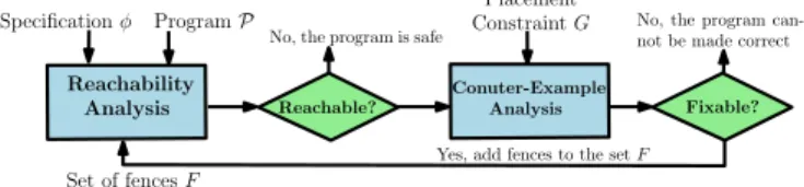
Figure 2. The flow of counter-example guided fence insertion.

Our Method Figure 2 gives an overview of our fence insertion procedure. Given a programPand a specification (a safety prop- ertyφ), the procedure finds the set of minimal sets of fences nec- essary in order to make thePcorrect wrt.φ. The procedure per- forms a counter-example guided refinement of sets of fences. More precisely, it maintains a set of candidate sets of fences that it will refine continuously during the run of the algorithm. The procedure starts optimistically by only having the empty set as a candidate (i.e., assuming that no fences are needed for correctness). Given a candidate setF, theReachability Analysismodule checks whether P^{, withF}inserted, satisfiesφ. This question is translated into the reachability of a set ofbad configurations. If no bad configuration

is reachable, we conclude thatF is sufficient for correctness and proceed to the next candidate set. Otherwise, the module returns a counter-example which will be provided to theCounter-Example Analysismodule. The module either generates new fences that need to be added toF or concludes that the program cannot be made correct, in which case the whole procedure terminates. The pro- cedure also terminates in case there are no other candidate sets to consider. The algorithm is parameterized by a predefinedplace- ment constraintwhich is a subsetGof all local states of the pro- cesses. The algorithm will place fences only after local states that belong toG. This gives the user the freedom to choose between the efficiency of the verification algorithm and the number of fences that are needed to ensure correctness of the program. The weakest placement constraint is defined by takingGto be the set of all local states of the processes, which means that a fence might be placed anywhere inside the program. On the other hand, one might want to place fences only after write operations, place them only before read operations, or avoid putting them within certain loops (e.g., loops that are known to be executed often during the runs of the program). For any givenG, the algorithm finds the minimal sets of fences that are sufficient for correctness. Below, we explain in more detail the main ingredients of the procedure.

Operational TSO Semantics Program verification requires a for- mal model of the system under verification. In our setting, this implies that we need a formal description of the TSO memory model. For this purpose, we use the operational semantics defined in [38, 40]. Conceptually, the model adds a FIFO buffer between each process and the main memory (cf. Figure 3). The buffer is used

p1

p2 Memory

x=2 y=7

y=1 y=3 x=5

y=8 y=5 y=10 y=6

Store x= 1 Loady

From the most recent write operation toyin the buffer

Loadx

Directly from the memory. There is no write operation toxin the buffer.

r0 r2

r1 r4

s0 s1

s2

Figure 3. Store buffers and the shared memory of a program under TSO. The size of the store buffer is unbounded.

to store the write operations performed by the process. Thus, a pro- cess executing a write instruction inserts it into its store buffer and immediately continues executing subsequent instructions. Memory updates are then performed by non-deterministically choosing a process and by executing the first write operation in its buffer (the left-most element in the buffer). A read operation by a processpon a variablexcan overtake some write operations stored in its own buffer if all these operations concern variables that are different fromx. Thus, if the buffer contains some write operations tox, then the read value must correspond to the value of the most recent such a write operation. Otherwise, the value is fetched from the memory.

A fence means that the buffer of the process must be flushed before the program can continue beyond the fence. The store buffers of the processes areunboundedsince there isa priorino limit on the number of write operations that can be issued by a process before a memory update occurs. For instance, in the program of Figure 1, the loop of lines 2–4 of process[1] may generate an unbounded num- ber of write operations (issued at line 2), and hence create an un- bounded number of elements inside the store buffer of process[1].

In fact, this still holds even after the insertion of fences since the inserted fences do not affect the operations inside the loop.

The SB Semantics The main obstacle in the design of the reach- ability algorithm is the fact the formal model of TSO [38] equips the processes with FIFO store buffers that are perfect and (poten- tially) unbounded. If one aims at ensuring correctness of the pro- gram regardless of the underlying (TSO) architecture, the sizes of the buffers cannot be pre-assumed. This gives rise to a difficult problem; it is well-known that the problem of checking safety prop- erties for finite-state processes communicating through unbounded FIFO channels is undecidable [7]. However, the TSO model does not exploit the full power of perfect FIFO buffers. This is demon- strated, for instance, by the fact that the reachability problem for finite-state programs running on TSO is in fact decidable [5]. Our goal is to exploit this in order to first design a method for algo- rithmic verification of programs running under the TSO semantics, and then use it to develop a method for automatic fence insertion.

Concretely, we will use the framework ofwell quasi-orderedtransi- tion systems [1, 16] in order to derive an algorithm for reachability analysis. The main challenge in using this framework is to define a pre-orderon the set of configurations, such that the transition relation ismonotonicwrt.(informally, monotonicity means that larger configurations can simulate smaller configurations). To de- rive such an ordering, we make the observation that a write opera- tion sent by one process to the buffer may never be noticed by the other processes. This is true since a value in the memory might be overwritten by other write operations before any other process has had time to read it. This suggests that we should define our order- ingto reflect the sub-word relation on the contents of the buffer.

(to be more concrete, the buffer of p₁ in Figure 3 can be viewed as the word[y=1][y=3][x=5]; and then[y=1][x=5]is one of its sub- words). The intuition would be that the extra write operations in the larger buffers of a process may after all never be noticed by the other processes, and hence a larger configuration should be able to simulate a smaller configuration. Unfortunately, as we will see in Section 4, the transition system induced by the TSO model is not monotonic wrt.. In order to circumvent this problem, we propose a new semantical model, namely the Single-Buffer (SB) semantics.

We defer the technical details of the SB semantics until Section 4, where we also explain how it is derived as an alternative to TSO.

Roughly speaking, a system in the SB semantics contains only one store buffer that is shared by all the processes (cf. Figure 5). On the other hand, each message inside the SB buffer contains a copy of the whole memory (rather than containing a write operation to a single variable, as in the case of TSO); together with a finite amount of “control data”. The SB model satisfies the two needed properties:

(i) it is equivalent to TSO (we can reduce he reachability problem under TSO to the one under SB); and (ii) its transition system is monotonic wrt. the sub-word relationon the (single) store buffer.

Reachability Analysis Given the pre-orderon the set of SB- configurations, we use the framework of [1, 16] to design our reach- ability analysis algorithm. Concretely, the algorithm works on in- finite sets of SB-configurations that are upward closed wrt. the or- dering. The algorithm performs backward reachability starting from the set of bad configurations (those violating the safety prop- erty). The monotonicity of the transition relation implies that all the generated sets are upward closed. Furthermore, termination of the algorithm is guaranteed sinceis awell quasi-ordering. In our instantiation of the algorithm, we use an automata-based formal- ism as a symbolic representation of upward closed sets of config- urations. If the safety property is violated, the algorithm returns a symbolic representation of a set of traces from which theCounter- Example Analysismodule can refine the set of fences.

Counter-Example Guided Fence Insertion A naive way to find the minimal fence sets is to simply try out all combinations. Obvi- ously, such an algorithm would not work in practice due to the large

number of possible combinations. Using the counter-examples pro- vided by our reachability algorithm, theCounter-Example Analysis module either finds new fences (satisfying the placement constraint G) to be added to the program, or it concludes that the program can- not be made correct (regardless of the number of inserted fences fromG). In the latter case, we can conclude that the program is incorrect even under the SC semantics (this holds provided thatG has been chosen so that it includes sources of all read operations or destinations of all write operations).

The fence refinement procedure means that the framework, as a whole, amounts to a counter-example guided fence insertion proce- dure, that automatically infers the minimal set of fences (satisfying a given fence placement constraint) that ensures the correctness of the program. The algorithm can be made to run until it has found all minimal sets of fences, or stop after finding the first set.

3. Preliminaries

In this section we first introduce notations that we use through the paper, and then define the notion of transition systems.

Notation We useNto denote the set of natural numbers. For sets AandB, we use[A7→B]to denote the set of all total functions from AtoBandf:A7→Bto denote thatfis a total function that mapsA toB. Fora∈Aandb∈B, we use f[a←-b]to denote the function f⁰defined as follows: f⁰(a) =band f⁰(a⁰) =f(a⁰)for alla⁰6=a.

LetΣbe a finite alphabet. We denote byΣ^∗(resp.Σ⁺) the set of allwords(resp. non-empty words) overΣ, and byεthe empty word.

The length of a wordw∈Σ^∗ is denoted by|w|; we assume that

|ε|=0. For everyi: 1≤i≤ |w|, letw(i)be the symbol at position iinw. Fora∈Σ, we writea∈wifaappears inw, i.e.,a=w(i)for somei: 1≤i≤ |w|. For wordsw1,w₂, we usew1·w2to denote the concatenation ofw₁andw₂. For a wordw6=εandi: 0≤i≤ |w|, we definewito be the suffix ofwthat we get by deleting the prefix of lengthi, i.e., the uniquew₂such thatw=w₁·w₂and|w₁|=i.

Transition Systems A transition system T ^{is a triple} (C,Init,−→) where C is a (potentially infinite) set of con- figurations, Init⊆C is the set of initial configurations, and

−

→ ⊆C×C is thetransition relation. We writec−→c⁰ to denote that(c,c⁰)∈ −→, and−→^∗ to denote the reflexive transitive closure of −→. A run π of T is of the form c0−→c1−→···−→cn, where ci−→ci+1 for all i: 0≤i< n. Then, we write c0 π

−→cn. We use target(π) to denote the configuration cn. Notice that, for configurations c,c⁰, we have that c−→^∗ c⁰ iff c−→^π c⁰ for some runπ. The runπis said to be acomputationifc0∈Init. Two runs π1 =c0−→c1−→···−→cm and π2 =cm+1−→cm+2−→···−→cn

are said to becompatibleifcm=cm+1. Then, we write π1•π2

to denote the run π1 = c0−→c1−→···−→cm−→cm+2−→···−→cn. Given an ordering v on C, we say that −→ is monotonic wrt.

v if wheneverc₁−→c⁰₁ and c₁vc₂, there exists ac⁰₂ such that c2−→∗ c⁰₂andc⁰₁vc⁰₂. We say that−→iseffectively monotonicwrt.

vif, given the configurationsc₁,c⁰₁,c₂ described above, we can computec⁰₂and a runπsuch thatc2 π

−→c⁰₂.

4. Concurrent Programs

We defineconcurrent programs, a model for representing shared- memory concurrent processes. A concurrent programPhas a fi- nite number of finite-state processes (threads), each with its own program code. Communication between processes is performed through a shared-memory that consists of a fixed number of shared variables (with finite domains) to which all threads can read and write. First, we define the syntax we use for concurrent programs.

Next, we introduce the TSO semantics including the transition sys- tems it induces and its reachability problem. Finally, we describe

informally the different features of the SB semantics, and the man- ner in which we derive them from the definition of TSO; and then we define formally its transition system and reachability problem.

4.1 Syntax

We assume a finite setX ofvariables ranging over a finite data domainV. Aconcurrent programis a pairP= (P,A)wherePis a finite set ofprocessesandA=

Ap|p∈P is a set of extended finite-state automata (one automatonApfor each process p∈P).

The automatonApis a triple Qp,q^init_p ,∆p

whereQpis a finite set oflocal states,q^init_p ∈Qpis theinitiallocal state, and∆pis a finite set oftransitions. Each transition is a triple(q,op,q⁰)whereq,q⁰∈ Qpandopis anoperation. An operation is of one of the following five forms: (1) the “no operation” nop, (2) the read operation r(x,v), (3) the write operation w(x,v), (4) the fence operation fence, and (5) theatomic read-write operationarw(x,v,v⁰), where x∈X, andv,v⁰∈V. For a transitiont= (q,op,q⁰), we usesource(t), operation(t), andtarget(t)to denoteq,op, andq⁰respectively. We defineQ:=∪p∈PQp and ∆:=∪p∈P∆p. A local state definition qis a mappingP7→Qsuch thatq(p)∈Qp for each p∈P. It is straightforward to translate programs in the form of Figure 1 to this model. Figure 4 is an automaton forprocess[0]in Figure 1.

L4,1 L5,1

L1,0 nop L2,0w(flag[0],1)L3,0fence L4,0 L5,0 L6,0 L7,0

nop

r(flag[1],1) r(flag[1],0)

r(flag[1],0) r(flag[1],1)

nop w(flag[0],0)

nop

Figure 4. The automaton of process[0]in Figure 1. Local states encode program locations and the value of the local variable flag.

4.2 TSO Semantics

We refer to Section 2 for an informal description TSO semantics.

Transition System We define the transition system induced by a program running under the TSO semantics. To do that, we define the set of configurations and transition relation. A TSO- configuration cis a triple q,b,mem

whereqis a local state defi- nition,b:P7→(X×V)^∗, andmem:X7→V. Intuitively,q(p)gives the local state of processp. The value ofb(p)is the content of the buffer belonging top. This buffer contains a sequence of write op- erations, where each write operation is defined by a pair, namely a variablexand a valuevthat is assigned tox. In our model, mes- sages will be appended to the buffer from the right, and fetched from the left. Finally,memdefines the state of the memory (defines the value of each variable in the memory). We useCTSOto denote the set of TSO-configurations. In Figure 3, we haveb(p1) = [y= 1][y=3][x=5],b(p2) = [y=8][y=5][y=10][y=6],mem(x) =2, andmem(y) =7 (to increase readability in the examples, we write the contents of the buffers in the form[y=1][y=3][x=5]in- stead of(y,1)(y,3)(x,5)). We define the transition relation−→TSO

onCTSO. The relation is induced by (1) members of∆; and (2) a set

∆⁰:=

update_p|p∈P whereupdate_p is an operation that up- dates the memory using the first message in the buffer of process p. For configurationsc= q,b,mem

,c⁰= q⁰,b⁰,mem⁰

, a process p∈P, andt∈∆p∪

update_p , we writec−→^t TSOc⁰to denote that one of the following conditions is satisfied:

•Nop:t= (q,nop,q⁰), q(p) =q, q⁰=q[p←-q⁰], b⁰=b, and mem⁰=mem. The process changes its state while the buffer contents and the memory remain unchanged.

•Write to store:t= (q,w(x,v),q⁰), q(p) =q,q⁰=q[p←-q⁰], b⁰=b[p←-b(p)·(x,v)], andmem⁰=mem. The write operation

is appended to the tail of the buffer. In Figure 3, executing a transition of the form(q,w(x,2),q⁰)∈∆p1would giveb⁰(p1) = [y=1][y=3][x=5][x=2].

•Update:t=update_p, q⁰=q,b=b⁰

p←-(x,v)·b⁰(p) , and mem⁰=mem[x←-v]. The write in the head of the buffer is removed and the memory is updated accordingly. In Figure 3, update_p1would giveb⁰(p1) = [y=3][x=5]andmem⁰(y) =1.

•Read: t = (q,r(x,v),q⁰), q(p) =q, q⁰=q[p←-q⁰], b⁰=b, mem⁰=mem, and one of the following conditions is satisfied:

Read own write: There is an i: 1≤i≤ |b(p)| such that b(p)(i) = (x,v), and(x,v⁰)6∈(b(p)i)for allv⁰∈V. If there is a write on xin the buffer of pthen we consider the most recent of such write operations (the right-most one in the buffer). This operation should assignvtox.

Read memory:(x,v⁰)6∈b(p)for allv⁰∈Vandmem(x) =v.

If there is no write operation onxin the buffer ofpthen the valuevofxis fetched from the memory.

In Figure 3,p₁can read the valuesx=5 andy=3, whilep₂ can read the valuex=2 andy=6.

•Fence:t= (q,fence,q⁰),q(p) =q,q⁰=q[p←-q⁰],b(p) =ε, b⁰=b, andmem⁰=mem. A fence operation may be performed by a process only if its buffer is empty.

•ARW:t= (q,arw(x,v,v⁰),q⁰),q(p) =q,q⁰=q[p←-q⁰],b(p) = ε,b⁰=b, mem(x) =v, andmem⁰=mem[x←-v⁰]. TheARW operation is performed atomically. It may be performed by a process only if its buffer is empty. The operation checks whether the value of variablexisv. In such a case, it changes its value tov⁰. Note this operation permits to model instructions like locked writes under x86-tso [22, 38] or compare-and-swap or swap under SPARC [40].

We use c−→^TSOc⁰ to denote thatc−→^{t TSO}c⁰for some t∈∆∪

∆⁰. The set InitTSO of initial TSO-configurations contains all configurations of the form qinit,binit,meminit

where, for allp∈P, we have thatqinit(p) =q^init_p andbinit(p) =ε. In other words, each process is in its initial local state and all the buffers are empty.

On the other hand, the memory may have any initial value. The transition system induced by a concurrent system under the TSO semantics is then given by(C_TSO,Init_TSO,−→TSO).

The TSO Reachability Problem Given a set Target of lo- cal state definitions, we use Reachable(TSO) (P) (Target) to be a predicate that indicates the reachability of the set q,b,mem

|q∈Target , i.e., whether a configurationc, where the local state definition ofcbelongs toTarget, is reachable. The reachability problem for TSO is to check, for a givenTarget, whetherReachable(TSO) (P) (Target)holds or not. Using stan- dard techniques we can reduce checking safety properties to the reachability problem. More precisely, we useTarget to denote

“bad configurations” that we do not want to occur during the ex- ecution of the system. For instance, in Burn’s protocol (Section 2), the bad configurations are those where the two processes are in line 6 resp. line 9 (corresponding to the critical sections of the two pro- cesses). Therefore, we often say that the “program is correct” to indicate thatTargetis not reachable.

4.3 Single-Buffer Semantics

As explained in Section 2, our goal is to derive a semantical model that is both equivalent to TSO and monotonic.

Informal Explanation Below, we motivate the different features of the SB semantics and explain how we derive them from the TSO semantics. To do that, we start from TSO and perform a number

of steps where we define new semantics SB1, SB2, SB3, until we arrive at the final definition of SB. The semantics introduced in each step is derived from the one in the previous step, by adding new features that are used to solve certain problems. These problems are illustrated through examples of concrete runs of the system.

First, we illustrate why the TSO semantics is not monotonic wrt.

the sub-word relation on the buffer contents. Recall that a system is monotonic if all the behaviors of a smaller configuration can also occur from a larger configuration. We consider a program with two processesp₁,p₂, where the automaton ofp₁contains the following two transitions:

q₀ q₁ q₂

p₁: r(x,1) r(y,0)

Consider a configurationc1where the local state of p1isq0, the memory containsx=0,y=0, the buffer of p1is empty, and the buffer ofp2 contains the word[x=1]. Then, according to the TSO semantics, there is a run of the system fromc1to a configuration where the local state ofp1isq2; the run simply updates the memory byx=1, and then performs the two read transitions. Consider the configurationc₂ where the buffer of p₂ now contains the word [y=1][x=1]. The local stateq₂is not reachable any more; we have to update the memory byx=1 (otherwise we cannot perform the read transition fromq0to stateq1). However, this implies that we have already updated the memory byy=1 which means that we cannot perform the read transition fromq1to stateq2. This violates monotonicity: some behavior of a smaller configurationc1is not a behavior of a larger configurationc2.

SB1.The problem with the above scenario is that we get a mem- ory configurationx=1,y=0 in the smaller configurationc1that is inconsistent with those we get fromc2. To cure this problem, we define SB1, where we let the processes send entire memory snap- shots to the buffer (rather than single write operations). In other words, each message in the buffer will now define the value of each variable in the program (rather than a single variable). The buffer contents of the configurationsc1 and c2 in step 1 will be of the forms[x=1,y=0]resp.[x=0,y=1] [x=1,y=1]. Notice that the buffer contents are not related by the sub-word relation, and hence the configurationsc₁,c₂do not violate monotonicity anymore. The problem with SB1 is that it is not equivalent to TSO; some behav- ior in SB1 is not possible in TSO. To see this, we consider two processesp1,p2whose automata contain the following transitions:

q₀ q₁

p₁: w(y,0)

r₀ r₁ r₂

p₂: w(x,1) r(x,0) Consider a configurationcwhere the local states ofp₁,p₂areq₀,r₀, the memory containsx=0,y=0, and the buffers are empty. There is no run fromcin TSO to a configuration where the local states areq1,r2sincep2 can only fetch the value 1 fromxonce the op- erationw(x,1)has been performed. However, such a configuration is reachable in SB1 as follows. The messages[x=1,y=0]byp2and [x=0,y=0]byp1are sent to the buffers and delivered to memory in that order. After these two operations, the memory value will be x=0,y=0, which allows the operationr(x,0)to be performed, hence the system reaches the statesq1,r2.

SB2.The problem in the above scenario is that the processes are not synchronized on memory updates, so a process may use some values that are not in the memory any more. In the above example, when p1 sends the memory snapshot forw(y,0) to its buffer, it should take the memory values contributed by other processes into consideration. Instead of sending [x=0,y=0]that contains an old value ofx, it should notice thatp2has changed the memory value ofxto 1 (by checking the most recent buffer message) and should hence send [x=1,y=0]. In SB2, we solve this problem by letting all the processes share a single buffer. Thus, the buffer contents

in the above run just before performing the last operationr(x,0) will be[x=1,y=0][x=1,y=0]and the read statement froms1tos2is not enabled any more. Again SB2 is not equivalent to TSO; some behavior of TSO is not possible under SB2. To see this, consider four processesp1,p2,p3,p4whose automata contain the following transitions:

q0 q1 q2

p1 :

w(x,1) w(x,2)

r0 r1 r2

p2 :

r(y,2) r(y,1)

s0 s1 s2

p3 :

w(y,1) r(x,1)

t0 t1 t2

p4 :

r(x,2) w(y,2)

Consider a configurationcwhere the local states of p1,p2,p3,p4

areq0,r0,s0,t0, the memory containsx=0,y=0, and the buffers are all empty. There is a run fromc in TSO to a configuration where the local states areq2,r2,s2,t2as follows: (i)p1sends[x=1]

followed by[x=2]to its buffer and moves toq2; (ii)p3sends[y=1]

to its buffer; (iii)[x=1]is updated to the memory from the buffer ofp1; (iv)p3readsx=1 from the memory and moves tos2; (v) [x=2]is updated to the memory from the buffer ofp1; (vi)p4reads x=2 from the memory and then sends[y=2]to its buffer moving to statet2; (vii)[y=2]is updated to the memory from the buffer ofp4; (viii)p2reads[y=2]from the memory; (ix)[y=1]is updated to the memory from the buffer ofp3; (x)p2readsy=1 from the memory and moves tor2. Such a run is not possible in SB2 according to the following reasoning. The write operationw(y,1)has to be sent to the buffer before the write operationw(y,2); otherwiser(x,2)is already performed and the value ofxin the memory will be equal (and remain) to 2 whenp₃ is in local states₁. Hence p₃ cannot perform the read transition froms₁ tos₂. In SB2, the operations in the buffer will be delivered to the memory in the same order as they entered the buffer. Sow(y,1)will be delivered to the memory before the write operationw(y,2). This means thatp2cannot fetch the valuey=2 from the memory before it fetches the valuey=1, and hencep2will not be able to reachr2.

SB3. The problem is that SB2 forces memory updates to be performed in the same order as the order of the corresponding write transitions even if these write transitions belong to different processes. For instance, in the above example, the write operation w(y,1)was performed before the write operation w(y,2). In the TSO semantics, the corresponding updates can be performed in the opposite order (since they belong to different buffers), while this is not allowed in SB2. In SB3, we remedy to this problem by providing the processes with a mechanism that allows them to update the memory independently of the other processes. More precisely, we add to each process a pointer to a position inside the buffer. From the point of view of the process, the buffer is divided by the pointer into three parts. The suffix of the buffer to the right of the pointer represents the sequence of write operations that have still not been used for memory updates. The position of the pointer itself represents the content of the memory, while the rest of the buffer (the prefix to the left of the pointer) is not relevant for the future behavior of the process (since it represents write operations that have already been used for updating the buffer). An update operation will then be simulated by moving the relevant pointer one step to the right. This adds the missing run mentioned above (cf.

Figure 5). First, the write operationsx=1 andx=2 are transferred to the buffer. Then, p4 moves its pointer to the position of the buffer wherex=2 sending the write operationy=2 to the buffer;

and thenp3moves its pointer to the position of the buffer where x=1 sending the write operationy=1 to the buffer. Now the write operationsy=1 andy=2 are in the correct order (y=2 before y=1). Therefore, p2can first move its pointer to the position in the buffer wherey=2 after which it moves its pointer one step to the right in the buffer wherey=1. In this manner, it is able to perform the two read transitions in the correct order.

q2 r2 s2 t2

x=0 y=0

p1

x=1 y=0 p1,x

p3

x=2 y=0 p1,x

p4

x=2

y=2 p4,y x=2 y=1 p3,y

p2

Figure 5. An SB-configuration.

SB.Finally, since the write operations of the different processes are now all mixed in the (single) buffer, we add also a mechanism that allows the processes to recognize the last write operations they have performed on each variable. Recall that in TSO, ifpreads the value ofxthen it will fetch the value from the most recent message in its buffer that represents a write operation onx(if such a message exists), instead of getting the value of x directly from the main memory (cf. Figure 3). To do this in SB, we equip each message in the buffer with a processpand a variablex, which denotes “p writes tox”. When a processpreadsx, it takes the value from the most recent message with(p,x)in the buffer (or from the memory if the buffer does not have such a message). As an example, the SB-configuration at the end of the above described computation is shown in Figure 5. Notice that an SB-configuration does not have an explicit representation of the main memory, as this is replaced by the pointers that represent the local views of the processes.

Finally, The orderingvon SB-configurations (formally defined in Section 5) is induced by the sub-word relation on the buffer contents. However, it will also reflect the last-write information on the variables, and the positions of the pointers inside the buffer.

Transition System Formally, an SB-configuration c is a triple q,b,z

whereqis (as in the case of the TSO semantics) a local state definition,b∈([X7→V]×P×X)⁺, andz:P7→N. Intuitively, the (only) buffer contains triples of the form(mem,p,x)wheremem defines the values of the variables (encoding a memory snapshot),x is the latest variable that has been written into, andpis the process that performed the write operation. Furthermore,zrepresents a set ofpointers(one for each process) where, from the point of view of p, the wordbz(p) is the sequence of write operations that have not yet been used for memory updates and the first element of the tripleb(z(p)) represents the memory content. We useCSB

to denote the set of SB-configurations. As an example, in the SB- configuration of Figure 5, the pointer ofp4points to the message [x=2,y=0,(p1,x)]. This means that the current view of p4 is that the memory contains x=2 andy=0. From the point of view ofp₄, the word[x=2,y=2,(p₄,y)][x=2,y=1,(p₃,y)]represents those write operations that have not yet been delivered to the memory. As we shall see below, the buffer will never be empty, since it is not empty in an initial configuration, and since no messages are ever removed from it during a run of the system (in SB semantics, the update operation moves a pointer to the right instead of removing a message in the buffer). This implies (among other things) that the invariantz(p)>0 is always maintained.

Letc= q,b,z

be an SB-configuration. For everyp∈Pand x∈X, we useLastWrite(c,p,x)to denote the index of the most recent buffer message wherepwrites toxor the message with the current memory ofpif the aforementioned type of message does not exist in the buffer. For example, letcbe the configuration in Figure 5, thenLastWrite(c,p1,x) =3,LastWrite(c,p1,y) =1, LastWrite(c,p4,y) =4, andLastWrite(c,p3,x) =2. Formally, LastWrite(c,p,x) is the largest index i such that i=z(p) or b(i) = (mem,p,x)for somemem.

We define the transition relation −→SB on the set of SB- configurations as follows. In a similar manner to the case of TSO, the relation is induced by members of∆∪∆⁰. For configurations c= q,b,z

, c⁰= q⁰,b⁰,z⁰

, andt∈∆p∪

update_p , we write c−→^t SBc⁰to denote that one of the following conditions is satisfied:

•Nop:t= (q,nop,q⁰), q(p) =q, q⁰=q[p←-q⁰], b⁰=b and z⁰=z. The operation changes only local states.

•Write to store:t=(q,w(x,v),q⁰),q(p)=q, q⁰=q[p←-q⁰], b(|b|) is of the form(mem1,p1,x1),b⁰=b·(mem1[x←-v],p,x), and z⁰=z. A new message is appended to the tail of the buffer. The values of the variables in the new message are identical to those in the previous last message except that the value ofxhas been updated tov. Moreover, we include the updating processpand the updated variablex. Below is an example ofp1writes tox.

q2 r2

x=0 p1,p2

(q₀,w(x,1),q₁)

−−−−−−−−−→SB

q2 r2

x=0 p1,p2

x=1 p1,x

•Update: t=update_p, q⁰=q, b⁰= b, z(p)<|b| and z⁰ = z[p←-z(p) +1]. An update operation performed by a process pis simulated by moving the pointer ofpone step to the right.

This means that we remove the oldest write operation that is yet to be used for a memory update. The removed element will now represent the memory contents from the point of view ofp. For example,update_p4 moves the pointer ofp4 in Figure 5 from [x=2,y=0,(p1,x)]to[x=2,y=2,(p4,y)].

•Read:t= (q,r(x,v),q⁰),q(p) =q,q⁰=q[p←-q⁰],b⁰=b, and b(LastWrite(c,p,x)) = (mem1,p1,x1)for somemem1,p1,x1

with mem1(x) =v. As an example, suppose that p1 reads the variablexin the configuration of Figure 5. The message b(LastWrite(c,p1,x)) = [x=2,y=0,(p1,x)]. It follows that a transition with read operationr(x,v)is enabled only whenv=2.

•Fence:t= (q,fence,q⁰),q(p) =q,q⁰=q[p←-q⁰],z(p) =|b|, b⁰=b, andz⁰=z. The buffer should be empty from the point of view ofpwhen the transition is performed. This is encoded by the equalityz(p) =|b|. In Figure 5,p2is the only process that can execute a fence operation (its buffer is empty).

•ARW:t= (q,arw(x,v,v⁰),q⁰),q(p) =q,q⁰=q[p←-q⁰],z(p) =

|b|, b(|b|) is of the form(mem₁,p₁,x₁), mem₁(x) =v, b⁰= b·(mem1[x←-v⁰],p,x), andz⁰=z[p←-z(p) +1]. The fact that the buffer is empty from the point of view of pis encoded by the equalityz(p) =|b|. The content of the memory can then be fetched from the right-most elementb(|b|)in the buffer. To encode that the buffer is still empty after the operation (from the point of view ofp) the pointer ofpis moved one step to the right. In Figure 5,p2is the only process that can execute this type of transition.

We use c−→SBc⁰ to denote that c−→^t SBc⁰ for some t∈∆∪∆⁰.

q0 r0 s0 t0

x=0 y=0

p1,p2,p3,p4

The set Init_SB of initialSB-configurations (the figure on the right is an example of an initial SB-configuration) contains all configurations of the form q_init,b_init,z_init

where|b_init|=1, and

for allp∈P, we have thatq_init(p) =q^init_p , andz_init(p) =1. In other words, each process is in its initial local state. The buffer contains a single message, say of the form(meminit,pinit,xinit), wherememinit

represents the initial value of the memory. The memory may have any initial value. Also, the values ofpinitandxinitare not relevant since they will not be used in the computations of the system. The pointers of all the processes point to the first position in the buffer.

According to our encoding, this indicates that their buffers are all empty. The transition system induced by a concurrent system under the SB semantics is then given by(C_SB,Init_SB,−→SB).

The SB Reachability Problem We define the predicate Reachable(SB) (P) (Target), and define the reachability problem for the SB semantics, in a similar manner to the case of TSO. The following theorem states equivalence of the reachability problems under the TSO and SB semantics. Due to the technicality of the proof and to the lack of space, we leave it for the appendix.

THEOREM4.1. For a concurrent program P and a local state definitionTarget, the reachability problems are equivalent under the TSO and SB semantics.

5. The SB Reachability Algorithm

In this section, we present an algorithm for checking reachabil- ity of an (infinite) set of configurations characterized by a (finite) setTargetof local state definitions. In addition to answering the reachability question, the algorithm also provides an “error trace”

in caseTargetis reachable. First, we define an orderingvon the set of SB-configurations, and show that it satisfies two important properties, namely (i) it is a well quasi-ordering (wqo), i.e., for every infinite sequencec0,c₁, . . . of SB-configurations, there are i< jwithcivcj; and (ii) that the SB-transition relation−→SBis monotonic wrt.v. The algorithm performs backward reachability analysis from the set of target configurations. During each step of the search procedure, the algorithm takes the upward closure (wrt.

v) of the generated set of configurations. By monotonicity ofvit follows that taking the upward closure preserves exactness of the analysis. From the fact that we always work with upward closed sets and thatvis a wqo it follows that the algorithm is guaran- teed to terminate. In the algorithm, we use a variant of finite-state automata, calledSB-automata, as a symbolic representation of (po- tentially infinite) sets of SB-configurations. Assume a concurrent programP= (P,A).

Ordering For an SB-configuration c = q,b,z

we define ActiveIndex(c):=min{z(p)|p∈P}. In other words, the part of bto the right of (and including)ActiveIndex(c)is “active”, while the part to the left is “dead” in the sense that all its content has al- ready been used for memory updates. The left part is therefore not relevant for computations starting fromc. For example, in Figure 5, the active index is 1, i.e., all of its buffer messages are still alive.

Letc= q,b,z

andc⁰= q⁰,b⁰,z⁰

be two SB-configurations.

Define j:=ActiveIndex(c) and j⁰:=ActiveIndex(c⁰). We writecvc⁰to denote that (i)q=q⁰and that (ii) there is an injection g:{j,j+1, . . . ,|b|} 7→ {j⁰,j⁰+1, . . . ,|b⁰|}such that the following conditions are satisfied. For everyi,i1,i2∈ {j, . . . ,|b|}, (1)i1<i2

impliesg(i1)<g(i2), (2)b(i) =b⁰(g(i)), (3)LastWrite(c⁰,p,x) = g(LastWrite(c,p,x)) for all p∈P andx∈X, and (4)z⁰(p) = g(z(p))for all p∈P. The first condition means thatgis strictly monotonic. The second condition corresponds to the fact that the activepart ofbis asub-wordof theactivepart of b⁰. The third condition ensures that the last write indices wrt. all processes and variables are consistent. The last condition ensures that each pro- cess points to identical elements inbandb⁰. Below is an example of two configurationscandc⁰such thatcvc⁰.

c^{0 q}r2²

x=0 x=5 p1,x x=6 p2,x p1,p2

x=3 p1,x x=9 p1,x

c ^qr2²

x=0 x=6 p2,x

p1,p2

x=9 p1,x

We get the following lemma from the fact that (i) the sub- word relation is a well-quasi ordering on finite words [19], and that (ii) the number of states and messages (associated with last write operations and pointers) that should be equal, is finite.

LEMMA5.1.The relation v is a well-quasi ordering on SB- configurations.

The following lemma shows effective monotonicity of the SB- transition relation wrt. v. As we shall see below, this allows the reachability algorithm to only work with upward closed sets.

Monotonicity (among other things) implies the termination of the reachability algorithm. The effectiveness aspect will be used in the fence insertion algorithm (cf. Section 6).

LEMMA5.2. −→^SBis effectively monotonic wrt.v.

Recall that the termeffective monotonicityis defined in Section 3.

Theupward closureof a setCof SB-configurations is defined as C↑:={c⁰|∃c∈C,cvc⁰}. The setCisupward closedifC=C↑. SB-Automata First we introduce an alphabet Σ :=

([X7→V]×P×X)×2^P. Each element ((mem,p,x),P⁰) ∈ Σ represents a single position in the buffer of an SB-configuration.

More precisely, the triple (mem,p,x) represents the message stored at that position and the set P⁰ ⊆P gives the (possibly empty) set of processes whose pointers point to the given position.

Consider a wordw=a1a2···an ∈Σ^∗, where ai is of the form ((memi,pi,xi),Pi). We say thatw is proper if, for each process p∈P, there is exactly onei: 1≤i≤nwithp∈Pi. In other words, the pointer of each process is uniquely mapped to one position inw. A proper wordwof the above form can be “decoded” into a (unique) pairdecoding(w):= (b,z), defined by (i)|b|=n, (ii) b(i) = (memi,pi,xi)for alli: 1≤i≤n, and (iii)z(p)is the unique integeri: 1≤i≤nsuch thatp∈Pi(the value ofiis well-defined sincewis proper). We extend the function to sets of words where decoding(W):={decoding(w)|w∈W}. Below is a proper word corresponding to the buffer and pointers in Figure 5.

[x=0,y=0,∗],{p1} [x=1,y=0,p1,x],{p3} [x=2,y=0,p1,x],{p4} [x=2,y=2,p4,y],0/ [x=2,y=1,p3,y],{p2}

An SB-automatonAis a tuple S,∆,S^final,h

whereSis a finite set ofstates,∆⊆S×Σ×Sis a finite set of transitions,S^final⊆S is the set offinalstates, andh:(P7→Q)7→S. The total function hdefines a labeling of the states ofAby the local state definitions of the concurrent programP, such that eachqis mapped to a state h(q)inA. Examples of SB-automata can be found in Figure 6. For a states∈S, we defineL(A,s)to be the set of words of the formw= a1a2···ansuch that there are statess0,s1, . . . ,sn∈Ssatisfying the following conditions: (i)s0=s, (ii)(si,ai+1,si+1)∈∆for alli: 0≤ i<n, (iii)sn∈S^final, and (iv)wis proper. We define thelanguage ofAbyL(A):=

q,b,z

|(b,z)∈decoding L A,h(q) . Thus, the languageL(A)characterizes a set of SB-configurations. More precisely, the configuration q,b,z

belongs to L(A) if (b,z) is the decoding of a word that is accepted byAwhen Ais started from the stateh(q) (the state that is labeled by q). A setC of SB-configurations is said to beregularifC=L(A)for some SB- automatonA.

Operations on SB-Automata We show that we can compute the operations needed for the reachability algorithm. First, observe that regular sets of SB-configurations are closed under union and intersection. For SB-automataA1,A2, we useA1∩A2to denote an automatonAsuch thatL(A) =L(A1)∩L(A2). We defineA1∪A2

in a similar manner. We useA^0/to denote an (arbitrary) automaton whose language is empty. We can construct SB-automata for the set of initial SB-configurations, and for sets of SB-configurations characterized by local state definitions.

LEMMA5.3. We can compute an SB-automaton A^init such that L A^init

= InitSB. For a set Target of local state defini- tions, we can compute an SB-automaton A(Target) such that L(A(Target)):=

q,b,z

|q∈Target .

The following lemma tells us that regularity of a set is preserved by taking upward closure, and that we in fact can compute the automaton that describes the upward closure.

LEMMA5.4. For an SB-automaton A we can compute an SB- automaton A↑such that L(A↑) =L(A)↑.

We define the predecessor functionas follows. Lett∈∆∪∆⁰ and letC be a set of SB-configurations. We define Pret(C):=

{c|∃c⁰∈C,c−→^t SBc⁰}to denote the set of immediate predecessor