The Spatial Development of India

Policy Research Working Paper 6060

The Spatial Development of India

Klaus Desmet Ejaz Ghani Stephen D. O’Connell Esteban Rossi-Hansberg

The World Bank South Asia Region

Poverty Reduction and Economic Management Unit May 2012

WPS6060

Public Disclosure Authorized Public Disclosure Authorized Public Disclosure Authorized Public Disclosure Authorized

Produced by the Research Support Team

Abstract

The Policy Research Working Paper Series disseminates the findings of work in progress to encourage the exchange of ideas about development issues. An objective of the series is to get the findings out quickly, even if the presentations are less than fully polished. The papers carry the names of the authors and should be cited accordingly. The findings, interpretations, and conclusions expressed in this paper are entirely those of the authors. They do not necessarily represent the views of the International Bank for Reconstruction and Development/World Bank and its affiliated organizations, or those of the Executive Directors of the World Bank or the governments they represent.

Policy Research Working Paper 6060

In the last two decades the Indian economy has been growing unabatedly, with memories of the Hindu rate of growth rapidly fading. But this unprecedented growth has also resulted in widening spatial disparities. While cities such as Hyderabad have emerged as major clusters of high development, many rural areas have been left behind with little development benefits accruing to them.

India’s mega-cities have continued to grow. This situation raises a number of important policy questions. Should

This paper is a product of the Poverty Reduction and Economic Management Unit, South Asia Region. It is part of a larger effort by the World Bank to provide open access to its research and make a contribution to development policy discussions around the world. Policy Research Working Papers are also posted on the Web at http://econ.worldbank.org. The authors may be contacted at Eghani@worldbank.org, soconnell@gc.cuny.edu, klaus.desmet@gmail.com, and erossi@princeton.edu.

India aim to spread development more equally across

space? Are India’s cities becoming too large? Should the

government invest in infrastructure in the large cities

to reduce congestion or in medium-sized locations to

facilitate the emergence of new economic clusters? What

are the tradeoffs between agglomeration economies and

congestion costs? How different is Indias experience

compared with China and USA?

The Spatial Development of India

Klaus Desmet (Universidad Carlos III), Ejaz Ghani (World Bank), Stephen D. O’Connell (World Bank),

and Esteban Rossi-Hansberg (Princeton University)

JEL No. J61,L10,L60,O10,O14,O17,R11,R12,R13,R14,R23

2 1. Introduction

In the last two decades, the Indian economy has been growing unabatedly, with memories of the Hindu rate of growth rapidly fading. But that development has led to widening spatial disparities. While cities such as Hyderabad have emerged as major clusters of high development, certain rural areas have been left behind. India's mega-cities have continued to grow, fed by a steady stream of migrants from the countryside. This situation raises a number of important policy questions. Should India aim to spread development more equally across space? Are India’s cities becoming too large? Should the government invest in infrastructure in the large cities to reduce congestion or in medium-sized locations to facilitate the emergence of new economic clusters?

Though such spatial inequalities are not unfamiliar from other countries, there is a relevant difference: India’s growth has mainly stemmed from a rapidly expanding service sector. This is important in the light of recent work by Desmet and Rossi-Hansberg (2009) who have shown that manufacturing and services exhibit very different spatial growth patterns in the U.S. and Europe. In the last decades U.S. and European manufacturing has been dispersing from high-density clusters to less dense areas, whereas services have been experiencing increasing concentration, except for the densest locations where congestion is the dominating force. Desmet and Rossi-Hansberg (2009) relate these opposing patterns to the differential impact of ICT (Information and Communication Technology) on both sectors. They argue that the diffusion of general purpose technologies, such as ICT, leads to knowledge spillovers that are enhanced by spatial concentration and the emergence of high-density clusters of economic activity. In recent decades we have seen this phenomenon unfold in services, as ICT is disproportionately benefitting that sector, but that paper shows that something similar occurred in manufacturing, which was profoundly and unevenly affected by electrification, at the beginning of the 20

century.

A first question, then, is whether India exhibits the same distinction between manufacturing and services. Although services are clearly benefitting from ICT, so that we would expect to observe a tendency towards spatial concentration in India, it is less clear how manufacturing should behave in that country. Although manufacturing is now dispersing in the U.S., this tendency only started in the post-World War II period. Given that manufacturing in India is not as mature a sector as in the U.S., the tendency towards dispersion might very well be weaker.

A second question is whether the tradeoff between agglomeration economies and congestion costs in

India is similar to the one in the U.S. or Europe. Casual observation suggests that the costs of

congestion in India’s mega-cities are huge, implying that there should be decreasing returns to further

expansion. However, these mega-cities may also benefit from relatively large agglomeration

3

economies, compared to medium-sized cities that might suffer from market access problems, lack of intermediate goods and infrastructure, and other impediments to grow fast. In the developed world this problem may be less severe, thus providing growth opportunities to medium-sized locations that are not present in India. Comparing the U.S. and India in the service sector, we indeed find that agglomeration economies peak for intermediate-sized locations in the U.S., whereas the large mega- cities are the winners in India. This finding is not common to all emerging economies. Although for want of high quality sectoral employment data at the local level we refrain from an in-depth study of China, our preliminary exploration suggests that China looks more similar to the U.S. in that decreasing returns dominate in high-density cities. The finding that “India is different”, because of both the failure of medium-density locations to grow faster and the importance of its service sector, justifies studying the spatial development of that country in further detail.

2. Data

To study employment dynamics across space in India, a first issue is to decide on the level of spatial disaggregation at which we have reliable data. India is divided into 35 states (or union territories) and 640 districts. While certainly the quality of the data are more reliable at the state than at the district level, work on the U.S. by Desmet and Rossi-Hansberg (2009) shows that having a high degree of spatial disaggregation is important. Indeed, agglomeration economies and congestion effects may get lost at higher levels of aggregation, so that focusing on districts is better. In addition, having a broad distribution of places (going from small to intermediate to large) is also important, since previous work for the U.S. has shown that the scale-dependence of growth may be non-linear.

India does not collect comprehensive sectoral employment data at the district level. We therefore rely

on micro-data from surveys. India runs two firm-level surveys, the Annual Survey of Industries (ASI)

and the one conducted by the National Sample Survey Organisation (NSSO). The ASI survey has

information on the so-called organized manufacturing sector (essentially comprising of firms with

more than 10 workers), whereas the NSSO covers the unorganized manufacturing sector and the

services sector. Both surveys, the ASI and the NSSO, overlap for the fiscal years 1989-90, 1994-95,

2000-01 and 2005-06. However, the service sector has only been surveyed more recently, in fiscal

years 2001-02 and 2006-07. Given that part of our focus will be on the difference between

manufacturing and services, we will use 2000-2005 for manufacturing and 2001-2006 for services.

4

For the case of manufacturing, the ASI covers all registered factories, and uses a sampling frame that is stratified at the state and the four-digit National Industry Classification (NIC) level. We complement these data by the NSSO which covers all unorganized manufacturing enterprises. In the case of the NSSO the sample stratification is more sophisticated and includes both the district level and the two-digit NIC sectors. For the case of services, the NSSO follows a similar stratification, including the district and the two-digit NIC sectors. Note, however, that some service subsectors, such as retail, wholesale and financial services, are excluded in at least one of the two available years.

Furthermore, as the NIC definitions have changed over time, we make them consistent using concordances that come with the data.

Sampling weights provided by the separate survey datasets are then applied to create population-level estimates of total employment by district and sector. One obvious issue regards the reliability of this procedure and possible measurement error. To address this issue, we do a number of robustness checks. In particular, we complement our estimation of district-level sectoral employment from firm surveys by an alternative measure using the Employment-Unemployment Survey, frequently referred to as the Labor Force Survey, carried out by the NSSO in fiscal years 1999-2000 and 2004-05. This survey collects individual-level information on location, occupational status and industry of occupation detailed enough to allow an estimation of employment by NIC industry and district. The sample stratification is similar to that of the NSSO. We run robustness checks using both major sources of data, the one based on firm-level surveys and the other based on individual-level surveys.

A last concern is that sometimes districts have been redefined, combined, or split. For these types of changes we follow a simple strategy for assuring consistent district definitions over time. In the case of a single district being divided into two or more “new” districts, we recreate the original district by combining the new districts (backward-compatibility). When two or more previous districts are combined, we recreate the new combined districts in the earlier years (forward-compatibility). In the case of transfers of land between districts we combine the districts involved in all periods.

3. The Spatial Evolution of India

1

When compairing the results with the U.S., we will make the definition of services in both countries comparable.

2

Nataraj (2009), Kathuria et al. (2010), Hasan and Jandoc (2010) and Dehejia and Panagariya (2010) provide

detailed overviews of similarly constructed databases. See also Fernandes and Pakes (2010) for a description of

the Indian manufacturing sector.

5

This section analyzes the spatial evolution of employment in India. Although most research on India has focused on the manufacturing sector, we will distinguish between manufacturing and services for two reasons. First, given the emergence of India as a service-based economy, it is key to understand which types of locations are benefiting from the country’s structural transformation (Ghani, 2010).

Second, as already pointed out, the work by Desmet and Rossi-Hansberg (2009) has documented important differences between the spatial dynamics of manufacturing and services in the U.S. We want to see whether the same patterns show up in India.

Given the possible importance of nonlinearities in the scale-dependence of growth, we run nonlinear kernel regressions of the form:

where

is log of sectoral employment density in year t, district i and sector j. The estimation uses an Epanechnikov kernel with bandwidth 0.8.

Because the distribution of employment density levels is approximately log-normal, we focus on the log of employment density. To facilitate interpretation, we will plot annual employment growth as a function of initial log employment density in the same industry. In this case, a negative slope indicates de-concentration (convergence) and a positive slope indicates concentration (divergence).

Before we present our findings it is important to discuss the implications that one can draw from looking at this evidence. Desmet and Rossi-Hansberg (2009) provide a theory of the spatial evolution of economic activity in which the relationship between local employment growth in an industry and the density of employment in that location is the result of three main forces. First, high land prices in dense locations will create incentives for firms in an industry to move to locations where land rents are lower. Second, congestion costs in large locations, due to high transport costs, pollution, and local fixed factors also contribute to the dispersion of employment in an industry. Third, industry spillovers, pecuniary externalities, labor market pooling, etc., all facilitated by high density, constitute an agglomeration force that leads to further concentration of employment. Looking at the relationship between employment growth and employment density can then reveal which of these forces dominates for particular levels of density. For example, a declining relationship between employment growth rates and employment densities would imply that the two dispersion forces dominate the agglomeration forces. In contrast, if the observed relationship is positive, it implies that agglomeration forces dominate congestion ones. In general, this relationship varies between locations

3

We also experimented with using an optimal bandwidth. This does not change the qualitative results, but

makes the comparison between graphs more difficult. Further details of this methodology can be found in

Desmet and Fafchamps (2006).

6

with different employment density and over time, and it represents the evolution of a spatial economy. Furthermore, the presence of agglomeration forces that have not yet been balanced by congestion forces indicates the benefits of concentrating production in locations with higher employment density. Throughout the rest of this paper, we use the lens provided by this empirical relationship, interpreted using the theory in Desmet and Rossi-Hansberg (2009), to shed light on the spatial development of India.

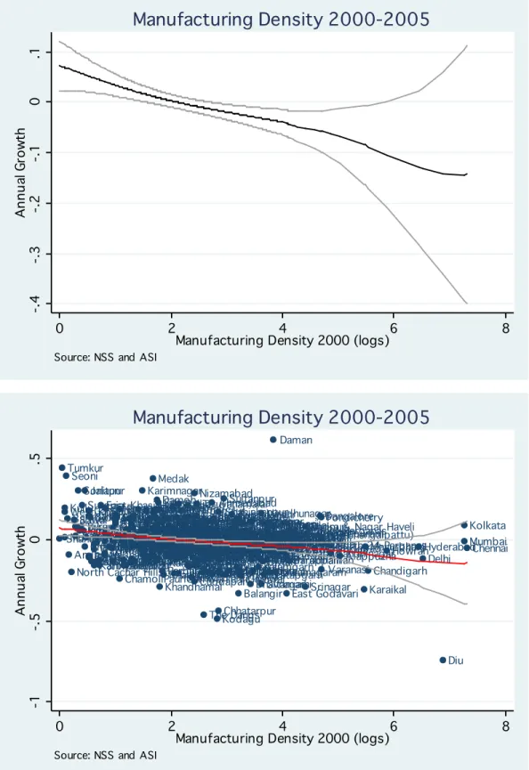
Figure 1 shows annual manufacturing employment growth as a function of initial manufacturing employment density (in logs). In this benchmark exercises the employment data at the district level have been constructed from firm-level surveys (NSS and ASI). The picture suggests that manufacturing is dispersing through space. Low-density manufacturing districts are growing faster than high-density manufacturing districts. Note, however, that the 95% confidence intervals are extremely large in the upper tail, suggesting a rather weak relation between scale and growth for high- density locations. Indeed, as can be seen from the bottom panel of Figure 1, some of the large cities, such as Kolkata and Mumbai, are experiencing higher growth than that predicted by the kernel regression.

Services show a distinctly different pattern. As can be seen from Figure 2, although low and medium- density service locations exhibit spatial dispersion, for the high-density service locations we observe increasing concentration. That is, the high-density service clusters are gaining relative to those locations with slightly lower employment density. In contrast to findings for the U.S. and Europe, high-density service clusters do not seem to be running into decreasing returns. The bottom panel of Figure 2 shows that many of the well-known IT clusters are in the upward-sloping part of the estimated relation, suggesting that they are benefitting from agglomeration economies. For example, service employment in Hyderabad and Chennai are growing at an annual rate of, respectively, 11%

and 4%. If we were to run a simple regression, the predicted growth rate of these two cities would be, respectively, -7.1% and -8.2%. This underscores the importance of taking into account non-linearities in the scale-dependence of growth. Note that the upward-sloping part is also driven by some of the country’s largest cities, such as Mumbai. However, not all large cities exhibit high growth in services.

As a robustness check, we re-run these same kernel regressions, using sectoral employment at the

district level constructed from the LFS. The results are shown in Figures 3 and 4. In the case of

services, we confirm our previous findings: there is clear evidence of increasing concentration in the

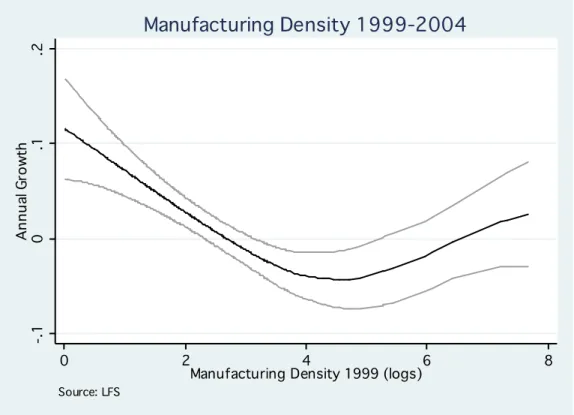
upper tail. However, for manufacturing the results look quite different. While in Figure 1 we

observed spatial dispersion throughout the distribution (though insignificant in the upper-tail), we

now find, as in services, evidence of spatial concentration for high-density manufacturing clusters.

7

This is consistent with our observation that some of the large cities continue to experience relatively strong manufacturing employment growth. According to the LFS, Kolkata, for example, is growing at an annual rate of 4.8%.

In addition to this robustness analysis, we run a number of further checks by, for example, taking the average of district employment coming from the NSS and the LFS, or by dropping all observations for which the difference in growth rates in the NSS and the LFS is above a certain threshold. These further robustness checks confirm that there is strong evidence of agglomeration economies for high-density service clusters, with weaker evidence of the same phenomenon in the manufacturing sector.

The existence of agglomeration economies in services is consistent with findings for the U.S. and Europe. The weak evidence for such agglomeration economies in manufacturing contrasts with the tendency towards dispersion across the entire distribution in the case of the U.S. and Europe. One possible reason for this difference between India and Europe may be related to the theory of Desmet and Rossi-Hansberg (2009). They argue that different spatial growth patterns arise in different industries, depending on the industry’s “age”, defined as the time elapsed since it was last affected by a general purpose technology (GPT). By that token, in the U.S. services is a “young” industry (as it is still experiencing the impact of ICT), whereas manufacturing is a “mature” industry (as the last major GPT in that sector, electrification, goes back to the early 20

century). But of course the age of an industry in one country need not be the same as its age in another country. It could be argued that not only the service industry in India is younger than the manufacturing industry in India, but also that the manufacturing industry in India is younger than the manufacturing industry in the U.S. If so, finding some remnants of (weak) agglomeration economies in the manufacturing sector in India is not surprising. In this respect it is relevant to note that the manufacturing industry in the U.S.

continued to exhibit evidence of agglomeration economies for intermediate-sized locations until the 1940s.

Although our main distinction is between the manufacturing and the service sector, obviously there are important differences between different subsectors within manufacturing and within services.

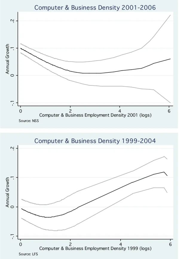
Using the definition of “age” of Desmet and Rossi-Hansberg (2009), business & computers services

are a particularly young subsector. There is ample evidence that business & computer services have

benefitted disproportionately from ICT (Chun et al., 2005; Caselli and Paternò 2001; McGuckin and

8

Stiroh, 2002). Figure 5 shows the kernel regression, based on both the NSS (upper panel) and LFS (lower panel). We observe a clear tendency towards increasing spatial concentration.

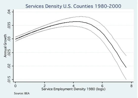
Although the service sector in India shows some similarities with the service sector in the U.S.  both exhibit agglomeration economies  there is one important difference: as can be seen from comparing Figure 2 and Figure 6, in the U.S. agglomeration economies in services dominate for medium-density locations, whereas in India agglomeration economies dominate for high-density locations.

In principle, there could be two possible explanations for this finding. Either the high- density service clusters in India have a lower density than the high-density service clusters in the U.S., or the tradeoff between agglomeration economies and congestion costs is different in both countries.

Given that we have used the same scaling to draw Figure 2 and Figure 6 it is clear that for similar high-density service clusters, congestion dominates in the U.S. whereas agglomeration economies dominate in India. According to our findings, agglomeration economies in the U.S. service sector peak at a density of between 50 and 150 employees per square kilometer. Three of the main high- tech counties in the U.S. fall within that range: Santa Clara, Calif. (Silicon Valley), Middlesex, Mass.

(Route 128) and Durham, NC (Research Triangle). In contrast, in India, agglomeration economies increase in the upper tail of the distribution, in places, such as Hyderabad and Chennai, with service employment densities reaching into the thousands. For those levels of density, U.S. locations exhibit substantial congestion.

In as far as the allocation of activity across space is efficient in the U.S., this suggests that there are forces restricting growth in medium-density places in India, making the high-density locations relatively more attractive. In other words, it might be the case that the high-density clusters in India are more successful, not because of the lack of congestion in the mega-cities but because of the absence of agglomeration economies in medium-sized locations. Certain policies or frictions, such as a lack of general infrastructure, may prevent these medium-sized cities from growing faster.

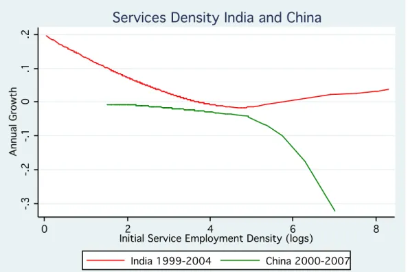
In that sense it may be suggestive to compare India’s experience not just to the U.S., but also to another large emerging economy, China. Figure 7 compares India and the U.S., whereas Figure 8 compares India and China. Before discussing the results, a word of caution about the data we use for

4

To make all the figures comparable, the scale of the horizontal axis is always the same (i.e. observations below 0 are not shown). If we were to show smaller places, we would find evidence of convergence in low-density districts.

5

Our regressions for the U.S. take counties as the unit of observation. To make the definition of services as

similar as possible to the one in the U.S. we are using the sum of transport & utilities and other services from

the BEA. Using broader definitions of services by including, say, retail and wholesale, do not change the

findings.

9

China: the employment figures measure the number of “staff and workers”, also referred to as

“formal employment”, rather than total employment. This leads to underreporting of employment, especially in rural areas, as it excludes, amongst others, workers employed in township and village enterprises. In as far as the share of “staff and workers” in total employment is not orthogonal to size, this will introduce a bias in our results.

Subject to this caveat, Figures 7 and 8 show that China looks very different from India. Once a threshold of around 150 employees per square kilometer is reached,

agglomeration economies start dominating in India, whereas the opposite happens in China.

For Chinese locations with a density above 150 employees per square kilometer, service employment growth becomes strongly decreasing with size, indicating important congestion costs.

Along that dimension, China looks more like the U.S., where congestion costs also dominate for locations above the 150 employees per square kilometer threshold. Given that the overall level of infrastructure is better in China than in India, this finding is consistent with the interpretation of frictions holding back the growth of medium-density locations in India, but not in China.

Although in terms of the tradeoff between agglomeration economies and congestion costs in high- density places China and the U.S. look similar (and different from India), there is another dimension along which the U.S. looks different from both China and India. As can be seen from Figure 7 and Figure 8, the difference in growth rates between fast-growing places and slow-growing places in India and China is much larger than in the U.S. In other words, the spatial distribution of economic activity in both India and China is changing much faster than in the U.S., which underscores the importance of this type of spatial analysis in developing economies.

To further compare the U.S. and India, we compute the counterfactual employment growth of Indian districts if the relationship between density and growth were the one we estimate for the U.S.

The result is represented in Figure 9, where the left-hand panel shows the predicted growth rates of Indian districts, based on the estimates for India, and the right-hand panel shows the counterfactual

6

Data for China come from the China City Statistical Yearbooks with prefecture-level cities as the unit of observation. A second caveat, in addition to the one already mentioned, is that services refer to the

implying a broader definition than the one used for India and the U.S. We use this broader category because of changes in the definitions of different service subsectors over the time period under consideration.

Using alternative definitions of services in China does not change the qualitative results though.

7

In the figures this corresponds to a log employment density of 5. Because the Chinese service data are not exactly comparable to those of India (on the one hand, they are more inclusive by considering the tertiary sector, and on the other hand, they are less inclusive because they only measure “formal” employment), not too much should be read into the exact level of this threshold.

8

Note that in our data aggregate tertiary employment went down in China between 2000 and 2007. Indeed, one

of the effects of liberalization was a reduction in the share of “formal” employment (i.e., a reduction in “staff

10

growth rates of Indian districts, based on the estimates for the U.S.

When comparing the maps, two features stand out. First, many of the relatively slow-growing Indian districts would grow much faster.

These correspond to medium-density places, similar in density to places such as Silicon Valley. As mentioned before, with few exceptions, these districts in India do not seem to be able to take advantage of the service revolution. Second, if India had the same scale dependence in growth rates as the U.S., different areas of the country would benefit from growth in the service sector. Growth would be more concentrated in the coastal regions, especially in Southern states such as Tamil Nadu and Kerala, as well as in Northern states such as West Bengal, Bihar and Uttar Pradesh. Of the well- known IT clusters in India, the medium-density places such as Ahmedabad and Pune, and especially Bangalore, have high growth rates in the counterfactual, whereas the high-density places, such as Chennai and Mumbai, do not.

4. Conclusions

The evidence we have provided and the accompanying theory that helps us interpret it suggest that the spatial evolution of India continues to favor districts with high levels of employment density.

This is clearly the case in services, and particularly in high-tech service industries, like the computer and business services sectors. The evidence in manufacturing is more mixed, and depends on the particular dataset we use. Overall, this evidence demonstrates robustly that in service sectors agglomeration forces still dominate dispersion forces in high density areas. In other words, these high density clusters of economic activity continue to be India’s engines of growth.

The above conclusion confronts us with a policy dilemma. Should India focus the development of urban infrastructure, and in general facilitate the location of employment, in its large cities in order to exploit the still important agglomeration effects? Or should India develop infrastructure in medium- density locations in order to remove some of the impediments of growth present in these areas? To shed light on these questions we have compared the experience of the U.S. with that of India. The results are striking in that the evidence of agglomeration in the U.S. service sector is all concentrated in locations with densities of employment below 150 employees per square kilometer, while in India the evidence of agglomeration is found in locations with densities above this threshold.

9

The counterfactual growth rate has been multiplied by the mean growth rate of Indian districts relative to the mean growth rate of U.S. counties.

10

We also experimented with European regions, and found similar results to those in the U.S.

11

This seems to indicate that the costs of congestion in India are either much smaller than in the U.S., the agglomeration forces are much larger than in the U.S., or that there are some frictions, policies, and a general lack of infrastructure in medium-density cities that prevents them from growing faster, therefore favoring concentration in high-density areas. It is not obvious to us why Indian individuals should dislike congestion less than Americans or should benefit more than Americans from agglomeration economies. These forces seem to be more technological and universal. Therefore, the likely culprits are restrictions to economic growth in intermediate-density cities or districts. Our findings for China, an emerging economy that has suffered less from a lack of general infrastructure, support this interpretation. Similar to the U.S., congestion in the Chinese service sector is strong in locations with high employment density.

What is therefore preventing medium-density locations in India from growing and taking full advantage of agglomeration forces? Why is their evolution, relative to low and high density areas, so different from in advanced economies? This paper identifies this specific issue as a major question in India’s spatial development. Although our comparisons with the U.S. and China point to some possible explanations, having confident answers to what the sources of these distortions are will lead to better informed and more effective urban and regional policy.

As an endnote, the success story of Bangalore  the Silicon Valley of India  is one of the notable exceptions to our general findings: that district has a density level of similar magnitude as the high- tech clusters in the U.S. Interestingly, it traces its history back to the so-called Electronics City, set up in the 1970s as an industrial park 18 kilometers south of the city. Perhaps this particular example points to a promising way to eliminate the growth restrictions that we have uncovered in many other intermediate-density districts.

References

Caselli, P. and Paternò, F., 2001. “ICT Accumulation and Productivity Growth in the United States:

An Analysis Based on Industry Data,” Temi di Discussione 419, Banca d’Italia.

Chun, H., Kim, J.-W., Lee, J. and Morck, R., 2005. “Information Technology, Creative Destruction,

and Firm-Specific Volatility,” unpublished manuscript.

12

Dehejia, R. and Panagariya, A., 2010. “Services Growth in India: A Look Inside the Black Box,”

Working Paper presented at “India: Economic Policies and Outcomes” at Columbia University, November 5-6, 2010.

Desmet, K. and Fafchamps, M., 2006. “Employment Concentration across U.S. Counties, Regional Science and Urban Economics, 36, 482-509.

Desmet, K. and Rossi-Hansberg, E., 2009. “Spatial Growth and Industry Age,” Journal of Economic Theory, 144, 2477-2502.

Ghani, E., 2010. , edited, The Service Revolution in South Asia, Oxford University Press

Ghani, Ejaz, William R. Kerr and Stephen D. O’ Connell, Spatial Determinants of Entrepreneurship in India , National Bureau of Economic Research

Ghani, Ejaz, Arti Grover, and William R. Kerr, 2012, Is India's Manufacturing Sector Moving Away From Cities? NBER Working Papers from National Bureau of Economic Research, Inc Hasan, R. and Jandoc, K.R.L., 2010. “The Distribution of Firm Size in India: What Can Survey Data Tell Us?” ADB Economics Working Paper #213.

Kathuria, V., Seethamma Natarajan, R.R., and Sen, K., 2010. “Organized versus Unorganized Manufacturing Performance in India in the Post-Reform Period”, MPRA Working Paper No. 20317.

McGuckin, R.H. and Stiroh, K.J., 2002. “Computers and Productivity: are Aggregation Eects Important?,” Economic Inquiry, 40, 42-59.

Nataraj, S., 2009. “The Impact of Trade Liberalization on Productivity and Firm Size: Evidence from

India’s Formal and Informal Manufacturing Sectors”, working paper.

13

Figure 1: Annual manufacturing employment growth as a function of initial manufacturing

employment density (logs), based on NSS and ASI, 2000-2005

14

Figure 2: Annual services employment growth as a function of initial services employment (logs),

based on NSS, 2001-2006

15

Figure 3: Annual manufacturing employment growth as a function of initial manufacturing employment density (logs), based on LFS, 1999-2004

Figure 4: Annual services employment growth as a function of initial services employment (logs),

based on LFS, 1999-2004

16

Figure 5: Annual computer & business services employment growth as a function of initial computer

& business services employment density (logs), based on NSS (2001-2006) and LFS (1999-2004)

17

Figure 6: Annual service employment growth as a function of initial service employment density (logs), U.S. counties 1980-2000

Figure 7: Annual service employment growth as a function of initial service employment density

(logs), U.S. counties 1980-2000 and Indian districts 1999-2004

18

Figure 8: Annual service employment growth as a function of initial service employment density (logs), Indian districts 1999-2004 and Chinese prefecture-level cities (2000-2007)

Figure 9: Growth in services employment, predicted based on NSS data (left panel) and counterfactual based on U.S. counties (right panel)