Nonparametric Rank Tests for Non-stationary Panels

IHS Economics Series Working Paper 270

June 2011

Nonparametric Rank Tests for Non- stationary Panels

Peter Pedroni

Timothy J. Vogelsang

Martin Wagner

Impressum Author(s):

Peter Pedroni, Timothy J. Vogelsang, Martin Wagner Title:

Nonparametric Rank Tests for Non-stationary Panels ISSN: Unspecified

2011 Institut für Höhere Studien - Institute for Advanced Studies (IHS) Josefstädter Straße 39, A-1080 Wien

E-Mail: o ce@ihs.ac.atffi Web: ww w .ihs.ac. a t

All IHS Working Papers are available online: http://irihs. ihs. ac.at/view/ihs_series/

This paper is available for download without charge at:

https://irihs.ihs.ac.at/id/eprint/2062/

Nonparametric Rank Tests for Non-stationary Panels

Peter Pedroni, Timothy J. Vogelsang, Martin Wagner,

Joakim Westerlund

270

Reihe Ökonomie

Economics Series

270 Reihe Ökonomie Economics Series

Nonparametric Rank Tests for Non-stationary Panels

Peter Pedroni, Timothy J. Vogelsang, Martin Wagner, Joakim Westerlund June 2011

Institut für Höhere Studien (IHS), Wien

Institute for Advanced Studies, Vienna

Contact:

Peter Pedroni Williams College 24 Hopkins Hall Drive Williamstown, MA 01267

email: Peter.L.Pedroni@williams.edu Timothy J. Vogelsang

Department of Economics Michigan State University 310 Marshall-Adams Hall

East Lansing, MI 48824-1038, USA email: tjv@msu.edu

Martin Wagner

Department of Economics and Finance Institute for Advanced Studies Stumpergasse 56

1060 Vienna, Austria

: +43/1/599 91-150

email: martin.wagner@ihs.ac.at and

Frisch Centre for Economic Research Oslo

Joakim Westerlund – Corresponding author Department of Economics

University of Gothenburg P. O. Box 640

SE-405 30 Gothenburg, Sweden

: +46/31/786 5251 fax: +46/31/786 1043

email: joakim.westerlund@economics.gu.se

Founded in 1963 by two prominent Austrians living in exile – the sociologist Paul F. Lazarsfeld and the economist Oskar Morgenstern – with the financial support from the Ford Foundation, the Austrian Federal Ministry of Education and the City of Vienna, the Institute for Advanced Studies (IHS) is the first institution for postgraduate education and research in economics and the social sciences in Austria. The Economics Series presents research done at the Department of Economics and Finance and aims to share “work in progress” in a timely way before formal publication. As usual, authors bear full responsibility for the content of their contributions.

Das Institut für Höhere Studien (IHS) wurde im Jahr 1963 von zwei prominenten Exilösterreichern – dem Soziologen Paul F. Lazarsfeld und dem Ökonomen Oskar Morgenstern – mit Hilfe der Ford- Stiftung, des Österreichischen Bundesministeriums für Unterricht und der Stadt Wien gegründet und ist somit die erste nachuniversitäre Lehr- und Forschungsstätte für die Sozial- und Wirtschafts- wissenschaften in Österreich. Die Reihe Ökonomie bietet Einblick in die Forschungsarbeit der Abteilung für Ökonomie und Finanzwirtschaft und verfolgt das Ziel, abteilungsinterne Diskussionsbeiträge einer breiteren fachinternen Öffentlichkeit zugänglich zu machen. Die inhaltliche Verantwortung für die veröffentlichten Beiträge liegt bei den Autoren und Autorinnen.

Abstract

This study develops new rank tests for panels that include panel unit root tests as a special case. The tests are unusual in that they can accommodate very general forms of both serial and cross-sectional dependence, including cross-unit cointegration, without the need to specify the form of dependence or estimate nuisance parameters associated with the dependence. The tests retain high power in small samples, and in contrast to other tests that accommodate cross-sectional dependence, the limiting distributions are valid for panels with finite cross-sectional dimensions.

Keywords

Nonparametric rank tests, unit roots, cointegration, cross-sectional dependence

JEL Classification

C12, C22, C23

Comments

We thank seminar participants at Brown University, Cornell University, Maastricht University, Texas AM, the University of Montreal and Williams College, and conference participants at the Econometric Society World Congress, the Midwest Econometrics Group at the University of Chicago, the Unit Root and Cointegration Conference in Faro, the Conference on Factor Models in Panels at Goethe University Frankfurt, the 11th International Panel Data Conference, the NY Econometrics Camp and Robert Kunst for helpful comments and suggestions. An earlier draft version of this paper circulated with a similar title by the first two authors. Wagner thanks the Jubiläumsfonds of the Oesterreichische Nationalbank (Project Nr.: 13398) for financial support and Westerlund would like to thank the Jan Wallander and Tom Hedelius Foundation for financial support under research grant P2009–0189:1. The usual disclaimer applies.

Contents

1 Introduction 1

2 Assumptions and Setup 3

3 The Tests 6

3.1 The Rank Statistics and Their Limiting Distributions ... 6 3.2 Critical Values for the Rank Tests ... 11 3.3 First-generation Analogues as a Special Case ... 12

4 Local Power 13 5 Comparison to Factor Model Approaches 17 6 Small-sample Performance 18

6.1 Simulation Design ... 18 6.2 Results ... 19 6.3 Comparisons to Some Existing Tests ... 21

7 Empirical Applications 24

7.1 Purchasing Power Parity ... 24 7.2 Income Convergence ... 25

8 Conclusions 27

References 27

Tables 30

1 Introduction

This paper develops new rank

tests for panels which include panel unit root tests as a special case. The tests are unusual in that they can accommodate very general forms of se- rial and cross-sectional dependence in panels, including cross-unit cointegration, without the need to either specify the form of dependence or to estimate nuisance parameters as- sociated with the dependence. This is in contrast to approaches in the earlier literature on non-stationary panels, which typically attempt to accommodate the dependence by estima- tion, either parametrically or nonparametrically, so that the limiting distributions of the test statistics are purged of nuisance parameters. A potential disadvantage of this more conven- tional approach is that one must make choices in the process of estimation which can have a substantial impact on subsequent inference. More to the point, in small samples the best choices are not easily apparent, and poor choices may further aggravate problems of size distortion and loss of power.

Examples of the conventional approach to treating dependence in non-stationary panels include both the so-called first- and second-generation panel unit tests. To give some exam- ples, among the early first-generation panel unit root tests, Levin et al. (2002), Im et al. (2003) and numerous others used an augmented Dickey–Fuller (ADF) approach to accommodate serial dependence, where the order of the augmentation was treated as being unknown and likely heterogeneous among the units of the panel. This order was then chosen by any one of a number of criteria. Nonparametric treatments of the serial dependence analogous to the Phillips–Perron approach are also possible for panels, in which case a bandwidth parameter and a kernel function must be chosen for estimation of the long-run variance.

For cross-sectional dependence, researchers who employed the first-generation tests ei- ther assumed it was absent, or assumed that the dependence could be adequately captured by time effects. In the latter case, time effects were estimated and then extracted prior to es- timating the individual ADF regressions for each cross-sectional unit. However, time effects presume a specialized form of cross-sectional dependence. Accordingly, second-generation panel unit root tests sought to generalize the forms of permissible cross-sectional depen- dence by assuming an unobserved common factor structure, see for example Bai and Ng (2004), and Moon and Perron (2004). The basic approach required one to first choose or

1With rank we refer to the rank of the long-run covariance matrix, i.e. to the number of non-cointegrated I(1) series (common trends) in the panel of time series.

estimate the number of common factors using some criterion. Next, conditional on hav- ing chosen the number of factors, these common factors were estimated by principle com- ponents and then extracted prior to treating the serial dependence either parametrically or nonparametrically. Whether the dependence is serial or cross-sectional, the underlying strat- egy shared by both the first- and second-generation tests is to estimate the source of the dependence and eliminate its effect on the limiting distribution of the test statistics.

Another important issue that pertains to most first- and second-generation tests is that the form of the null and alternative hypotheses is somewhat restricted. Specifically, these tests typically take the null hypothesis to be that all series in the panel are unit root non- stationary and the alternative hypothesis to be that at least some series are trend-stationary.

This leaves a rejection of the null somewhat uninformative, because the rejection does not in- dicate how many series are stationary (or more generally, when cross-sectional dependence is allowed how many cointegrating relationships there are). A notable exception on this is- sue is the work of Ng (2008), which allows one to test the fraction of the panel with a unit root. However, the extent of cross-sectional dependence is highly restricted in that paper since cross-unit cointegration, defined below in Section 2, is not permitted.

Motivated by these issues, the current paper uses an entirely different approach to ac- commodate general serial and cross-sectional dependence of unknown form. In contrast to existing panel unit root tests, the tests developed in this paper are based on the rank of the long-run variance matrix of the first differences of the N-dimensional vector of stacked ob- servations of the observed panel data, where N denotes the cross-section sample size. This makes the tests suitable both as conventional panel unit root tests with the corresponding null and alternative hypotheses, or, more generally, as flexible rank tests that allow one to determine the number of common trends in the panel.

An additional practical feature of the new tests is that they are constructed such that

one does not have to make any choices regarding the treatment of the underlying serial or

cross-sectional dependencies. Thus, with these tests one does not need to make any choices

regarding lag augmentation, kernel, bandwidth or the number of common factors. Specif-

ically, the tests are constructed as simple variance ratios whose limiting distributions are

already invariant to both serial and cross-sectional dependence, so that there is no need to

estimate these dependencies or make choices associated with their estimation. Our approach

is closely related to the univariate unit root and cointegration tests of Breitung (2002), which

also avoid choices of this kind.

Despite their simplicity, the new tests are remarkably general. In fact, except for some mild regulatory conditions, there are virtually no restrictions on the forms of serial and cross- sectional dependence. Accordingly, the techniques are applicable under assumptions typi- cally made for first- and second-generation tests, but can also accommodate more general form of dependencies. Furthermore, in contrast to most first- and second-generation ap- proaches, the tests developed in this paper do not require letting N go to infinity, and in fact perform well even when N is relatively small. We believe that these various features make our tests some of the most widely applicable.

It has to be noted that the new tests are also very powerful, compared to first-generation tests, in case of cross-sectionally indepen- dent data, suggesting that the cost of not requiring any prior knowledge regarding possible cross-sectional dependence is very low.

The remainder of the paper is organized as follows. Section 2 presents the assumptions and discusses the setup, based upon which in Section 3 the asymptotic distributions of our rank test statistics are derived. Section 4 then discusses some of the distinctive features of the new tests, and compares them to some second-generation factor-based tests. The small- sample properties are studied by Monte Carlo simulations in Section 5. Section 6 provides two brief empirical illustrations taken from the exchange rate and growth and convergence literatures, and Section 7 briefly concludes the paper.

2 Assumptions and Setup

We consider an N-dimensional vector

= [ y

, . . . , y

]

given by

yt

=

+

, (1) where

= [ 1, t, . . . , t

]

with p ≥ 0 is a polynomial trend function satisfying

= 1, with

being the associated matrix of trend coefficients. The typical specifications considered for

include a constant or a constant and a linear time trend, corresponding to p = 0 and p = 1, respectively, and these are also the specifications considered in the simulation and application sections of this paper.

2It has to be noted here that the tests developed in Palmet al. (2009) are also applicable to panel data with quite unrestricted cross-sectional dependencies. Their tests are, however, more computationally intensive as they resort to bootstrap techniques.

The main variable of interest is

= [ _u

, . . . , u

]

, which represents the stochastic part of

. In order to describe its unit root and cointegration properties, we introduce an N × N orthogonal matrix

= [

,

] , which is such that

=

=

and whose component matrices

and

are of dimensions N × N

and N × N

with N

= _N − N

, respectively.

The matrix

is chosen to give a basis for the cointegrating space of

, while

, which is such that

=

and

=

matrix

allows us to rotate

into stationary and unit root subsystems as

wt

=

=

C^′₁ut

C^′₂u_t ]

=

w_1t w_2t

]

, (2)

where the first N

series

are stationary, while the remaining N

series

are non- stationary and non-cointegrated. The corresponding vector of stationary errors is given by

v_t

=

w_1t

∆w2t

]

=

v_1t v2t

]

, (3)

whose long-run covariance matrix will be fundamental to the testing approach used in this paper. For weakly stationary stochastic processes

and

with mean zero and absolutely summable covariance function we define the long-run covariance matrix as

Ωab

=

∑

s=−∞E

(

) =

+

+

,

where

=

(

) and

=

(

) are the contemporaneous and one-sided long-run covariance matrices, respectively. The long-run covariance matrix of

is parti- tioned in the following way:

Ωvv

=

[ Ωv1v1 Ωv1v2

Ωv₂v₁ Ωv₂v₂

]

=









ω²_v1 ωv1v2

. . .

ωv₂v₁ ω_v²₂

. . .

.. . .. . . .. .. .

. . .









.

Assumption 1 is enough to obtain our main results.

Assumption 1.

As T →

√ 1 T

⌊sT⌋ t

∑

v_t

→

( _s ) =

( _s ) =

[ Ω^1/2v₁.v₂ Ωv1v2Ω⁻v₂^1/2v₂

0 Ω^1/2_v2v2

] [

W₁

( _s )

( s )

]

,

where

is positive definite, →

and ⌊ x ⌋ signify weak convergence and integer part of x, respec-

tively,

=

−

and

( _s ) = [ _W

( _s ) , . . . , W

( _s )]

is an N-dimensional

vector of independent standard Brownian motions that is partitioned conformably with

.

Assumption 1 is stated directly in terms of the required invariance principle rather than primitive regularity conditions. This is convenient because it is this result that drives the dis- tribution theory and we are not specifically interested here in the various sets of regularity conditions under which it holds. It may be noted, however, that there are a variety of more primitive conditions that lead to Assumption 1. For example, Phillips and Durlauf (1986) give conditions requiring that

be weakly stationary with finite moment greater than sec- ond order and that it satisfies well-known

-mixing conditions. Phillips and Solo (1992) give other sets of conditions based on linear processes. Our approach allows for general forms of cross-sectional dependence as well as series specific patterns of serial correlation.

The unit root and cointegration behavior of

is governed by

, the long-run covari- ance matrix of

, whose rank is henceforth going to be denoted as r = rk (

) . This matrix can be directly related to the long-run covariance matrix of the corresponding rotated vector

. In particular, by using (2) and (3), and the fact that

is over-differenced with zero long-run variance, we obtain

Ω_∆u∆u

=

=

[ Ω_∆v1∆v1 Ω_∆v1v2

Ωv₂∆v₁ Ωv2v2

]

C^′

=

0 0 0 Ωv2v2

]

C^′

=

, showing again that r = _N

. If r = N, so that the rank is full, then

=

=

, meaning that now all the elements of

are unit root non-stationary and non-cointegrated. If, in addition, the series are cross-sectionally independent and hence

is diagonal, then we have the scenario for which the first-generation unit root tests were developed. If, on the other hand, the rank is reduced such that r < N, then there are only N

< _N unit roots, which can be due to either unit-specific stationarity, or cross-unit cointegration, or a combination of the two. The extreme case occurs when r = 0, in which

=

=

, suggesting that now all the elements of

are stationary. This discussion shows that as soon as one abolishes the cross-sectional independence assumption the relevant quantity to understand the dynamic behavior of the panel of time series is not the number of unit roots in the individual series but rather the number of common trends, which equals the rank of

.

Let us next formally define the concept of cross-unit cointegration, already alluded to above. A more complete discussion of this concept, which becomes more relevant for pan- els of multivariate time series is given in Wagner and Hlouskova (2010). Denote by

an

3In principle even the assumption of weak stationarity could be abandoned. It is sufficient that the long-run covariance matrix, more generally defined viaΩvv=_limT→∞ET¹(_∑^T_t=1vt)(_∑^T_t=1vt)^′_{, exists.}

N × n

diagonal selection matrix comprised of zeros and ones that picks the individually stationary units of

. For example, if u

is stationary, then

has as one of its columns the vector [ 0, . . . , 0, 1, 0, . . . , 0 ]

with the one located at the i

position. Note also that n

≤ N

. The cross-unit cointegrating space of

is given by the space spanned by

= (

−

(

)

)

. That is, the cross-unit cointegrating space is the span of the projection of the cointegrating space

of

on the orthogonal complement of

cointegrating relationships that are not made up of linear combinations of unit-specific pro- cesses that are already stationary. The cross-unit cointegrating rank is the dimension of the space spanned by

r = _N − n

− ^rk (

) .

3 The Tests

The quantity of interest is r, the rank of

. In this section we develop tests that are designed to test H

: r = r

versus H

: r = r

< r

. That is, the rank being r

is tested against a rank smaller than r

. Obviously, the smallest value of r

that can be considered is r

= 1.

3.1 The Rank Statistics and Their Limiting Distributions

The rank tests that we consider are based on two ingredients. One is an extension of regres- sions involving superfluous deterministic trend terms (see Park, 1990 and Park and Choi, 1988) from the time series to the panel case, and the other is long-run variance estimation based on untruncated kernels (see Kiefer and Vogelsang, 2002a).

We begin by discussing the variance components of the test statistics. In particular, con- sider the least squares residual

ˆ

u_t^p

=

− ∑

t=1

ytd_t^p′ ( T

t

∑

d_t^pd_t^p′ )₋₁

d_t^p

.

In case of stationarity of

, the estimated long-run variance based on ˆ

is given by

Ω

ˆ

= ¹ T

∑

k ( _j/M )

∑

ˆ

u_t^pu

ˆ

=









ω

ˆ

ˆ

. . .

ˆ

ω

ˆ

ˆ

. . .

ˆ

.. . .. . . .. .. .

ˆ

ˆ

. . .

ˆ









,

where k ( _x ) is a kernel function and M is the bandwidth. Kiefer and Vogelsang (2002a) have

shown that if untruncated such that M = T, the estimator ˆ

converges to a random variable

that is proportional to

k ( _x ) . In case of the Bartlett kernel k ( x ) = 1 −

, Kiefer and Vogelsang (2002b) show that the formula for

ˆ

reduces to

Ω

ˆ

= ² T

∑

S

ˆ

ˆ

, where ˆ

=

ˆ

.

Clearly, in our situation ˆ

will not be asymptotically stationary, at least under the null hypothesis. Thus, let us partition ˆ

=

ˆ

= [

ˆ

, ˆ

]

such that the first N

series ˆ

are asymptotically stationary, while the remaining N

series ˆ

are unit root non-stationary and non-cointegrated. The required normalization matrix to take into account the different con- vergence rates for the stationary and integrated components is given by

= diag (

, √

TI

) . By using Assumption 1, rotation by

and standard results for least squares detrended vari- ables it follows that as T →

1

T

ˆ

= 2C 1 T

∑

[ R

ˆ

ˆ

T

ˆ

ˆ

T

ˆ

ˆ

T

ˆ

ˆ

] C^′

→

2C

[ 0 0

0

∫

0 R₂^p

( _s )

( _s )

_ds

C^′

, (4)

where ˆ

=

ˆ

,

( _s ) = ∫

0 B^p

( _r ) _dr and

( _s ) =

( _s ) with

( _s ) =

( _s ) −

0 W

( _r )

( _r )

_dr

0 d^p

( _r )

( _r )

_dr

d^p

( _s )

denoting the residual from projecting

( _s ) onto

( _s ) = [ 1, s, . . . , s

]

with

( _s ) = 1. All vectors are partitioned conformably with

mator,

Σ

ˆ

= ¹ T

∑

ˆ

ˆ

=









σ

ˆ

ˆ

. . .

ˆ

σ

ˆ

ˆ

. . .

ˆ

.. . .. . . .. .. .

ˆ

ˆ

. . .

ˆ









,

must also be normalized accordingly in the presence of unit root non-stationarity in order to achieve convergence:

D⁻_T¹Σ

ˆ

=

1 T

∑

[ w

ˆ

ˆ

T

ˆ

ˆ

T

ˆ

ˆ

T

ˆ

ˆ

] C^′

→

[ Σv₁v₁ 0 0

∫

0 B^p₂

( _s )

( _s )

_ds

C^′

. (5)

The convergence results in (4) and (5) imply that test statistics with nuisance parameter free limiting distributions can be constructed by simply using appropriately normalized ma- trix ratios of ˆ

and ˆ

. The first test statistic of this type that we will consider can be seen as a multivariate version of the ˆ

statistic introduced by Breitung (2002) in the time series context. It is given by

MB = ¹

2T tr (

^ˆ

^ˆ

) .

The asymptotic distribution of this statistic under the null hypothesis 0 ≤ r

≤ N is easily derived from the above results. Indeed, by using the cyclical property of the trace,

MB = tr

1

2T

ˆ

(

ˆ

)

→

tr



C

[ 0 0

0

∫

0 R₂^p

( _s )

( _s )

_ds

C^′ (

C

[ Σv₁v₁ 0 0

∫

0 B₂^p

( _s )

( _s )

_ds

C^′ )₋₁



= tr

1

0 R^p₂

( s )

( s )

ds

0 B₂^p

( s )

( s )

ds

= tr

1

0 Q₂^p

( s )

( s )

ds

0 W₂^p

( s )

( s )

ds

, (6)

where

( s ) = ∫

0 W^p

( r ) dr is again partitioned conformably with

The second test statistic that we consider is based on the properties of regressions that include superfluous deterministic trend regressors. Towards this end, suppose that the data are generated as before via (1) but that the trend polynomial used in the least squares de- trending is now of degree q > _{p. If}

is stationary, then the coefficients corresponding to the superfluous trends t

, . . . , t

are estimated consistently to be zero as T →

. Therefore, a coefficient restriction test such the Wald test will have a well-defined limiting distribution in this case, although it will not necessarily be free of nuisance parameters. On the other hand, if

is non-stationary, then (1) becomes spurious and the coefficients corresponding to the superfluous regressors will not go to zero asymptotically. This in turn implies that the Wald statistic becomes O

( _T ) . This led Park and Choi (1988) to consider the Wald statistic divided by T as a unit root test statistic. Our test statistic can be seen as a multivariate analog to this statistic, and is given by

MJ = tr (

^ˆ

^ˆ

−

) ,

where ˆ

is the estimated residual variance from (1) when the fitted trend polynomial is of

degree q > p. Vogelsang (1998) studied the Wald statistic of Park and Choi (1988) and found

that it has strongly rising power up until q = 9, after which the power increments drop off.

In the simulations and applications contained in this paper we only report results for this test constructed for the value of q = 9. Similarly to before, under the null hypothesis of rank equal to r

,

MJ = tr

D⁻_T¹Σ

ˆ

(

ˆ

)

−

)

→

tr

C

[ Σv1v1 0 0

∫

0 B₂^p

( _s )

( _s )

_ds

C^′

×

C

[ Σv₁v₁ 0 0

∫

0 B^q₂

( _s )

( _s )

_ds

C^′ )₋₁

−

)

= tr

([ I_N1 0

0

∫

0 B^p₂

( _s )

( _s )

_ds ( ∫

0 B^q₂

( _s )

( _s )

−

)

= tr

1

0 W₂^p

( _s )

( _s )

_ds

0 W^q₂

( _s )

( _s )

_ds

−

)

(7) as T →

( _s ) and

( _s ) .

Let us now consider the behavior of the test statistics under the alternative that the rank r

= 0, which corresponds to the conventional stationary alternative hypothesis con- sidered for example by Levin et al. (2002) for cross-sectionally independent panel data.

Given that

TR

ˆ

→

( _s ) and because

=

=

under this alternative, we obtain

ˆ

=

^ˆ

ˆ

→

2 ∫

0 B₁^p

( _s )

( _s )

_ds and ˆ

=

ˆ

ˆ

→

, and there- fore

T MB →

tr

0 B₁^p

( _s )

( _s )

_ds

1v₁

)

, so that MB = _O

( _T

) , while

MJ →

tr (

1v1

−

) = 0.

Hence, in this case both statistics degenerate to zero under the alternative. For any other

alternative 0 < _r

< _r

, the statistics converge to the trace of similar random matrices as

under the null, but with dimensions corresponding to the rank under the alternative. Ac-

cordingly, these test statistics can be used flexibly to test any value for the rank. It should be

noted, however, that it is only when the alternative is taken to be r

= 0 that MB and MJ are

consistent. For all other alternatives, while the tests retain power, the tests are not consistent

in the sense that power does not go to one asymptotically.

These observations in turn lead us to consider a variant of the MB statistic, that is a consistent test of the null hypothesis of full rank against any alternative 0 ≤ r

< N. Specif- ically, the following multivariate analog of the inverse of the Breitung (2002) statistic will be considered:

MIB = _2T tr (

^ˆ

^ˆ

) .

Under the full rank null hypothesis it follows directly from our previous results that MIB →

tr

(_∫

1

0 W^p₂

( _s )

( _s )

_ds

0 Q₂^p

( _s )

( _s )

_ds

.

Unlike the MB statistic, the MIB statistic diverges should the rank be less then full. To show this property, we first rewrite MIB equivalently as

MIB = _2T

∑

λ

ˆ

,

where ˆ

≥ ^{. . .} ≥

^ˆ

are the eigenvalues of the matrix ˆ

ˆ

arranged in descending order. Suppose that the rank is less than full in which case N

> 0. Then, the eigenvalues

ˆ

, ˆ

, ..., ˆ

correspond to the stationary components and it follows that

1

T MIB = 2

N₁ i

∑

λ

ˆ

+ _o

( 1 ) →

2

N₁ i

∑

λi

= tr

Σv₁v₁

(_{∫ 1}

0 B₁^p

( _s )

( _s )

_ds

, where

is an eigenvalue of the matrix

( ∫

0 B₁^p

( _s )

( _s )

)

. Thus, MIB = _O

( _T ) , sug- gesting that, unlike the other tests, MIB is consistent against all alternatives r

< N, and not just against r

= 0, which we can exploit.

A further modification is required in case that the null rank tested is less than N, since in this case the first N

eigenvalues diverge and so will the MIB statistic. To circumvent this problem we modify the statistic to

MMIB = _2T

∑

λ

ˆ

,

which in fact coincides with the

statistic studied by Breitung (2002). Note that MIB = MMIB when r

= N. Under the null hypothesis that the rank is r

, it follows that

MMIB →

tr

1

0 W₂^p

( _s )

( _s )

_ds

0 Q₂^p

( _s )

( _s )

_ds

,

whereas MMIB = _O

( _T ) if r

< _r

.

The eigenvalue form of the MMIB statistic suggests a natural procedure that can be implemented to determine the rank of

. The idea is to proceed as is commonly done in cointegration or common trends testing, as outlined in e.g. Johansen (1995), by successively testing down the rank of

using a sequence of MMIB statistics. Specifically, one begins by testing the full rank null hypothesis r

= N. If this null hypothesis is not rejected, one concludes that all the cross-sectional units are unit root non-stationary and furthermore non- cointegrated. On the other hand, if this initial null hypothesis is rejected, the sequential testing proceeds by testing r

= _N − 1, this time using the MMIB statistics based on only the N − 1 smallest eigenvalues. The testing then continues by sequentially dropping the largest eigenvalue until the null hypothesis cannot be rejected, or until zero rank is reached.

Note that although the same sequential procedure can in principle also be applied to the MB and MJ tests, this is generally not recommended. The reason is that the resulting procedures will be only able to discriminate between full and zero rank with unit asymptotic power, but will have asymptotically diminished power for intermediate cases.

3.2 Critical Values For the Rank Tests

To incorporate the dependence of the asymptotic distributions on N

, response surface re- gressions were used to obtain 5% critical values for each of the tests. We experimented with a variety of specifications and opted for a linear regression model of the form q =

+

, where q is the simulated 5% critical value and

is an error term. The choice of regressors to include was dictated by overall significance subject to the requirement that the R

of the regression be no smaller than 0.999. The set of regressors that we retained for the MIB, MMIB and MJ tests is

= ( 1, N

, √

N

, N

, N

, N

,

,

,

,

,

,

)

, while for the MB test,

= ( 1,

N₂^1/4

,

N2

,

2

,

N₂²

,

N₂³

,

TN₂²

,

TN₂³

,

,

,

2

,

T²N₂²

)

. The simu- lated critical values are based on 1, 000 draws from the limiting distribution of each of the three test statistics with normal random walks of dimension N

= 1, 2, . . . , 50 and length T = max { 30, 2N

} , max { 30, 2 N

} + 5, . . . , 300 in place of the vector Brownian motion

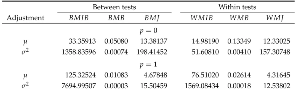
( _s ) . This implies that there are a total of 2,165 observations available for each regression. The resulting estimated response surface coefficients are reported in the top panel of Table 1.

Unreported simulation results suggest that the fit of the response surface regressions can

4Another possibility is to consider maximum eigenvalue type statistics. However, unreported simulation results suggest that the trace statistics perform better in small samples, and we therefore only consider these further.