Impact of renewable energies to European energy systems under historical and future climate conditions

European energy systems under historical and future climate

conditions

Inaugural-Dissertation zur

Erlangung des Doktorgrades

der Mathematisch-Naturwissenschaftlichen Fakultät der Universität zu Köln

vorgelegt von Philipp Henckes

aus Köln

Köln, 2019

Berichterstatter:

Prof. Dr. Susanne Crewell PD Dr. Hendrik Elbern

Tag der Mündlichen Prüfung:

07.06.2019

An meinen Vater, mit dem ich diese letzten Tage meines

Studiums und viele andere Moment gerne geteilt hätte.

Contents

Zusammenfassung 1

Abstract 3

1 Introduction 5

1.1 Climate change risks & the role of variable renewable energy . . . . 5

1.2 Contributions within this thesis . . . . 7

2 Theory 13 2.1 Renewable Energy Output Model . . . . 13

2.1.1 Energy conversion . . . . 13

2.1.2 Model structure . . . . 20

2.2 Clustering algorithm . . . . 23

2.3 Renewable Power System Model . . . . 27

2.3.1 Model Equations . . . . 28

2.3.2 Spatio-temporal resolution . . . . 31

2.3.3 Greenfield mode . . . . 32

2.4 Area potentials . . . . 33

2.4.1 Spatial tessellation . . . . 33

2.4.2 Area restrictions . . . . 34

2.4.3 Area conversion: area power densities . . . . 35

3 Application & data 39 3.1 Generation of a long-term wind power data set . . . . 39

3.1.1 Wind park data . . . . 40

3.1.2 Wind speed data . . . . 42

3.1.3 Energy conversion simulations . . . . 45

3.1.4 Bias correction . . . . 46

3.2 Towards uncertainty estimations for energy system models . . . . . 47

3.2.1 Model chain . . . . 47

3.2.2 Perturbation of wind and PV power . . . . 52

3.3 Simulations of future European energy markets . . . . 55

3.3.1 Wind and solar radiation time series . . . . 56

3.3.2 Setup for the energy system modeling . . . . 63

4 Results 69 4.1 Twenty years of European wind power . . . . 69

4.1.1 Model evaluation . . . . 69

4.1.2 Long-term European wind power . . . . 76

4.1.3 Balancing potentials in Europe and Germany . . . . 80

4.2 Impact of VRE uncertainties to energy system modeling . . . . 83

4.2.1 Error estimation of power output . . . . 83

4.2.2 Sensitivity study . . . . 86

4.2.3 Perturbed VRE power . . . . 88

4.2.4 Impacts on energy systems . . . . 94

4.3 Climate change impact on European energy markets . . . . 99

4.3.1 Future changes of VRE resources . . . . 100

4.3.2 Renewable power production profiles . . . . 105

4.3.3 Impacts on the energy system . . . . 112

5 Conclusions & outlook 121 5.1 Conclusions . . . . 121

5.2 Overall picture and outlook . . . . 125

A Optimal tilt angle of PV systems 129

B Levelized costs of energy 131

C Tables 133

D Figures 141

Bibliography 157

List of Tables 167

List of Figures 169

List of Abbrevations 177

List of Symbols 179

Acknowledgements 183

Erklärung 185

Zusammenfassung

Die Entwicklung des Erdklimas dürfte eine der größten Bedrohungen für Mensch und Natur im 21. Jahrhundert sein, mit kaum vorhersehbaren und im Zweifel auch irreversiblen Folgen für zukünftige Generationen. Daher erscheint es uner- lässlich, dass weltweit versucht wird, die sich abzeichnenden Herausforderungen mit allen verfügbaren Mitteln anzugehen. Erhebliche Veränderungen sind daher nötig, insbesondere im Bereich des Ressourcenmanagements. Der Übergang von fossilen zu erneuerbaren Energien kann dabei eine wichtige Rolle spielen, einen Beitrag zum Klimaschutz durch drastische CO ₂ Reduzierungen zu leisten. Ein Schlüssel ist hierbei, die charakteristischen Eigenschaften der variablen erneuerbaren Energien (VRE) unter gegenwärtigen und zukünftigen kilmatischen Bedingungen besser zu verstehen, um einen neuen Weg in Richtung CO ₂ -freie Energiesysteme und eine insgesamt nachhaltigere Welt einschlagen zu können.

Das damit einhergehende Forschungsfeld ist hochgradig komplex und interdiszi- plinär. Energy Transition and Climate Change, ein Projekt der Universität zu Köln, zielt beispielsweise darauf ab, einen interdisziplinären Rahmen für die Durch- führung verschiedenster Forschungsarbeiten in diesem Bereich zu schaffen, aktuelle Fragen zu beantworten und Neue zu erarbeiten. Die vorliegende Arbeit, als Teil dieses Projekts, profitiert insbesondere vom Wissensaustausch zwischen dem Fach- bereich der Meteorologie und der Wirtschaft. Im Rahmen des Projekts ergeben sich drei Hauptstudien, die sowohl der Dissertation, als auch Teilen von Publikationen dienen.

Studie I zielt darauf ab, die Lücke bezüglich verfügbaren, zuverlässigen und um- fassenden Windenergie-Datensätzen zu schließen, die für sich anschließende Model- lierungen des Energiesystems von Bedeutung sind. Hierfür wird ein neuer Langzeit- datensatz simuliert, der Zeitreihen aller europäischen Windkraftanlagen beinhaltet.

Als Grundlage dient hierbei eine hochauflösende Reanalyse (COSMO-REA6) des Deutschen Wetterdienstes. Hierdurch soll zur Verbesserung und Vertiefung des aktuellen Wissensstands bzgl. der einzigartigen VRE-Merkmale beigetragen und deren mögliche Rolle für Europäische Energiesysteme besser verstanden werden.

Die Analyse der neuen Daten zeigt für Europa und Deutschland eine starke Variabil-

ität der jährlichen Windenergieproduktion, sowie der Auftretenswahrscheinlichkeit

von Extremsituationen. Darüber hinaus deuten die Ergebnisse auf hohe Potentiale

von Ausgleichseffekten innerhalb Europas und insbesondere Deutschland hin. Dies unterstreicht das vielversprechende Potenzial von VRE, um bei der Realisierung einer Europäischen Energiewende zu helfen.

Reanalyseprodukte, wie beispielsweise COSMO-REA6, werden häufig als mete- orologische Grundlage für sich anschließende Energiesystemstudien genutzt, bei de- nen hohe Anteile an VRE Technologien eine Rolle spielen. Da Reanalysen zum Teil erhebliche Fehlerbereiche aufweisen, kommen Fragen nach deren Auswirkungen auf Energiesystem-Modelle auf. Studie II zeigt, dass sowohl die Energieumwandlungs-, als auch Energiesystem-Modelle sehr sensitiv auf Anfangsfehler in den meteorol- ogischen Eingangsdaten reagieren. Das gilt insbesondere bei hohen Anteilen an VRE. In diesem Zusammenhang, können starke Auswirkungen auf die generelle Zusammensetzung des deutschen Stromsystems, sowie Allokationseffekte von VRE- Kapazitäten beobachtet werden. Eine solche Fehleranalyse ist neu im Bereich der Energiesystem-Modellierung.

Schließlich untersucht Studie III die Auswirkungen des Klimawandels auf ein vereinfachtes Europäisches Stromsystem, unter strengen Dekarbonisierungszielen, zum Ende des 21. Jahrhunderts. Dabei liegt der Fokus auf Effekten in Bezug auf VRE-Technologien. Hierfür werden Simulationen durchgeführt und verglichen, die auf historischen und zukünftigen Klimabedingungen basieren. Datengrundlage bilden hier Auszüge aus dem EURO-CORDEX Projekt. Die Simulationen zeigen, dass sich das Gesamtsystem zum Einen an den Klimawandel durch ausgeprägte Verschiebungen der Anteile innerhalb der VRE-Technologien anpasst. Zum An- deren können erhebliche lokale räumliche Verschiebungen von VRE-Kapazitäten beobachtet werden, die das System umsetzt, um die Nachfrage bei gleichzeitiger Erfüllung des CO ₂ -Ziels zu erfüllen. Die Ergebnisse zeigen weiterhin, dass, obwohl die europäischen VRE-Potenziale und ihre Variabilität im Klimawandel-Szenario zu- nimmt, keine wesentlichen Veränderungen im sonstigen Gesamtsystem (Systemkosten, Verhältnis zwischen VRE und Nicht-VRE Kapazitäten, Strompreis) stattfinden.

Diese Anpassungsstrategie verdeutlicht die Notwendigkeit ausreichender Investitio-

nen in Netzkapazitäten, die Dringlichkeit eines gemeinsamen und gemeinschaftlichen

Europäischen Ansatzes als auch entsprechende notwendige Maßnahmen in diesem

Bereich umzusetzen.

Abstract

The development of the Earth’s climate is expected to be one of the greatest threats to mankind and nature in the 21st century, with hardly predictable and perhaps irreversible consequences for future generations. Hence, it appears essential that societies worldwide try to tackle the emerging challenges with all possible means and need to undergo substantial changes, in particular, for resource management.

Energy transition from fossil-based to renewable energies may play a major role contributing to climate change mitigation via drastic CO ₂ reductions. Here, a key is to better understand the variable renewable energies’ (VRE) characteristics for present and future conditions, in order to strike a new path towards CO ₂ -free energy systems and a more sustainable world.

The emerging corresponding research field is highly complex and interdisci- plinary. The Energy Transition and Climate Change project, hosted by the Univer- sity of Cologne, aims to establish an interdisciplinary framework to tackle various research questions as well as to raise new ones. The present thesis is embedded in the project and benefits in particular from the exchange of knowledge between meteorology and economics. Three main studies are related to the project and are subject to this thesis, as well as in parts to publications.

Study I aims to reduce the gap of available, reliable and comprehensive wind power data sets for follow-up investigations by generating a novel long-term Euro- pean wind power time series based on a high resolution reanalysis by the German Weather Service (COSMO-REA6 ). Hereby, the improvement of a comprehensive understanding of the unique VRE power characteristics and their potential role for energy systems in Europe is supported. Analyzing this data base reveals strong vari- ations in annual wind productions as well as of frequencies of extreme situations in Europe and Germany. In addition, results show high potentials of balancing effects within Europe and in particular for Germany, emphasizing the promising potential of VRE to help realizing the energy transition.

Reanalyses products, such as COSMO-REA6, are often used as a meteorological

basis for subsequent energy system studies including high shares of VRE. Since

reanalyses contain considerable biases, the question of their impact to energy system

models arises. Study II shows that energy conversion as well as energy system

models are highly sensitive to initial errors associated with the meteorological input

data, in particular under high shares of VRE. In this context, impacts on the overall composition of German electricity system as well as allocation effects of VRE capacities are observed. Such an uncertainty evaluation is a novelty in energy system modeling.

Finally, Study III investigates the impact of climate change on a simplified Eu-

ropean electricity system under strong decarbonization targets until the end of the

21st century. Here, the focus is on effects with respect to VRE technologies. For

this purpose, simulations based on historical and future climate change scenarios,

under strong CO ₂ emission assumptions, from the EURO-CORDEX project are

compared. Simulations exhibit, that the system on the one hand adapts to cli-

mate change by pronounced shifts within VRE capacities and on the other hand by

substantial local allocation adjustments, in order to fulfill the demand side while

meeting the decarbonization target. The outcomes further show that, although Eu-

ropean VRE potentials decline and their variability increases in the future climate

change scenario, no substantial changes in the overall system (costs, ratio between

VRE and non-VRE, electricity price) can be observed. This adaption strategy em-

phasizes the need for sufficient investments in transmission capacities, the urgency

of a common and joint European approach and corresponding adequate actions

from this day forward.

Chapter 1

Introduction

1.1 Climate change risks & the role of variable re- newable energy

Following the Intergovernmental Penal on Climate Change (IPCC, 2014), one of the biggest challenges and threats for mankind in the 21st century appears to be the change in observed and predicted climate conditions. Numerous recent and ongoing research suggests that climate change leads to consequences concerning many aspects of ecosystems as well as socio-economic related questions and may cause irreversible damage (IPCC, 2014; Tobin et al., 2016). Increased risks of climate change impacts, such as species extinction (Pacifici et al., 2015), ecosystem shifts (Pecl et al., 2017), impairment of human health (Watts et al., 2015), sea level rise (Neumann et al., 2015), intensification of extreme weather events (Forzieri et al., 2016), e.g. heat waves (Schär, 2016), droughts (Teuling, 2018) and floods (Madsen et al., 2014), are to some extent relevant on the global but also on the local scale.

The combination of global economic and population growth in the 20th cen- tury and beyond are estimated to be the main drivers for the large increase in the atmospheric greenhouse gas (GHG) emissions with respect to pre-industrial decades (IPCC, 2011). This leads to the highest concentrations ever observed, mainly for carbon dioxide (CO ₂ ), methane (CH ₄ ) and nitrous oxide (N ₂ O) (IPCC, 2014). While effects assigned to population growth remained constant in recent years, the contribution allocated to economic growth experience a strong enhance- ment. According to the IPCC (2014), it is extremely likely that the increase in anthropogenic GHG emissions represents the dominant cause (more than 50%) of the observed global warming since the mid-20th century (1951-2010). Pervasive sup- ply of energy services has substantially contributed to these historical and present changes in GHG emissions. The IPCC finds that, in particular, fossil fuel combus- tion accounts for the majority of these anthropogenic changes (IPCC, 2014).

A continuing evolution of current GHG emissions is expected to foster further

global warming in the future, leading to associated perseverative changes for all climate system components with an increased likelihood of severe and irreversible impacts and risks for human systems as well as ecosystems (IPCC, 2014). In con- sequence, substantial near future changes, such as sustained pronounced reductions of GHG emissions, are necessary in order to limit future climate change and affili- ated impacts and risks, as claimed for example by the International Energy Agency (IEA, 2011). For instance, a successful realization of the Paris climate agreement ¹ , which aims "to strengthen the global response to the threat of climate change by keeping a global temperature rise this century well below 2 degrees Celsius above pre-industrial levels" appears to be a distant prospect, since under current mitiga- tion ambitions annually averaged global temperature is expected to rise by 2.9 ^◦ C- 3.4 ^◦ C towards the end of the 21st century (in relation to pre-industrial conditions) (IPCC, 2018).

Several recent studies highlight the possibility and various pathways towards fully renewable and sustainable energy systems (Pleßmann et al., 2014; Connolly et al., 2016; Papaefthymiou and Dragoon, 2016), which may potentially contribute to the required adaptions in order to mitigate climate change and its consequences.

Hereby, power generation by variable renewable energy (VRE) technologies, such as wind and solar power plants may play a key role for the mitigation solution (Deng et al., 2012; Connolly and Mathiesen, 2014). Additionally, Bloomberg (2018) mentions that cost-optimal electricity systems are increasingly based on VRE generation technologies, triggered by recent cost reductions of VRE power plants as well as enhanced awareness and regulation of environment related aspects.

VRE based power generation is highly flexible and exhibits pronounced vari- ability on multiple spatio-temporal scales due to the highly variable nature of the associated resources, being near surface wind speed and solar radiation (Perez et al., 2016; Ueckerdt et al., 2015; Monforti et al., 2016; Staffell and Pfenninger, 2016).

Therefore, with rising shares of VRE power supply, the dependency of power pro- duction on weather and climate related aspects increases significantly. Enhanced variability of large parts of the power supply side sharpen the challenge concerning security of supply and system reliability (Lund et al., 2015; Peter and Wagner, 2018). Hence, it appears crucial to understand VRE characteristics on short to long-term scales in order to estimate their potential contribution to an energy tran- sition triggered by policies regarding decarbonization targets. Furthermore, on one hand climate change is a major motivation for large VRE expansions, on the other hand it may influence and alter energy yields from these renewable sources to a

1

At COP 21 in Paris (12 December 2015), the Paris climate agreement emerged within the

international environmental agreement United Nations Framework Convention on Climate Change

(UNFCCC), https://unfccc.int

significant extent in the future. The conservation of the future energy systems’

capability implies an adequate adaptation to changing conditions and, therefore, requires a sophisticated analysis of climate change related effects on these systems (Peter, 2019).

1.2 Contributions within this thesis

The following Sections contain an overview and a detailed introduction to the stud- ies carried out in the scope of this thesis. They aim to contribute to existing research by investigating VRE characteristics under historical and future climate conditions in Europe.

Study I

This study is related to the publication in ENERGY in 2018 with the title "The ben- efit of long-term high resolution wind data for electricity system analysis" (Henckes et al., 2018).

As mentioned before, renewable energies such as wind and photovoltaics (PV) are recently gaining major significance for energy systems world-wide. For example, Europe’s wind capacity increased from 41 GW (6% share) in 2005 to 154 GW (16.7%

share) in 2016 (WindEurope, 2017). To understand and anticipate future energy systems, the VRE contribution and inherent unique characteristics, e.g. short- and long-term variability, have increasing importance. For instance, regarding the reli- ability of energy systems distinct low or high VRE power supply situations play an important role. Low VRE generation cases trigger the need for conventional plants, compensating the missing capacity for a stable demand satisfaction. In contrast, very high VRE supply might lead to increased pressure on the electricity grid, forc- ing transmission system operators (TSOs) to regulate the grid load by powering down certain suppliers. Both cases contribute to additional cost and planning un- certainties for all market participants (Hirth et al., 2015; Wu et al., 2015). A better understanding of the VRE characteristics could reduce these cost and uncertainties to a significant extent. Since wind and solar radiation are spatially highly variable, it is crucial to derive high resolution data for accurate follow-up analyses such as electricity dispatch and investment models, transmission grid expansion or security of supply analyses.

At least two major challenges arise. First, while wind and PV employment ex-

perience rapid expansions, the availability of historical VRE production data for

analyses and predictions are insufficient. Necessary empirical long-term observa- tions of VRE production for large numbers of installed capacities are scarce. Data for individual production sites might be publicly available. However, time series for a high share of the wind and especially PV fleets in an entire country like Germany or even the European Union are unfortunately missing for such analyses and research. Therefore, simulations of VRE time series are required incorporat- ing long-term and high resolution meteorological input with current and expected future wind and PV plant fleets. However, this in turn leads to the second issue.

Historical meteorological observations of wind speed and solar radiation are lacking either high spatio-temporal resolution, the long-term scale or sparse spatial coverage (Staffell and Pfenninger, 2016; Henckes et al., 2018; Cannon et al., 2015). Perform- ing simulations at locations matching exactly with operation sites even complicates the data supply, since observation and production sites usually would not coincide.

A variety of recent studies are applying wind input data from different reanalysis products to tackle these issues (Gunturu and Schlosser, 2012; Cosseron et al., 2013;

Hallgren et al., 2014; Ritter and Deckert, 2017; Staffell and Pfenninger, 2016). They are systematic approaches to generate long-term data sets on a homogeneous grid for climate research by combining assimilation schemes for historical observations with atmospheric circulation models. However, most studies focus only on single countries, reveal comparably low resolutions or lack an advanced level of details, in particular, concerning the energy conversion process. Staffell and Pfenninger (2016) for instance use the Modern-Era Retrospective Analysis (MERRA) by the National Aeronautics and Space Administration (NASA) to model long-term wind power time series in Europe. Besides a sufficiently high temporal resolution (hourly) for VRE related aspects, the MERRA reanalysis has a comparably coarse spatial grid of approximately 50 km in Europe, since sub-grid scale effects might be important to local wind and solar conditions (Liléo et al., 2000; Carvalho et al., 2014).

The work carried out in the scope of this thesis contributes by developing a novel energy conversion model and its application to a unique state-of-the-art reanalysis, bringing along a high spatio-temporal resolution and a long time horizon of 20 years. In combination with a location specific European wind park data set, a high resolved long-term wind power time series is generated on a high level of details.

The resulting database allows to further address the following questions in Study I:

• How is the European wind power characterized? Is it possible to determine a representative wind power year for further investigations?

• How pronounced is the potential of balancing effects related to wind power in

Europe and on a national scale in Germany?

Study II

This study is subject to the article "Uncertainty Estimation of Investment Models under High Shares of Renewables using Reanalysis Data" by Henckes et al. (2019) submitted to ENERGY in April 2019 and will closely follow this work.

As outlined previously, to tackle the issue of the insufficient availability of reliable long-term VRE power production data, many studies are making use of reanaly- sis products serving as the meteorological basis for VRE representation in energy system modeling (Andresen et al., 2015; Bett and Thornton, 2016; Ritter and Deck- ert, 2017). Besides the advantages of reanalyses, questions about effects of their potential errors on modeling outcomes arise.

As it has been observed in many studies (Bollmeyer et al., 2015; Kaiser-Weiss et al., 2015; Staffell and Pfenninger, 2016; Rose and Apt, 2015) and confirmed by this study (Section 3.1.2), reanalysis products show significant uncertainties (e.g. biased) to different extents, depending on the estimated quantity. Staffell and Pfenninger (2016) for instance highlight the urgency for wind power production studies to consider calibration with respect to reanalysis biases. However, when it comes to energy system modeling, these errors are usually omitted (Peter and Wagner, 2018;

Huber et al., 2015; Dolter and Rivers, 2018) and, hence, their potential impact to model results is not considered. The topic gains even more importance for future energy systems, since VRE expansion and shares are expected to strongly increase.

In general, the matter of uncertainties in a sense of error estimation in this field of research appears to leave room for several further investigations and improvements.

Therefore, the approach of this study has the objective to give first insights on potential uncertainties introduced by reanalysis errors and their impact on the affiliated model chain. The approach follows the idea of focusing on the overall range of potential errors rather than quantifying uncertainties of actual real case scenarios. The analyses related to Study II attempts to answer on three main questions:

• What are potential error sources associated with VRE power modeling?

• What are the sensitivities of the applied power conversion models (wind and PV) with respect to these estimated errors? What are the most dominant parameters?

• What are the impacts of these uncertainties on future energy system simula-

tion results regarding the dominant parameters?

Study III

This branch within the framework of this thesis has the objective to comprise the developed methods in order to simulate projections of future energy markets in Europe under high shares of renewable energies. As recent economic and political developments world-wide and, in particular, in Europe reveal, contributions of re- newable energies to the total energy mix will play a central role (e.g. Connolly et al., 2016). With expansion of VRE technologies, however, uncertainties for the energy system increase due to the variable nature of wind and PV energy (Boyle, 2009;

Beaudin et al., 2010; Bessa et al., 2014). In consequence, this leads to stronger challenges regarding energy system related aspects, for instance, security of supply.

At the same time, global climate is expected to go through significant changes in the future, as described earlier. Since these changes might vary essentially between con- tinents or single countries (e.g. IPCC, 2014), some regions could experience strong implications to their potentials of wind and solar related energy generation. As such, the world-wide wind energy potential is expected not to change significantly on average, but climate projections indicate an overall decrease for Europe (e.g. To- bin et al., 2016). In addition, the variability on different time scales is also expected to change, affecting, for instance, the need for conventional backup capacities. With respect to these assumptions, the following question emerges: what is the potential impact of local climate change to the European energy markets?

The topic combines complex processes from various research fields. Therefore the aim of this study is to keep track on the overarching goal to combine mete- orological and economical aspects without getting lost in details and to keep the entire framework as simple as possible in order to focus on the impact of climate change to VRE sources. For instance, various studies examine the impact of climate change on wind or PV energy sources in detail only for single European countries (e.g. Najac, 2014; Nolan et al., 2012; Cradden et al., 2017) or even for the entire European continent (e.g. Reyers et al., 2016; Tobin et al., 2016; Moemken et al., 2018), but would not investigate the subsequent implications for the local energy markets. This has been done by some recent studies, applying future projections from global climate models to energy system modeling (e.g. Tobin et al., 2018; Pe- ter, 2019). However, they concentrate on the economical point of view and try to implement as many details of the entirety of the energy system as possible, while meteorological details are slightly neglected.

This study, in contrast, aims to give first insights on the potential impact of

climate change on Europe with a focus on VRE sources as well as the affiliated

electricity sector. Here, the main objective is to analyze potential future changes

with respect to each step of the necessary model chain in detail – from changes in

wind speeds and solar radiation over their impacts on European VRE potentials to final changes in the European energy system. For this purpose, the modeling approach is kept as simple as possible. By intentionally omitting certain processes and details, the resulting signals are further isolated, so that cause and effect can be related more easily. For instance, climate change might also affect other aspects of the energy systems as pointed out by (e.g. Peter, 2019), such as cooling water avail- ability for thermoelectric power plants (Tobin et al., 2018), hydro power potentials (Schlott et al., 2018) or electricity demand (Wenz et al., 2017).

The overall approach of Study III is to compare future European energy systems under both, present-day climate and future changing climate conditions. For this purpose, VRE time series for both climate conditions are generated by applying the developed energy conversion model to outcomes of global climate model simulations.

By the development and application of a clustering scheme, as well as an energy system model, the impacts of climate change on the European electricity system towards the end of the century are examined.

Structure

Research and analyses within this thesis are closely related to the Energy Transition and Climate Change (ET-CC) project ² , being part of the Institutional Strategy of the University of Cologne funded by the Excellence Initiative. Since the subject of renewable energies with respect to energy transition triggered by future climate changes and their impact on energy markets requires cooperation of various differ- ent research fields and disciplines, the ET-CC project aims to provide an interdis- ciplinary framework, which contributes to relevant ongoing research. Hereby, the objective is not only to work on open research questions, but also to understand the connection between the various participating disciplines and, from this, to address emerging questions concerning renewable energies, energy transition and climate change which can only be answered in close collaboration between, for example, meteorology, economics and informatics. For that matter, the project brings to- gether expertise from various institutions, such as the Institute for Geophysics and Meteorology (IGM) ³ and the Institute of Energy Economics (EWI) ⁴ . With the out- lined studies, this thesis tries to contribute to the projects interdisciplinary research by three major topics:

• Study I: What are the present main characteristics of wind power in Europe and Germany?

2

http://et-cc.uni-koeln.de/project.html

3

http://www.geomet.uni-koeln.de/home/

4

http://www.ewi.uni-koeln.de/

• Study II: What is the impact of VRE uncertainties on outcomes of energy system models?

• Study III: What are the climate change impacts on European energy markets by the end of the 21st century under high shares of VRE?.

All three investigations share and apply parts of tools and methods developed

and described in Chapter 2. Chapter 3 outlines the combination and application

of these tools and methods as well as the necessary input data sets used for the

respective study. This is followed by Chapter 4, describing the respective results

for Studies I-III. Chapter 5 concludes with a discussion of the emerging results and

provides an outlook.

Chapter 2

Theory

2.1 Renewable Energy Output Model

In the scope of this thesis, the Renewable Energy Output Model (REOM) is devel- oped: A tool which creates historical and future VRE power production data sets for given wind speed and radiation data and installed plant capacities in a certain domain. Applying the model to high resolution input data sets such as meteorolog- ical reanalysis fileds yields spatially and temporally accurate VRE generation time series. Section 3.1.2 discusses reanalysis data sets in detail. REOM is highly flexible at any stage of transition from input resource quantity, i.e. wind speed and solar radiation, to the actual power generation output by a certain power plant fleet.

For instance, it is possible to switch between different interpolation schemes or to choose the level of details considered for the calculations. Another key feature of the model is the ability to handle any level of spatial and temporal resolution. The following Sections 2.1.1-2.1.2 depict the model Equations, structure and different settings as well as all crucial details of REOM.

2.1.1 Energy conversion

The REOM model core incorporates one wind and one PV model to derive the conversion from the environmental quantity to electrical power supply of a given plant facility. These are processed for every plant and time step contained in the simulation.

Wind model

Following Henckes et al. (2018), the power output P out of a single wind turbine at

a known location for given instantaneous wind speeds at hub height v _hub is derived

by the Equation 2.1, also called power curve:

P _out =



 

 

 

 

 

 

 

 

 

 

0, v hub < v in , 1

2 πR ² c _p ρ _hub · v ³ _hub , v _in ≤ v _hub < v _r , C _plant , v _r ≤ v _hub < v _out ,

0, v _hub ≥ v _out .

(2.1)

On the meteorological side, the power output depends on the wind speed v _hub and air density ρ hub at hub height of the rotor. The rotor diameter R, efficiency c p , capacity C _plant , cut-in wind speed v _in , cut-out wind speed v _out as well as rated wind speed v _r are determined by the specific turbine type. Equation 2.1 shows that a wind turbine produces energy as long as wind speeds at turbine hub height v _hub range between the cut-in and cut-out point. With wind speeds higher than the rated speed v _r this is accomplished at a maximum rate – the capacity of the turbine.

Between cut-in and rated speed the power production is mainly proportional to the cubic wind speed at hub height. Below v _in the unit would not produce any power due to the mechanical inertia of the turbine. Also, it stops for wind speeds higher than v out due to technical limitations and security issues.

Due to the cubic dependency of the power output to the wind speed at hub height in Equation (2.1), it is crucial to have highly accurate wind input data.

The wind input data is obtained on a consistent grid defined by the meteorological input data set. As the grid points on the horizontal and vertical level usually do not coincide with the wind park position and hub height, three steps are necessary to get the wind speed at the specific turbine spot. First of all, the absolute values at each grid point need to be calculated from the horizontal components vx and vy of a gridded wind field by

v _i,j,k = ^q vx ² _i,j,k + vy ² _i,j,k

i = 1, ..., m j = 1, ..., n k = 1, ..., p

(2.2)

where i, j and k are the grid points in x, y and z-direction. As a second step the

absolute wind speeds are horizontally interpolated from adjacent grid points to the

exact specific turbine or wind park location. Different interpolation schemes are

offered in REOM. Beside a bilinear interpolation, the inverse distance weighting

method (IDW) is featured. For the studies designed in Sections 3.1-3.3 the latter

is applied – accounting for the exact distance of the known grid point values to the

unknown wind park location values, using distance weights. The interpolated wind

speed v at point P is given by

v(p) =



 



 

 P N

i=1 w(p _i ) · v (p _i )

P _N

i=1 w(p i ) , d(p, p i ) 6= 0 v(p _i ) , d(p, p _i ) = 0

(2.3)

with

d(p, p _i ) = ^q (p _x − p _x,i ) ² + (p _y − p _y,i ) ²

being the distance between the interpolation point p and the gridded sampling points p _i . The corresponding weight is expressed by

w = d(p, p _i ) ^−ζ

where ζ, the power parameter, is set to 2.

Finally the horizontally interpolated wind speeds need to be vertically interpo- lated, respectively extrapolated to the adjacent hub height. This can be obtained in various ways. The two most common approaches apply the logarithmic wind profile or the Hellmann exponential law (power law) to extrapolate near surface (e.g. 2 m or 10 m) wind speeds to the desired height (Andresen et al., 2015; Hueg- ing et al., 2012; Reyers et al., 2016; Tobin et al., 2014). The vertical wind profile may only in some cases follow a logarithmic profile depending, for instance, on the atmospheric stability conditions. A resulting disadvantage is therefore the inher- ent inability to reproduce the vertical wind profile at any time and time scale due to different prevailing atmospheric stability conditions (Stull, 1988; Kaimal and Finnigan, 1994; Motta et al., 2005). Extending the logarithmic profile by stability correction terms would be a possible solution to this problem (Stull, 1988; Manwell et al., 2009; Rose and Apt, 2015). However, in addition to the wind fields, several other variables would be necessary to account for atmospheric stability, increasing the model complexity significantly (Stull, 1988). The second approach, the power law, is widely used for engineering and wind energy applications due to its mathe- matical simplicity: the ratio between the wind speed v _hub at hub height and v _ref at a reference height near the surface are equal to the ratio of these heights raised to the power of the Hellmann exponent α:

v _hub = v _ref ·

z _hub z _ref

α

(2.4)

According to Emeis and Turk (2007), Equation 2.4 offers a nearly perfect fit to the

corrected logarithmic wind profile under stable conditions for certain surface rough-

ness conditions and a good approximation under neutral and unstable conditions

in the limit of very smooth surfaces. REOM features both extrapolation schemes, bringing along the advantage of moderate input data requirements (e.g. only one level of 2-dimensional wind speeds necessary). As a third option, REOM offers the possibility to use a vertical interpolation between different wind speeds at different model layers obtained from the input data set. For this purpose, wind speeds of the first vertical levels are taken as sampling points for a 3rd order fit, which is used for an interpolation from the closest level to the actual hub height. Certainly, in order to apply the latter scheme the meteorological input data set needs to contain vertical resolved wind speed data.

PV model

Following Quaschning (2011) the ideal power output of a PV module P out,ideal can be estimated by the product of the module’s area A _mod , efficiency η and the global solar radiation on a tilted plane G ^tilt _tot :

P _out,ideal = A _mod · η · G ^tilt _tot . (2.5)

Due to various effects of energy loss, the power yield of a PV module is actually lower in reality as depicted in Equation 2.5. Amongst others, Quaschning (2011) mentions the following effects contributing to the power loss:

• efficiency decline due to module warming and part load operation,

• reflection losses,

• change of efficiency due to spectral effects,

• soiling and snow,

• shading,

• conduction and diode losses.

Thus the so called performance ratio of a PV module P _r is implemented to yield the real power output P out,real :

P _out,real = P _r · P _out,ideal . (2.6)

Multiplication of the module area by the efficiency η _STC of the module at Standard Test Conditions (STC) and the global solar radiation G ^tilt _STC yields the theoretical capacity of the module C:

C = A _mod · η _STC · G ^tilt _STC

Equations 2.5 and 2.6 can then be rearranged to P _out,real = P _r ·



 C · η

η _STC · G ^tilt _tot G ^tilt _STC



 (2.7)

The efficiency η depends on the module’s actual temperature T _mod and the temper- ature at Standard Test Conditions T _STC (Mack et al., 2013):

η = η STC ·

1 − β T mod − T STC

(2.8) where β is the temperature coefficient in units of ^◦ C ⁻¹ . In Equation 2.8 it describes the loss in efficiency, and hence power loss, the module is facing per ^◦ C increase in temperature. T _mod is a function of the global solar radiation on the tilted plane and the ambient air temperature T 2m and given by:

T _mod = T _2m + c _T · G ^tilt _tot

G ^tilt _STC (2.9)

The proportionality factor c T is a constant temperature and depends on the specific location of the PV module – ranging from 22 ^◦ C for complete elevation free spots to 55 ^◦ C for facade integrated non-ventilated solutions (Quaschning, 2011). It can be seen as the temperature surplus the module faces compared to the STC case (Equation 2.9). Actually c _T depends on the ambient wind speed accounting for a cooling of the module by the wind. For simplicity and the fact that the local situation and specific module characteristics are often unknown in large PV facility data sets, the same c _T is set for all data set members.

Finally, Equation 2.7 requires the feed-in of the global solar radiation G ^tilt _tot on the tilted plane, which is defined by the sum of the two solar radiation compo- nents, direct G ^tilt _dir and diffuse G ^tilt _dif , as well as a part reflected by the surface G ^tilt _ref (Quaschning, 2011).

G ^tilt _tot = G ^tilt _dir + G ^tilt _dif + G ^tilt _ref (2.10) First, the direct radiation on the tilted plane in Equation 2.10 can be calculated given the direct solar horizontal radiation G ^hor _dir , an estimate of the solar incident angle on the tilted plane Θ _tilt as well as the actual sun’s zenith angle γ _s :

G ^tilt _dir = G ^hor _dir · cos Θ _tilt

sin γ _s (2.11)

The incident angle on the tilted plane can be estimated by using the sun’s zenith

γ _s and azimuth angle α _s as well as the module’s tilt angle γ _m and azimuth angle

α _m :

Θ _tilt = arccos − cos γ _s sin γ _m cos (α _s − α _m ) + sin γ _s cos γ _m

Second, the estimation of the diffuse fraction on a tilted plane in Equation 2.10 is more complex than for the direct part. According to Quaschning (2011) an anisotropic approach reveals significantly increased accuracy in contrast to the rather simple isotropic ones. They take into account that the radiation density might vary substantially with different cardinal directions, in particular for clear- sky cases. In Chapter 3, two different anisotropic schemes are applied and compared – one approach by Klucher (1979) and one by Perez et al. (1986). For the Klucher model (KM), the diffuse solar radiation on a tilted plane is derived by:

G ^tilt _dif = G ^hor _dif · 1 2

1 + cos γ _m 1 + F sin ³ γ _m 2

1 + F cos ² Θ _tilt cos ³ γ _s (2.12) with

F = 1 −





G ^hor _dif G ^hor _tot





2

.

The more accurate but also more computationally expensive approach compared to Equation 2.12, is the Perez model (PM). First of all, the clear-sky index and the lightness index ∆ are derived:

=





G ^hor _dif + G ^hor _dir sin ⁻¹ γ _s

G ^hor _dif + κ · Θ ³ _hor







 1 + κ · Θ ³ _hor





−1

(2.13)

∆ = G ^hor _dif sin γ s · E 0

(2.14) with the constant κ = 1.041, the incident angle on the horizontal plane Θ _hor and the solar constant E ₀ . By using Equations 2.13 and 2.14, both, the lightness index for the horizon and for the sun’s near ambience, can be calculated:

F ₁ = F ₁₁ () + F ₁₂ () · ∆ + F ₁₃ () · Θ _hor

F ₂ = F ₂₁ () + F ₂₂ () · ∆ + F ₂₃ () · Θ _hor (2.15) The constants F ₁₁ -F ₂₃ in Equations 2.15 are assembled in the Appendix, Table C.1. Here, Perez et al. (1986) distinguish between eight different clear-sky classes.

Finally, the indices F ₁ and F ₂ as well as

a = max (0; cos Θ _tilt )

b = max (0.087; sin γ _s )

yield the diffuse solar radiation on the tilted plane:

G ^tilt _dif = G ^hor _dif ·

1

2 (1 + cos γ _m )(1 − F ₁ ) + a

b · F ₁ + sin γ _m · F ₂

(2.16) Since analyses in Chapter 3 show that the differences between the schemes of KM and PM are neglectable concerning long-term energy production simulations and by comparing their complexity, only the KM is implemented in REOM and used for upcoming simulations.

Third, for the reflected solar radiation on the tilted plane G ^tilt _ref in Equation 2.10, an isotropic approach is sufficiently accurate:

G ^tilt _ref = G ^hor _tot · α _sfc · 1 2

1 − cos γ _m . (2.17)

The surface albedo α _sfc is defined as the ratio of reflected radiation to the received radiation by the surface. Therefore, it’s dimensionless value is determined by the surface type and characteristics and ranges between 0.05 for certain forests and up to 0.9 for fresh snow covers. If the surface type, and hence albedo, in the vicinity of the PV module is unknown a value of 0.2 is commonly set over land.

Many available meteorological data sets only supply the total solar radiation on a horizontal plane G ^hor _tot . However, to derive the total solar radiation on a tilted plane required in Equation 2.7, it is necessary to differentiate into direct and diffuse radiation parts (see Equations 2.11, 2.12 & 2.16). This can be accomplished using statistical relations (Quaschning, 2011). Using hourly values of G ^hor _tot and the solar constant E ₀ as well as the sun’s zenith angle γ _s , the factor k _T in Equation 2.18 can be derived by

k _T = G ^hor _tot E ₀ · sin γ _s .

The diffuse and direct fractions are then estimated applying Equations 2.18 and 2.19:

G ^hor _dif =



 

 



 

 



G ^hor _tot · 1.020 − 0.254 · k _T + 0.0123 · sin γ _s , k _T ≤ 0.3 G ^hor _tot · 1.400 − 1.749 · k _T + 0.177 · sin γ _s , 0.3 < k _T < 0.78 G ^hor _tot · 0.486 · k _T − 0.182 · sin γ _s , k _T ≥ 0.78

(2.18)

G ^hor _dir = G ^hor _tot − G ^hor _dif (2.19)

To obtain radiation time series at all operation sites, the values incorporated in

the meteorological data set need to be interpolated from the underlying grid to the

specific locations. This is processed equivalent to the previously discussed wind

model.

2.1.2 Model structure

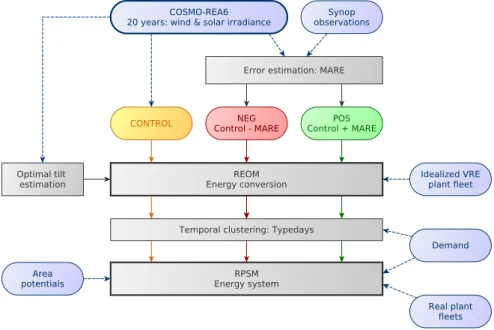
As illustrated in Figure 2.1, REOM consists of five main modules, namely CAPS, GEO, FIELDS, INTP and ENERGY. A central configuration file controls which modules to run as well as all input and simulation settings. The former three modules gather and assimilate input data and settings, in INTP variables are inter- polated and extrapolated, and ENERGY builds the actual REOM core processing the energy conversion.

Figure 2.1: Schematic illustration of the REOM model.

CAPS

This module prepares all necessary information for the VRE plant fleets as out-

lined in Section 2.1.1. These include site coordinates, altitudes and locations (on-

shore/offshore), commission dates (date when a plant started to produce power)

and total capacity as well as the manufacturer and plant type. In addition, specific

turbine characteristics like rotor hub height and diameter, cut-in, cut-out and rated

wind speed are assembled in case of wind parks. Whereas in case of PV plants,

plane tilt and azimuth angle are set as well as the module’s specific temperature

factor, performance ratio, efficiency and temperature at Standard Test Conditions

(STC). For all plant specific characteristics, it is possible to determine whether an existing data base or constant values are processed. Furthermore, REOM provides different handling options for missing data, i.e. whether to take average values or predefined constants. As part of the country loop, CAPS provides information and characteristics of every individual VRE operation site for all countries set in the configuration file.

GEO

In GEO the domain, geographical and meteorological 2-D fields are imported and processed for every country. For instance, the meteorological grid is coupled to the boundaries of participating countries to reduce all following input fields to the required domain. Surface altitude, albedo and the vertical coordinate are also read from the meteorological data set.

FIELDS

The next step is to read and prepare all the meteorological 2-D and or 3-D fields of all required variables. These include the wind speed, surface temperature and solar radiation. Depending on the chosen meteorological data set and vertical ex- trapolation scheme, the wind components of either only the first or the first five vertical levels is read. Using Equation 2.2 yields the wind speed time series. In case of radiation, the input data set determines whether the global horizontal solar radi- ation on the horizontal plane is processed or the two components separately, being direct and diffuse radiation. The configuration file determines the time horizon for which REOM simulates the energy output. Hence, all variables are extracted for the defined time period and spatial domain (including all countries).

INTP

For both, the wind and solar radiation resource INTP interpolates the variables hor- izontally from the meteorological grid to all operational sites using the interpolation scheme according to the configuration file. In case of wind, a vertical extrapolation scheme is applied afterwards yielding the wind speed at required hub heights.

Depending on the availability of the solar radiation quantities in the meteoro-

logical data set, Equations 2.12 and 2.11 might be applied to separate the radiation

fractions from the global solar radiation. Since radiation is so far referred to a hori-

zontal plane, the KM is used for the conversion to a tilted plane. This is followed by

derivations of the reflected part applying Equation 2.17 (incorporating the surface

albedo) and finally the global solar radiation on the tilted plane via Equation 2.10.

ENERGY

This module is the main core of REOM since the conversion from the meteorological resource to power output by a power plant is processed. For wind, the power curve relation (Equation 2.1) is applied, whereas Equations 2.7-2.9 are used to model PV modules.

REOM offers the option to run a simulation in "live" or "fixed" mode (set in the configuration file). The former means that the actual commission dates are taken into account – for all time steps prior to the commission date of a plant the power output is set to zero. In contrast, when the model runs in "fixed" mode, a reference date is predefined in the configuration file by the user. In this case, only outputs of plants which started prior to that reference date are taken into account. Therefore, in "fixed" mode the plant fleet is the same for any given time step in the simulation.

This is very useful when different time steps or periods are compared, e.g. if the question is whether 1995 was a rather good or bad VRE year compared to other years: Since in 1995 there were almost no wind parks or PV plants installed in the European Union (EU) compared to, e.g. 2014, the "live" mode would not be able to generate comparable years.

Finally, the outcome of a full REOM simulation contains VRE (wind and PV) output time series for each operation site in the pre-defined spatial domain and for the entire time period. Both, the maximum spatial and temporal resolution is determined by the meteorological input data set, but might be decreased by the user. REOM writes output files on a daily, monthly or yearly basis and for each country separately. The model is implemented in MATLAB ¹ and is able to run in MATLAB’s parallel mode (country loop).

As a very last step, the power production time series is converted to a time series of so called capacity factors (CF). This quantity is obtained by normalizing the total sum of power production P of an operation site at all time steps t with its capacity value C multiplied by the respective considered time period ∆t:

CF =

P

t P _t C · ∆t .

The capacity factor is unitless (mostly given in %) and can be interpreted as a measure of the efficiency and capacity utilization of a power plant. Hence it is a very useful parameter for comparisons of different plants as well as different power production technologies. Typically, investigations deal with yearly production val- ues, which gives rise to another quantity of interest – the so called full load hours

1

MATLAB is developed by MathWorks. In the first place it is a numerical computing environ-

ment and programming language. www.mathworks.com

(FLH). The FLH value of an operation site estimates how many hours the facility theoretically has to be operated at full capacity to gain the same annual power yield: the capacity factor is simply multiplied by 8760 h to obtain the FLH of an operation site. In conclusion, both parameters supply the same information.

2.2 Clustering algorithm

To model an energy market system for one entire year, the system of Equations (e.g.

see Section 2.3) is fed with time series of wind and PV energy as well as demand – for example, with an hourly resolution that would lead to three times 8760 of data points. Investment models often even simulate time periods of several years or decades, increasing the amount of data and hence set of Equations dramatically.

Applied to these kinds of systems, even a very simplified investment model would need high amounts of computational costs. Therefore, in many cases it is crucial to reduce the dimensions of the model (set of Equations). This can be accomplished by decreasing the spatial and or temporal resolution of the VRE input data. For instance, the resolution within a day can be reduced to 3, 6 or even 12h. Regarding the spatial dimension, an option would be to decrease the number of horizontal grid points taken into account. However, in many cases these solutions might not be effective enough. In addition, in most of the studies, wind and PV time series are even accumulated for an entire country (e.g. Gils et al., 2017; Dominković et al., 2016; Cebulla et al., 2017). This might have a great impact on the computational costs but at the same time significant uncertainties might be introduced concerning VRE profiles due to the coarse accumulation step.

Hence the objective is to reduce the complexity of the system and at the same time not to loose too much information regarding important characteristics con- tained in the original input data. One way to tackle these problems is the appli- cation of cluster algorithms (Merrick, 2016). Such an algorithm tries to find a set of unique clusters (characteristic subsets) inside the complete data set, containing data points or time series (e.g. days) as similar as possible. In other words, the complete data set is divided into groups with members of similar characteristics.

As a next step, one representative data point or time series needs to be derived from each cluster. For instance, this can be the average of a cluster or one specific cluster member.

In the scope of this thesis, cluster methods are developed for either, the spatial

and temporal scale as well as a combination of these. Figure 2.2 illustrates the

implemented method depicted in detail in the following. The spatial clustering is

supplied by a VRE time series with certain locations and for a defined time period.

Figure 2.2: Schematic illustration of the clustering method and its pathways.

As an output of REOM, a VRE matrix would usually have the dimensions:

N _locations × N _days × N _hours .

To process the algorithm, it needs to be reshaped so that the locations are still represented by the rows (cluster dimension) and the time steps by the columns:

N _locations × N _days · N _hours .

The output of the clustering algorithm will be characteristic and unique groups or clusters of locations which are similar to each other, i.e. a set of representative regions. Note that the spatial clustering is applied separately for different VRE sources – leading to potential differences in the regional partitioning concerning wind and PV energy.

Concerning temporal clustering, the wind and PV as well as the energy demand

time series need to be merged in a first step as the characteristics of each time step

are depending on all three quantities in energy system modeling. Similar to the

spatial case, a reshape of the clustering matrix is necessary. In order to generate typical characteristical days (from now on called typedays), the day-dimension is object to the clustering algorithm. Therefore, this time rows represent days, leading to the following matrix:

N _days × N _locations · N _hours · 3 .

Note that the number of 3 appears due to the three time series merged in the beginning. As a last step, the output matrix needs to be separated again yielding diurnal time series for wind, PV and demand respectively. In other words, the temporal clustering generates distinct typedays containing diurnal profiles of all three quantities.

The clustering routine is developed in MATLAB and provides, as indicated in Figure 2.2, three pathways:

i. temporal clustering only −→ full location grid & typedays, ii. spatial clustering only −→ region cluster & entire time series, iii. spatial & temporal clustering −→ region cluster & typedays.

For the latter, the output of the spatial clustering step is serving as an input for the temporal clustering. In all cases, the actual algorithm can be selected between ward and k-means (MATLAB functions "ward" and "k-means"). They are set to use the Euclidean distance as a measure and, in case of k-means, a maximum of 100 iterations is chosen. Both schemes provide the possibility to pre-define the actual number of clusters (i.e. typedays or regions). Therefore, the clustering routine offers two options – using either fixed cluster numbers or identifying the optimal cluster numbers (only valid for spatial clustering). The latter is implemented by evaluating the silhouette scores while iterating the number of clusters (MATLAB function "eval"). The higher the score, the closer to the optimal number of clusters.

As mentioned before, the developed routine provides two ways of extracting a representative R of each cluster c, namely "average" and "closest". The former takes the mean of N cluster members M :

R _c = 1 N _c ·

N

X

i=1

M _i , for c = 1, ..., N _cluster .

whereas for the second way the most similar cluster member M to the cluster mean µ is determined by an estimation of the minimum of the standard deviation:

R _c = min



 v u u u t

N

X

j=1

(M _j − µ _c ) ² N c



 , for c = 1, ..., N _cluster

An advantage of the latter is that it keeps the inherent variability of the time series, in contrast to a damping due to the averaging process.

Furthermore, the routine checks for the feasibility of the system – is a sample size too small, the entire sample is considered as one cluster. This becomes essential for the spatial clustering, since certain smaller domains (in combination with the spatial resolution) contain only a few grid points. For instance, a country like Luxembourg and a horizontal resolution of 44 km (as in Section 3.3) provides only two sample points for the routine. Hence the clustering looses its classical meaning.

In this example, only one region is assigned to Luxembourg consisting of all grid points in the country. The feasibility is given when

k-means: sample size N cluster

> 2 and ward: sample size ≥ 2

.

Comparing the characteristics of a set of clusters with its original data set some- times shows significant deviations, even for the mean of the quantity. Obviously this can be a problem, e.g. concerning the overall level of energy production of a VRE quantity in a specific region or country. Therefore, after all a scaling process is implemented in the end of the clustering routine to ensure that the production levels are at a similar magnitude in the set of cluster representatives CF clust and the original data CF _orig . This is accomplished by a comparison of mean values in both data sets yielding a factor f

f = mean(CF _orig ) mean(CF _clust ) . which is then used to scale the cluster representatives:

CF ⁰ _clust = CF _clust · f,

CF ⁰ _clust (CF ⁰ _clust > 1) = 1.

The scaling might generate capacity factors greater than 1, a 100% capacity utiliza- tion, which is obviously impossible and therefore corrected. The scaling is iterated until the factor is converging to 1 within a pre-defined precision range p r (e.g.

p = 0.001):

1 − p _r < f < 1 + p _r .

The final output of the clustering routine is a set of cluster representatives (either regions, typedays or a combination of both) with the aim to capture the main characteristics of the original data set while realistically representing the overall level of energy production rates as well as demand levels. To be able to reconstruct the original data set or parts of it, the output is complemented by the occurrence frequencies of each cluster. For instance, to generate one year of VRE production and demand from a typeday data set, the respective occurrence frequency needs to be applied to each typeday and the result multiplied by the number of days, in this case 365.

2.3 Renewable Power System Model

Given a system of various power generating technologies, each with different char- acteristics such as fuel costs, efficiency or carbon dioxide (CO ₂ ) emissions, and a determined power demand: what would be the favorable composition of capacity assets to be able to serve the demand at minimum costs for every time step in a certain period of time? This question implies that a sort of optimization is neces- sary to solve the problem, i.e. a minimization of costs under certain assumptions and constraints. Numerous optimization models were developed to tackle similar problems – some more complex than others, depending on the exact objective and research question.

Such an optimization model is developed to approach the specific problems of

this thesis. From now on, this model is called Renewable Power System model

(RPSM). Compared to other investment models used for energy system studies,

the RPSM is in most parts a rather simple model since it lacks some characteristics

of a realistic reproduction of the energy market system. For instance, the RPSM

only considers the electricity sector of the energy system, ignoring that energy in

the form of heat might play a major role as well. Also the electricity net within a

country as well as storage and diversified plant technologies are neglected. However,

the energy system model is kept to a lower complexity on purpose to be able to

isolate crucial processes for an easier interpretation of the outcomes.

2.3.1 Model Equations

The RPSM core contains a linear programming model, which minimizes the overall costs of the energy system for a certain domain and time period. It is considered a perfect foresight model – the optimization scheme knows all relevant information as well as future processes and developments are anticipated. For example, the model might decide to invest in a certain asset in the beginning of the time period due to the knowledge of future needs.

The main Equation – in linear optimization also called objective function – in the RPSM, which needs to be minimized, is the total sum of all costs C in the system arising from all regions R, technologies T and time steps (years) Y :

min C = ^X

r∈R

X

t∈T

X

y∈Y

C _r,t,y ^inv + C _r,t,y ^fix + C _r,t,y ^var

(2.20) where

C _r,t,y ^inv = P _r,t,y ^add · c ^inv _t,y , (2.21)

C _r,t,y ^fix = P _r,t,y ^exi · c ^fix _t,y · dt _y , (2.22)

C _r,t,y ^var = ^X

d∈D

X

h∈H

G _r,t,y,d,h · c ^var _t,y · f _d · dt _y · τ · 365. (2.23) The investment costs C ^inv are determined by the product of the technology specific investment costs c ^inv and the total amount of capacities added to the system P ^add (Equation 2.21). Similarly, fixed costs for operation and maintenance (FOM) C ^fix of the assets are derived by multiplying the existing installed capacities of a technology at a time step by its specific FOM costs c ^fix (Equation 2.22). Since FOM costs are usually given per year, the amount of years between two simulation time steps need to be considered here (dt _y = Y (y) − Y (y − 1)). In contrast, the so called variable costs C ^var are the total sum of generation costs composed of the power generation G of a technology and the associated fuel costs c ^var (Equation 2.23).

In the first place, this product is calculated for all time steps (for more details on time steps see Section 2.3.2), however in case of applying typedays (see Section 2.2) an upscaling towards an entire year of production is derived with the typeday occurrence frequencies during a year f _d , the amount of days in a year and the hourly resolution τ .

All regional installed existing capacities P ^exi of each technology and time step

consist of the installed capacities from the last time step y − 1, which can be

complemented by additional capacities P ^add or subtractive capacities P ^sub by the