Ab initio studies of extrinsic spin-orbit coupling effects in graphene and quantum Monte Carlo simulations of phosphorene

Ab initio studies of extrinsic

spin-orbit coupling effects in graphene and quantum Monte Carlo simulations of

phosphorene

DISSERTATION

zur Erlangung des Doktorgrades der Naturwissenschaften (Dr. rer. nat.)

der Fakult¨at f¨ ur Physik der Universit¨at Regensburg

vorgelegt von

Tobias Frank

aus Regensburg

im Jahr 2018

Die Arbeit wurde angeleitet von: Prof. Dr. Jaroslav Fabian Pr¨ ufungsausschuss:

Vorsitzender: Prof. Dr. Jascha Repp Erstgutachter: Prof. Dr. Jaroslav Fabian Zweitgutachter: Prof. Dr. Ferdinand Evers

(im Kolloquium vertreten durch: Prof. Dr. Milena Grifoni) weiterer Pr¨ ufer: Prof. Dr. Gunnar Bali

(im Kolloquium vertreten durch: Prof. Dr. Vladimir Braun)

Termin Promotionskolloquium: 12.02.2019

Contents

Notation vii

1 Introduction 1

2 Theoretical foundations and methodologies 3

2.1 Overview . . . . 3

2.2 Density functional theory . . . . 5

2.2.1 Nonrelativistic density functional theory . . . . 5

2.2.2 Exchange and correlation functionals and correction schemes . . 9

2.2.3 Projector augmented wave method . . . . 12

2.3 Effects from the relativistic kinetic energy . . . . 18

2.3.1 Single-particle Dirac equation . . . . 18

2.3.2 Nonrelativistic limit of the Dirac equation . . . . 19

2.4 Relativistic spin density functional theory . . . . 21

2.5 Quantum Monte Carlo . . . . 23

2.5.1 Variational Monte Carlo . . . . 24

2.5.2 Trial wave functions . . . . 26

2.5.3 Diffusion Monte Carlo . . . . 28

2.6 Employed Programs . . . . 33

3 Copper adatoms on graphene: theory of orbital and spin-orbital effects 35

3.1 Extrinsic effects of spin-orbit coupling in graphene due to adsorbates . 35 3.2 Computational methods and system geometries . . . . 37

3.2.1 Methods . . . . 38

3.2.2 Absorption sites and structural relaxation . . . . 38

3.2.3 Error estimation for spin-orbit coupling in the copper atom . . . 39

3.3 Electronic structure . . . . 41

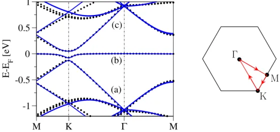
3.3.1 Copper in the top position . . . . 41

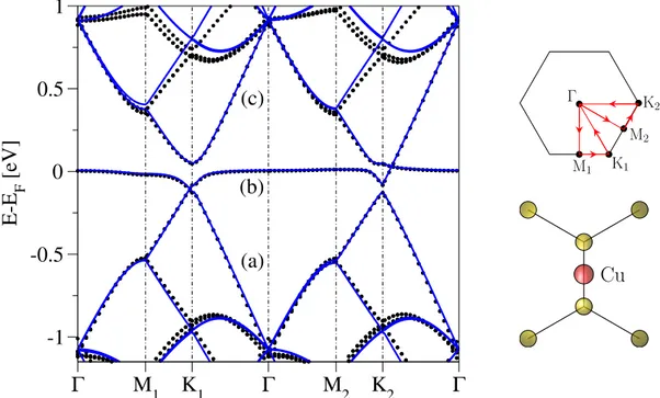
3.3.2 Copper in the bridge position . . . . 43

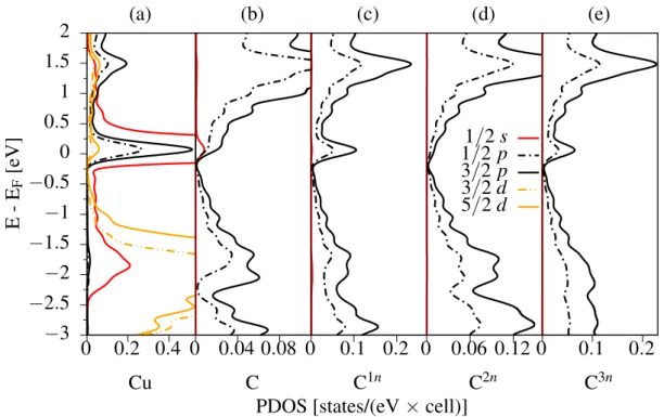
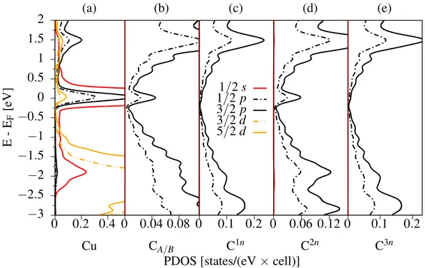
3.3.3 Origin of the local spin-orbit coupling . . . . 46

3.3.4 Spatial visualization of spin-orbit coupling . . . . 50

3.4 Tight-binding models and extraction of spin-orbit coupling parameters 50 3.4.1 Top configuration . . . . 52

3.4.2 Bridge configuration . . . . 55

3.5 Summary and conclusions . . . . 58

4 Theory of electronic and spin-orbit proximity effects in graphene on Cu(111) 59

4.1 The hybrid system graphene–Cu(111) . . . . 59

4.2 Computational methods . . . . 60

4.3 Choice of simulation geometry . . . . 61

4.4 Electronic structure and comparison with photoemission experiments . 63 4.5 Graphene proximity model Hamiltonian . . . . 66

4.6 Parameter extraction and validation of the model . . . . 69

4.7 Graphene–copper distance study of proximity parameters . . . . 71

4.7.1 Geometry dependence of intrinsic spin-orbit coupling . . . . 74

4.7.2 Staggered potential sign change . . . . 76

4.8 Summary and conclusions . . . . 78

5 Protected pseudohelical edge states in Z2-trivial spin-orbit coupling proximitized graphene 81

5.1 Topological states and proximity effects in graphene . . . . 81

5.2 Graphene spin-orbit coupling proximitized tight-binding Hamiltonian . 84 5.3 Ribbon physics: a comparison between the quantum spin Hall effect and sublattice-broken spin-orbit coupling systems . . . . 85

5.3.1 Special cases of intrinsic spin-orbit couplings . . . . 85

5.3.2 Zigzag band structures . . . . 85

5.3.3 Armchair band structures . . . . 89

5.4 Topological classification . . . . 91

5.4.1 Intrinsic spin-orbit coupling phase space: bulk gap and topo- logical invariant . . . . 91

5.4.2 Bulk low-energy band structure shapes . . . . 92

5.4.3 Berry curvature in the staggered spin-orbit coupling case . . . . 93

5.5 Ribbon width effects and finite flakes . . . . 95

5.5.1 Zigzag edge state localization properties . . . . 95

5.5.2 Protected pseudohelical edge states . . . . 95

5.5.3 Condition for the absence of valley edge states . . . . 98

5.5.4 Emergence of pseudohelical states in finite flakes . . . 100

5.6 Effect of uniform onsite disorder on edge states . . . 101

5.7 Summary and conclusions . . . 103

6 Many-body quantum Monte Carlo study of phosphorene 105

6.1 Introduction to phosphorene . . . 105

6.2 Fundamental gap . . . 109

6.3 Phosphorene lattice . . . 112

6.4 DFT electronic structure . . . 113

6.5 QMC for periodic phosphorene . . . 114

6.5.1 Trial wave function . . . 117

6.5.2 Trial wave function optimization . . . 121

6.5.3 Data correlation and statistical error estimation . . . 122

6.5.4 Supercell dependence of the ground and excited state energy . . 124

6.5.5 Cohesive energy . . . 126

6.6 QMC for phosphorene clusters . . . 128

6.7 Fundamental gap from periodic and cluster QMC calculations . . . 129

6.8 Interpretation in terms of experiments . . . 133

6.9 Summary and conclusions . . . 134

Contents

A Numerical evaluation of the topological Z2 invariant with Z2Pack 137 B Symmetry classification of graphene proximity Hamiltonians 143 C Degeneracies of graphene proximity Hamiltonians at the K point 147

D Listings of QMC input and data sets 151

Bibliography ix

List of Publications xxvii

Acknowledgments xxix

Notation

Acronyms

ARPES

angle-resolved photoemission spectroscopy

Bethe–Salpeter equation

B3LYP

Becke 3-parameter (exchange), Lee, Yang and Parr exchange-correlation functional

CVD

chemical vapor deposition

density functional theory

diffusion Monte Carlo

density of states

GGA

generalized gradient approximation

HF

Hartee–Fock

HOMO

highest occupied molecular orbital

hybrid Wannier function

LDA

local density approximation

LUMO

lowest unoccupied molecular orbital

projector augmented wave

PBE

Perdew–Burke–Ernzerhof exchange-correlation functional

pseudospin inversion asymmetry

PL

photoluminescence

PLE

photoluminescence excitation spectroscopy

partial local density of states

RSDFT

relativistic spin-density functional theory

spin-orbit coupling

STM

scanning tunneling microscopy

scanning tunneling spectroscopy

transition metal dichalcogenide

quantum Hall effect

QAHE

quantum anomalous Hall effect

quantum Monte Carlo

QSHE

quantum spin Hall effect

quantum spin Hall state

quantum valley spin Hall state

variational Monte Carlo

WCC

Wannier charge center

Constants

Constant Value Description

a

0.529177 ˚ A Bohr radius

e

1.602177

10

C Electron charge

Ry 13.605693 eV Rydberg energy

Ha 27.211386 eV Hartree energy

m

9.109383

10

kg Electron mass

Symbol Description

˜

a projector augmented wave pseudo-quantity

magnetic vector potential

B

magnetic field

e absolute electron charge E, ε energy

η four-spinor component f(r) function

f[n] functional

H ˆ Hamiltonian operator

ˆ model Hamiltonian

reciprocal space vector

orbital angular momentum

m mass

n particle density, band index N particle number

ˆ

p

momentum operator Ψ many-body wave function ψ single-particle wave function

φ partial waves, atomic wave function

real space vector

S

spin angular momentum

σ, s Pauli matrix or (pseudo) spin component t, τ time

T ˆ kinetic energy operator

u periodic part of Bloch wave function U unitary matrix

V, v, ϕ potential

1 Introduction

The field of two-dimensional (2D) materials offers a rich playground to study new physics and concepts for device applications [1]. Starting with the discovery of gra- phene [2], the field has seen intense research activity, with interest peaking also in terms of other 2D materials, for example the insulating transition metal dichalcogenides (TMDCs) [3], or superconducting and magnetic materials. Technologically, most of them are very promising, but considerable amount of scientific research centers still around graphene, owing to its peculiar dispersion relation [4] and recent advancements in device preparation quality [5].

One goal of research is to assess graphene’s qualification for spintronics applica- tions. Spintronics (shorthand for spin-based electronics) [6, 7] aims to utilize the spin degree of freedom of electrons for new forms of information storage and logic devices, using effects from magnetization and spin-orbit coupling. Spin-orbit cou- pling is an important ingredient for spintronic phenomena and devices such as the spin Hall effect, for spin relaxation, spin transistors and many more. On the other hand, in graphene, spin-orbit coupling and nuclear-spin–electron-spin coupling is rel- atively weak [8]. Therefore, along with its exceptional charge transport properties, it is expected to be a good material for transporting spin currents. Spin transport in graphene is limited by imperfections through external sources [8], e.g., by the specific growth mechanism, sample fabrication, underlying substrates, and atomic residuals, by induced magnetism and spin-orbit coupling. Therefore, it is important to study the origin of these extrinsic effects. One part of this thesis is dedicated to quantify spin-orbit coupling introduced by copper atoms and the copper substrate, because copper is a popular material for surface synthesis of high-quality graphene [5].

Another reason to study the effects of spin-orbit coupling in graphene is to actually control the spin degree of freedom. This can be achieved by proximitizing the material with other surfaces [9], ideally leaving the Dirac dispersion of graphene unaffected, for example by forming an interface with TMDCs [10]. TMDCs possess strong spin-orbit coupling, facilitating spin-valley coupling. It relates the spin degree of freedom to one of the two reciprocal-space K points (valleys), which make those systems very interesting from the optics point of view. These properties turn out to be transferable to graphene, resulting in orbital and spin-orbital proximity effects [11]. We will study these proximity effects in terms of continuum and tight-binding Hamiltonians.

With its linearly dispersed electrons, behaving effectively as Dirac particles, graphene

demonstrates a so-called emergent (relativistic) effect, i.e., that a system consisting

out of quasi-free quadratically dispersed particles can show emergent physical prop-

erties expected from other energy scales or other theories. Strangely enough, another

emergent effect was discovered in a graphene model system [12]. Intrinsic spin-orbit

coupling in principle is able to introduce a topological gap (which destroys the Dirac

dispersion), just to give rise to Dirac dispersed edge states in one dimension lower, the

so-called quantum spin-Hall states. These edge states are protected by time-reversal symmetry and as long as scatterers at the edges preserve this symmetry, particles in this state cannot scatter back. Such dissipationless states would be very interesting for on-chip interconnects to decrease the electrical power consumption. The special type of spin-orbit coupling needed to induce these effects in graphene is intrinsically very small and needs to be enlarged by external means. It could potentially be inherited from a suitable substrate, which is another reason to study graphene/TMDC hybrid systems. The combination of different monolayer materials is a very topical research field [1]. It offers a way to find new materials with well designed properties, because the stacking nowadays can be controlled at will and performed in a very clean way.

Graphene is an ideal starting point to design artificial dispersion, as it offers a gapless linear band structure. Engineering a linearly dispersed band structure into a gapped one by breaking symmetries is easier achieved than closing a gap. The effective low energy electrons can be studied in terms of tight-binding Hamiltonians [13], which then permit to explore edge state physics in proximitized graphene systems, which is a third point of this study.

From a technological point of view, graphene is not always the best material for some applications, such as field effect transistors [14]. Even with the breaking of symmetries it possesses a band gap which is very small, not suitable for optical devices in the infrared to ultraviolet scale. This is where other family members come into play, such as the aforementioned TMDCs or black phosphorus [15]. Black phosphorus is a very promising material, because it offers a way to tune its band gap by the number of layers that it is composed of [16]. The monolayer building block of black phosphorus is called phosphorene, which possesses a direct band gap. In order to understand the optical properties of the composed system, we need to understand the single layer first. Experimental and theoretical consensus on the fundamental gap of phosphorene is not found yet. Conventional theoretical methods to determine the band gap may fail or are harder to converge, when dealing with systems in which Coulomb interactions are strong as it is the case in open 2D systems. Not only is it important to gain more quantitative understanding of simulations obtained with conventional ab initio calculations, but also to apply new methods to the class of 2D systems. This is why we employ quantum Monte Carlo (QMC) simulations to study the fundamental gap of phosphorene.

The thesis starts with an introduction to relativistic spin-density functional theory

and the quantum Monte Carlo method. The research part can be subdivided into two

main topics. The first three chapters are devoted to density functional theory (DFT)

and tight-binding studies of extrinsic spin-orbit coupling effects in graphene. In the

first chapter, we discuss the effect of copper atom adsorption onto graphene and its

consequences for the local spin-orbit coupling. The second chapter deals with orbital

and spin-orbit coupling proximity effects induced by a copper surface into the elec-

tronic states of graphene, combining DFT calculations with an effective low-energy

Hamiltonian. This effective Hamiltonian plays also an important role in the third

chapter, where more general graphene proximity spin-orbit coupling induced phenom-

ena are studied by means of tight-binding calculations. In particular, we explore edge

state physics associated with different forms of graphene spin-orbit coupling. The last

chapter deals with the many-body calculation of the fundamental gap of phosphorene.

2 Theoretical foundations and methodologies

2.1 Overview

This chapter introduces the theoretical concepts and methodologies, used to study the two-dimensional materials presented in this thesis. To explore the systems at hand, starting from a many-body description, several approximations need to be applied in order to make calculations tractable on the computer.

The title of this thesis carries the term ab initio, i.e., studies from first principles, given physical laws and constants as input parameters; this one could call strong ab initio. Although there are different opinions regarding which calculations are to be considered ab initio, we understand it in the sense that we are allowed to fine-tune the method to be in agreement with experiments (e.g., with the band gap), such that we can predict a quantity that is not known to us (e.g., spin-orbit coupling), calling it weak ab initio. The tuning is justified, because ab initio methods are known to sometimes have systematic deviations from experiments.

The purpose of this chapter is to introduce DFT and how it can be used to study relativistic effects like spin-orbit coupling, and to show the connection of DFT to many-body quantum Monte Carlo (QMC) methods. Figure 2.1 gives a guideline of theorems and effective descriptions that are explained later in this chapter. All of our investigations start from a many-body Hamiltonian, which is mapped to an effective noninteracting auxiliary picture [17, 18]. Constraining the auxiliary system to have the same ground state density as the original many-body interacting system, this leads to the Kohn–Sham approach to DFT, which can be tackled numerically (see Sec. 2.2). A similar mapping also holds in a fully relativistic context [19, 20]. In this thesis, however, we restrict ourselves to relativistic particles, where the relativistic treatment is done for the kinetic energy only. In both, nonrelativistic and relativistic DFT descriptions, approximations have to be made to the interaction term, that are briefly listed in Sec. 2.2.2. Standard DFT not always gives the best description for our classes of systems and known deficiencies have to be corrected. We consider the treatment of d orbitals with the Hubbard U correction, or the binding energy of van der Waals coupled systems, with empirical potentials (as discussed in Secs. 2.2.2 and 2.2.2, respectively). To deal with the difficulties of steep nuclei potentials, yet another mapping has to be imposed via the projector augmented wave (PAW) method [21], explained in Sec. 2.2.3. After discussion of basic properties and the nonrelativistic limit of the single-particle Dirac equation in Sec. 2.3, the relativistic extension of PAW [22]

within the context of relativistic spin-density functional theory is described in Sec. 2.4.

From this formulation of DFT, for a given system, one then can construct low-energy

Figure 2.1: Overview of the many- and single-particle theories encountered in this the- sis. The many-particle Born–Oppenheimer Hamiltonian ˆ H

with many- particle wave function Ψ is associated with total energy functionals of the particle density n via the Hohenberg–Kohn theorems. By mapping to single-particle wave functions, the exchange-correlation energy functional E

[n] has to be separated out from the total energy functional, for which a reasonable approximation needs to be made. The single-particle Kohn–

Sham states ψ are then linearly transformed via the PAW formalism to pseudo wave functions ˜ ψ to be able to describe quantities in the atomic regions using a plane-wave basis. The total energy functional can then be varied with respect to ˜ ψ to derive a single-particle Hamiltonian ˆ H

. Wave functions obtained from the single-particle Hamiltonian are used to construct trial wave functions for quantum Monte Carlo (QMC) methods [such as diffusion Monte Carlo (DMC)]. The dispersion relation ε

re- ceived from solving the single-particle Kohn–Sham problem is employed to extract effective tight-binding matrix elements for low-energy Hamiltoni- ans ˆ

.

effective tight-binding Hamiltonians subject to lattice symmetry constraints, to extract the strength of effective-orbital spin-orbit coupling by fitting to the band structure and spin splittings obtained by DFT calculations.

A different branch of ab initio calculations are wave function based QMC methods,

evaluated on the full nonrelativistic many-body Born–Oppenheimer Hamiltonian (see

Sec. 2.5). In form of the variational Monte Carlo (VMC) and diffusion Monte Carlo

(DMC) algorithms one is able to calculate ground and excited state energies of the

interacting system without approximating (except for Ewald interactions) the many-

body Hamiltonian. The main hurdle to make the method truly exact is that the

symmetry of the wave functions needs to be constrained by the shape of DFT orbitals

via trial wave functions. After variational optimization of the trial wave function with

the help of VMC (see Sec. 2.5.1), the ground state (or excited state) subject to that

symmetry constraint can be obtained by DMC (see Sec. 2.5.3).

2.2 Density functional theory

2.2 Density functional theory

2.2.1 Nonrelativistic density functional theory

The many-body Hamiltonian of N nonrelativistic Coulomb-interacting electrons in a nonmagnetic external potential of N

atom cores can be expressed as

H ˆ = ˆ T + ˆ V + ˆ V

(

), (2.1) with

T ˆ =

N

X

i=1

∇²ri

2 , (2.2)

V ˆ = 1 2

N

X

i=1 N

X

j6=i

1

|r_i−r_j|

, (2.3)

V ˆ

(

) =

N

X

i=1 Na

X

j=1

Z

|r_i−R_j|

+ 1 2

Na

X

i=1 Na

X

j6=i

Z

Z

|R_i−R_j|

. (2.4) This Hamiltonian is given in the Born–Oppenheimer approximation, where ions are assumed to be static. Hartree atomic units (e =

0

=

= m

= 1) are used.

The first term is the many-particle kinetic energy operator ˆ T , composed out of single- particle kinetic energy operators ˆ T

=

/2 acting on the electron coordinates

. The third term, ˆ V , describes the Coulomb interaction between electrons. The external potential ˆ V

(

) comprises the interaction of electrons with the nuclei (of charge Z

) at positions

and a constant term representing the electrostatic energy of the ions. In this approximation, the Hamiltonian has a parametric dependence on the positions of the atom cores, entering the external potential ˆ V

(

) = ˆ V

.

It is of our interest to find the ground-state solution Ψ

, with ground-state energy E

, to the eigenvalue problem,

HΨ = ˆ EΨ (2.5)

involving the many-particle wave function Ψ and total energy E. In principle, this problem can be solved by a variational ansatz,

E

= min

ΨT

h

Ψ

H ˆ

Ψ

h

Ψ

Ψ

, (2.6)

via the so-called Ritz method, which states that the ground-state energy can be found

by minimizing the energy expectation value by inserting trial wave functions Ψ

. Each

trial wave function will give a higher energy than the true ground-state energy, except

if the trial wave function is the ground state. This approach is not very practical, but

with enough flexibility in the trial wave function, Eq. (2.5) can be transformed into

a matrix eigenvalue problem. A possible basis may consist of Slater determinants,

composed of Hartree–Fock (excited) orbitals. This approach is known as the config-

uration interaction method. The method works for small systems, comprising on the

order of ten electrons, however, for many electrons, one hits an exponential wall due to the very large number of degrees of freedom involved. The required number of variational parameters would exceed by far the amount of memory and computational power available today [23].

Importantly, an alternate approach was developed by Pierre Hohenberg and Wal- ter Kohn. They were able to reduce the degrees of freedom of the problem from the many-particle wave function with 3N coordinates (excluding spin) to the scalar elec- tron density, which only depends on 3 coordinates. Their famous theorems, found in 1964 [17], together with the findings of Kohn and Sham later in 1965 [18], led to a breakthrough in electronic structure theory.

Hohenberg and Kohn proved in their first theorem that there is a one-to-one cor- respondence between the ground-state density of a system of N interacting electrons n

(r) =

i=1

δ(r

)

and the external potential ˆ V

(up to a constant). An immediate consequence is that the ground-state expectation value of any observable A ˆ is a unique functional of the exact ground-state electron density

h

Ψ

A ˆ

Ψ

= A[n

], (2.7) including the ground-state energy E

= E[n

] =

Ψ

H ˆ

Ψ

. This holds, because the ground-state density determines ˆ V

and thus the complete Hamiltonian. In turn, this fixes the ground state of the system and therefore the expectation value can be evaluated, making it a functional of the ground state density.

In their second theorem, they show that the total energy density functional E[n] for a fixed external potential and density n(r) =

i=1

δ(r

)

is of the form E

[n] =

Ψ

T ˆ + ˆ V

Ψ

+

Ψ

V ˆ

Ψ

= T [n] + V [n] +

d

r n(r)V

(r)

= F

[n] + V

[n], (2.8)

where the Hohenberg–Kohn density functional F

[n] is universal for any N many- electron system. This deals with the fact that kinetic and electron-electron Coulomb terms of Eq. (2.1) do not specify details about the system, which only enter via ˆ V

. Importantly, E[n] reaches its minimal value, equal to the ground-state total energy, for the ground-state density corresponding to ˆ V

. From Eq. (2.3), the single-particle external potential is given by

V

(r) =

Na

X

j=1

Z

|r−R_j|

+ 1 2N

Na

X

i=1 Na

X

j6=i

Z

Z

|R_i−R_j|

. (2.9) Proofs of the theorems will not be given here, they can be found in Refs. [17, 24].

The big advantage of this approach is that all the information about the system’s

ground state is encoded in an easier to handle quantity, the electron density, rather

than a complicated many-particle wave function with 3N degrees of freedom. The

second theorem also provides a hint on how to obtain the ground state energy, yet

2.2 Density functional theory

the exact form of the functional F

[n] is unfortunately unknown and limits practical applicability.

The next big step towards the minimization of the energy functional in Eq. (2.8) was achieved in 1965 by Kohn and Sham [18], applying a Hartree–Fock-like theory to the Hohenberg–Kohn total energy functional (here after Refs. [24, 25]). The ground state of a noninteracting many-electron system Ψ

of N electrons

in an external potential can be represented with an antisymmetric Slater determinant

Ψ

(r

,

, . . . ,

) = 1

√

N !

ψ

(r

) ψ

(r

) . . . ψ

(r

) ψ

(r

) ψ

(r

) . . . ψ

(r

)

... ... . .. ...

ψ

(r

) ψ

(r

) . . . ψ

(r

)

, (2.10)

consisting out of the N lowest-energy (nondegenerate) single-particle solutions ψ

(r) to the single-particle Schr¨odinger equation

H ˆ

ψ

(r) =

T ˆ

+ v(r)

ψ

(r) = ε

ψ

(r), (2.11) with the single-particle potential v(r) in this case being represented by V

(r).

The kinetic energy can then be evaluated as

Ψ

T ˆ

Ψ

=

N

X

i=1

Z

d

r ψ

(r)

−∇²

2

ψ

(r) = T

[n], (2.12) the external potential energy is given by

h

Ψ

V ˆ

Ψ

=

d

r n(r)V

(r) = V

[n], (2.13) with the particle density

n(r) =

N

X

i=1

ψ

(r)ψ

(r). (2.14)

The kinetic energy of the particles can be expressed as a functional of the density, T

[n], because also in the case of noninteracting electrons a Hohenberg–Kohn theorem holds [24]. The brilliant idea of Kohn and Sham was to introduce auxiliary single- particle wave functions, obtained from an effective single-particle Hamiltonian, that would lead to the same density of interacting system. They replaced the original problem of interacting particles with independent auxiliary particles. Moreover, they could establish a way how to obtain this effective single-particle Hamiltonian and facilitate actual calculations.

The total energy functional of Eq. (2.8) contains the unknown functionals T [n] and V [n]. In the Kohn–Sham formalism, they are in a first step approximated by the

1We restrict ourselves to spinless electrons here.

single-particle kinetic energy functional T

[n] of Eq. (2.12) and the Hartree energy E

[n] = 1

2

d

r d

r

n(r)n(r

)

|r−r⁰|

, (2.15)

respectively. The Hartree energy represents the Coulomb interaction of a many- electron density with itself. It also contains interactions of electrons with themselves, a self-interaction which is unphysical and often is a source of errors in common DFT approximations. This replacement results in the total energy functional

E

[n] = T

[n] + E

[n] + V

[n] + E

[n], (2.16) where the error introduced by the substitutions are formally cured by the exchange- correlation energy E

[n]. The replacement by the single-particle kinetic energy and Hartree energy has the advantage that these terms offer closed expressions in form of the single-particle wave functions and the density. These quantities are also known to be a reasonable approximation to the energy within Hartree–Fock theory. Further- more, the second and third terms of Eq. (2.16) represent a charge neutral grouping.

The exchange-correlation energy is given by E

[n] = (V [n]

E

[n]) + (T [n]

T

[n]) and must be a unique functional of the density, as all the other quantities are too [24].

It contains the name ”exchange”, as it has to cure the self-interaction error in the Hartree energy, which in Hartree–Fock theory is taken care of by the exchange in- teraction. Correlation energy is generally defined as the difference between the true ground state energy and the Hartree–Fock ground state solution. Equation (2.16) so far is formally exact by construction, with respect to Eq. (2.8). The exact functional E

[n], however, is unknown and needs to be approximated in practice (see Sec. 2.2.2).

Because one knows the explicit dependence of the total energy functional E

[n] on the single-particle wave functions ψ

(except for the exchange-correlation part), one can use the method of Lagrange multipliers (ε

) to optimize the total energy with respect to the wave functions subject to the condition of wave function orthogonality

ψ

ψ

= δ

and a density of N electrons, Eq. (2.14),

δ δψ

(r)

"

E

[n]

lm

ε

d

r

[ψ

(r

)ψ

(r

)

δ

]

#

=

−∇²

2 + V

[n](r) + V

(r) + V

[n](r)

ψ

(r)

−X

m

ε

ψ

(r) = 0.

(2.17)

We define the Hartree potential as V

[n](r) = δE

[n]

δn(r) =

d

r

n(r

)

|r−r⁰|

. (2.18)

2.2 Density functional theory

The exchange-correlation potential is given by V

[n](r) = δE

[n]

δn(r) , (2.19)

and the ion-ion interaction term of Eq. (2.9) dropped out in V

(r). The matrix of Lagrange multipliers in Eq. (2.17) can be diagonalized by a unitary transformation of the wave functions [21] to result in the single-particle Kohn–Sham Eq. (2.11) with the Kohn–Sham potential

v (r) = v[n + n

, n](r) = V

[n + n

](r) + V

[n](r), (2.20) where the external potential V

(r) was incorporated into the Hartree potential by the ion density n

(r) =

i=1

Z

δ(r

).

Equation (2.20) is the final result of the work of Kohn and Sham. The solution of the many-body Schr¨odinger Eq. (2.5) was boiled down to a solution of an auxiliary single- particle Schr¨odinger equation, which is quite remarkable. The Kohn–Sham potential depends on the density of the auxiliary system, therefore the Kohn–Sham equation has to be solved self-consistently. Section 2.2.3 is devoted to the practical solution of the equation in terms of the projector augmented wave method. The only quantity which is still to be determined is the exchange-correlation density functional, for which approximations are discussed in the next section.

2.2.2 Exchange and correlation functionals and correction schemes

As discussed in Sec. 2.2.1, a universal functional F

[n] exists, which describes the many-body interaction of electrons in terms of their density. To find an approxima- tion, this functional is rewritten in terms of known quantities as the Hartree energy and single-particle kinetic energy. All the unknown parts are then shifted into the exchange-correlation energy functional E

[n]. With knowledge of the exact exchange- correlation functional, DFT would provide the exact description of nondegenerate ground states [26]. In practice however, one needs to use approximations for E

[n]

and the results are only as good as the approximation for the exchange-correlation functional.

Local density approximation

The first approximation to be used for the exchange-correlation functional was the so-called local density approximation (LDA),

E

[n] =

d

r n(r)ε

(n(r)), (2.21)

where ε

(n(r)) is the exchange-correlation energy per particle of a uniform electron

gas of density n(r) at the point

correct results not only in metals but also in covalently bonded insulators in most

cases. LDA is nonempirical as the exchange energy part is analytically known. The

correlation part can be parametrized by fitting to ab initio diffusion Monte Carlo calculations of the homogeneous electron gas [27]. Its shortcomings are that binding energies are overestimated by about 1 eV/bond, giving rise to too short bond lengths in molecules and solids [26].

Generalized gradient approximation

To overcome the disadvantages of LDA, gradients of the density were incorporated into the exchange-correlation energy functional, which takes changes of the local density into account, i.e., it is a semi-local functional

E

[n] =

d

r n(r) ε

n(r),

n(r)

,

n(r)

. (2.22)

This approximation is known as the so-called generalized gradient approximation (GGA). GGA has no unique form and in general there exist functionals whose pa- rameters are either fit to (numerical) experiments or derived from exact conditions of quantum mechanics. One of the latter is the so-called Perdew–Burke–Ernzerhof exchange-correlation functional (PBE) functional [28], which currently is the most used exchange-correlation functional in solid state systems [26] and also the primarily used functional in this thesis.

In comparison with LDA, GGAs tend to improve total energies, atomization ener- gies, energy barriers and structural energy differences [28]. GGAs expand and soften bonds, an effect that sometimes corrects and sometimes overcorrects the LDA predic- tion. Typically, GGAs favor density inhomogeneity more than LDA does [28].

Hybrid functionals

The last clear advance in development of exchange-correlation functionals came in the 90s with the so-called hybrid functionals [29]. The main idea is to replace a fraction a of the exchange energy E

of GGAs by Hartree–Fock exchange (also called exact exchange)

E

= aE

+ (1

a)E

+ E

, (2.23) with

E

=

1 2

X

σ N

X

ij

Z

d

r

Z

d

r

ψ

(r)ψ

(r)ψ

(r

)ψ

(r

)

|r−r⁰|

, (2.24) containing also the spin label σ, and leaving the original GGA correlation energy E

. In this work besides PBE also the Becke 3-parameter (exchange), Lee, Yang and Parr exchange-correlation functional (B3LYP) [30] will be used, which is the most popular exchange-correlation functional in chemistry [26]. In the B3LYP, the fraction of exact exchange is 20%.

B3LYP is a not anymore a functional of the density only, but also of the Kohn–Sham

orbitals ψ, which is why this class of theory is called orbital-dependent DFT. B3LYP is

an empirical functional, which dependents on experimental fitting parameters. These

were obtained by fitting to a set of atomization energies, ionization potentials, proton

affinities, and total atomic energies. Kohn–Sham gaps predicted by hybrid functionals

2.2 Density functional theory

are typically in better agreement with experimental band gaps than those obtained by PBE and LDA [31]. The downside of hybrid functionals is the increased computational cost and cumbersome convergence behavior in low-dimensional solid state systems when plane waves are used.

Hubbard

U

In this thesis at some points usage of the so-called Hubbard U correction (also called DFT+U ) is made. LDA and GGA are known to sometimes fail in systems where correlation effects are important [32, 33] as for example in transition metal oxides, which are wrongly predicted to be metals, but are insulators in reality. Motivated by the Hubbard model, where interactions of localized electrons are modeled by on-site Coulomb repulsion, a correction to the DFT total energy functional was proposed [32]

and later refined in a simplified and rotationally invariant form [33]

E

[

n

] = E

[

n

]

E

[

n

]

= U 2

X

I

X

m,σ

n

m⁰

n

n

!

= U 2

X

I

X

σ

Tr

n

(1

n

)

. (2.25)

The correction to the total energy functional consists out of the Hubbard term E

and a double counting term E

, which subtracts the interactions already described by the exchange-correlation functional. The energy correction involves spin-dependent local orbital occupation matrix elements n

=

n

f

ψ

p

p

ψ

, which uses projectors on localized orbitals p

(r) centered around atom I and weighted by occu- pation numbers f

.

The localized orbitals could for example be spherical harmonics with m being the magnetic quantum numbers of a certain angular momentum channel of interest. The choice of projectors is somewhat arbitrary and differs from implementation to imple- mentation [33]. Spin-dependent atomic occupations are given by n

=

m

n

and total atomic occupations by n

=

σ

n

.

The effect of Eq. (2.25) is a penalty for partial occupation of electronic levels residing on a chosen atom for which the U correction is applied to (usually d or f states). It therefore leads to a partitioning into fully occupied and completely empty orbitals and thus is able to produce an insulating state for example in transition metal oxides.

To understand how Kohn–Sham orbitals are affected by the correction, one can derive by variation of Eq. (2.25) with respect to Kohn–Sham states the corresponding single-particle potential

V

=

Im

U 1

2

n

|

p

p

. (2.26)

From Eq. (2.26) it becomes apparent that Kohn–Sham orbitals, which carry the char-

acter of the local orbitals will be shifted towards lower energies if they are occupied and shifted towards higher energies if they are unoccupied for a positive value of U.

Empirical van der Waals corrections

Van der Waals forces are particularly important in systems with large surface areas.

They are in detailed balance with electrostatic and exchange-repulsion interactions, and together they control for example binding distances in layered two-dimensional systems as for example in graphite. Common GGA functionals are semi-local in the electronic density and therefore cannot account for long-range electron correlations, which are responsible for van der Waals forces.

In this work semiempirical long-range dispersion corrections (DFT-D2) are em- ployed, which come at low computational cost and work reasonably well for a broad range of systems [34]. Van der Waals interactions can be taken into account by adding long-range potentials to the Kohn–Sham total energy functional E

E

= E

s

X

i<j

C

R

f(R

). (2.27) Here, a pairwise attractive interaction energy between atoms i and j is added (N

number of atoms), which decreases quickly with interatomic distance as R

. This form is motivated by the London formula for dispersion, which takes into account the instantaneous polarization of atoms and molecules and results in a weak attractive force for large distances. C

are dispersion coefficients for an atom pair ij , which are fixed parameters of the method [34]. The overall scaling factor s

depends on the exchange-correlation functional used. To avoid singularities, a damping factor f (R

) is multiplied to only correct for dispersion effects at interatomic distances larger than the sum of van der Waals radii of the atom pair (typically larger than 2 ˚ A). At shorter distances only the Kohn–Sham total energy then contributes to the binding energy.

Addition of Eq. (2.27) to the total energy functional has no direct consequences for the electron density, but gives additional forces in the atom relaxation procedure.

2.2.3 Projector augmented wave method

As we have seen, Coulomb interactions between electrons pose a severe challenge for studying many-body systems. This challenge can be overcome by mapping the inter- acting particles to fictitious noninteracting particles that move in an effective potential created by other particles as seen in the Kohn–Sham approach in the previous sections.

Practically, the Kohn–Sham equation (2.11) together with the effective potential of Eq. (2.20) needs to be expanded in some basis.

In a periodic lattice the most natural choice is a plane-wave expansion. The expan-

2.2 Density functional theory

sion also nicely connects to Bloch’s theorem, ψ

(r) = e

u

(r) =

Gcut

X

G=0

e

u

, (2.28)

ψ

(r +

e

ψ

(r), (2.29)

where states can be assigned a band index n and crystal momentum

periodic part of the Bloch wave function u

(r) is decomposed into Fourier components u

in terms of reciprocal lattice vectors

to the real space lattice vectors

waves form a complete and orthogonal basis. In a calculation, the basis set has to be limited by a momentum cutoff

. Plane waves have the advantage of being systematically improvable by increasing the cutoff.

Not only the Coulomb interactions among the electrons are a problem to ab initio calculations, but also the interaction of the Kohn–Sham states with the nuclei. The steep potentials around the atom cores lead to a high kinetic energy, which makes the wave functions vary strongly. These short variations around the atom cores would need a prohibitively large amount of plane waves to describe the wave function accurately, about on the order of 10

plane waves [35], posing high demands on memory and computational time.

The problem of highly oscillating wave functions in the core region has historically been treated in many different ways. Available methods distinguish the core from the interstitial regions, reminiscent of a muffin tin (choosing specific atom radii for the separation). The strategy can either be to change the basis set within the muffin tin spheres, by matching atomic orbitals at the sphere boundary with plane waves, or in a second strategy to change the atomic potential itself to result in smooth so-called pseudopotentials, excluding the deep core states. The pseudopotentials are chosen such that the resulting wave functions are nodeless within the core region, but still reproduce the correct behavior in the interstitial region, where bonding takes place.

Here a different, relatively new approach, the so-called PAW method [21] is de- scribed, which is a mixture of both methods. The advantage of the PAW method is that all-electron wave functions are still accessible if needed and that the replacement is exact when the method specific basis expansion is increased, i.e., it does not suffer from energy and charge transferability problems like pseudopotentials. Furthermore, the PAW method is computationally efficient as it operates mainly on plane waves with low momentum cutoffs

. Being the theoretical basis for pseudopotentials, PAW unifies the all-electron and pseudopotential approaches [21].

Transformation theory

The idea of the PAW method is to transform from a wave function picture with strongly varying character around the atom cores to a picture of smooth pseudo wave functions via a linear transformation (this section is heavily inspired by Refs. [21, 36, 37]).

Inversely, this can be expressed by the transformation

ψ

= ˆ

ψ ˜

, (2.30)

with ψ

being a single-particle wave function (e.g., in the Kohn–Sham sense) and ˜ ψ

the smooth pseudo single-particle wave function. The idea is then, if such a linear transformation exists, to express the total energy functional of Eq. (2.16),

E = E[n[ψ

]] = E[n[ ˆ

ψ ˜

]], (2.31) in terms of the pseudo wave functions and obtain a single-particle Schr¨odinger-like equation by variation of the total energy with respect to the pseudo wave functions subject to orthogonality constraints

δE

δ ψ ˜

(r) =

T

ˆ

H ˆ

ˆ

ˆ

ˆ ε

ψ ˜

(r) = 0, (2.32)

similarly as in the end of Sec. 2.2.1.

The PAW transformation is given by [21]

T

ˆ =

+

j

|

φ

φ ˜

h

p

, (2.33)

which involves two types of so-called partial waves, the atomic partial waves φ

and the pseudo partial waves φ ˜

, augmented with projector functions p

. The index j is a composed index

n, l, m

, R

, with n the shell number, l angular momentum quantum number and magnetic quantum number m

. Each atom, indexed with R, has its own set of partial waves and projectors located at the position of the atom.

The φ

are wave functions obtained by solving all-electron DFT for isolated atoms, from which, by virtue of a pseudization recipe [36], smooth pseudo partial waves ˜ φ

can be generated. The pseudo partial wave construction is not unique, but the common goal of these recipes is to smoothen the strongly varying wave function parts closeby the atom core. The pseudo partial waves are generated such, that they coincide outside a certain core radius with the atomic partial waves. The ˜ φ

thereby define then also the projector functions p

which are constrained to fulfill an orthogonality relation

p

φ ˜

= δ

. They are located within the core radius [21] and optimized to be representable by a small number of Fourier coefficients.

Why does the transformation of Eq. (2.30) achieve a smooth behavior of ˜ ψ

? The effect of the replacement is best seen when acting on pseudo partial waves

T |

ˆ φ ˜

=

φ ˜

+

j

|

φ

φ ˜

h

p

φ ˜

| {z }

=δij

=

φ

. (2.34)

The transformation takes the smooth parts of pseudo wave function and replaces them with the strongly varying part. Conversely, an effective description within the pseudo wave function picture involves very smooth wave functions, because strongly varying parts were removed from ψ

, which makes them representable with a Fourier series as in Eq. (2.28).

The behavior of the PAW transformation can also be seen from the example of a

p-σ molecular orbital of Cl

in Fig. 2.2 [37]. It shows the decomposition of the wave

2.2 Density functional theory

function in terms of

hr|

ψ

=

ˆ ψ ˜

=

ψ ˜

+

j

hr|

φ

p

ψ ˜

| {z }

hr|ψ¹i

−X

j

hr|

φ ˜

p

ψ ˜

| {z }

hr|ψ˜¹i

(2.35)

and illustrates that in order to receive the full wave function ψ, one has to add a spiky atomic partial waves ψ

and remove the smooth pseudo partial waves ˜ ψ

from the smooth pseudo wave function ˜ ψ.

Figure 2.2: PAW transformation example from the p-σ orbital (ψ) of the Cl

molecule and its decomposition into pseudo wave function ( ˜ ψ) and the two one- center expansions (ψ

and ˜ ψ

) of Eq. (2.35), represented by solid lines. The dashed curves in the upper row are the lower row functions, for comparison.

The blue dashed line is the same curve as ˜ ψ

to indicate that ψ

and ψ ˜

coincide outside a certain radius measured from the atom, which are located at the dots. Adapted from Ref. [37].

Auxiliary Hamiltonian

In order to obtain the total energy functional, expressed in terms of the pseudo wave functions ˜ ψ

, expectation values of single-particle operators ˆ A have to be translated into the pseudo picture ˆ˜ A

h

A ˆ

=

n

h

ψ

A ˆ

ψ

=

n

h

ψ ˜

A ˆ˜

ψ ˜

. (2.36)

The explicit form of ˆ˜ A is given by A ˆ˜ = ˆ

A ˆ

ˆ

= ˆ A +

i,j

|

p

(

φ

A ˆ

φ

)

φ ˜

A ˆ

φ ˜

p

. (2.37) Expectation values then commonly are separated into three parts

h

ψ ˜

A ˆ˜

ψ ˜

=

ψ ˜

A ˆ

ψ ˜

+

i,j

h

ψ ˜

p

φ

A ˆ

φ

p

ψ ˜

−X

i,j

h

ψ ˜

p

φ ˜

A ˆ

φ ˜

p

ψ ˜

= ˜ A + A

A ˜

, (2.38)

defining plane-wave part ˜ A, and two-center parts A

and ˜ A

.

In this formulation, the expectation value of the single-particle density operator ˆ

ρ =

yields the electron density n(r) =

n

h

ψ ˜

ρ ˆ˜

ψ ˜

= ˜ n(r) + n

(r)

n ˜

(r). (2.39) It is important to note that within the pseudo picture, the overlap operator ˆ O =

is not a unit matrix anymore

O ˆ˜ =

+

i,j

|

p

[

φ

φ

φ ˜

φ ˜

]

p

. (2.40)

In a similar way the total energy functional separates into three contributions [21]

E = ˜ E + E

E ˜

. (2.41)

Variation of Eq. (2.41) subject to orthogonality constraints [Eq. (2.40)] with respect to pseudo wave functions leads to PAW Kohn–Sham equations

H ˆ˜

ψ ˜

= ε

O ˆ˜

ψ ˜

(2.42)

for the pseudo wave functions, representing a generalized eigenvalue problem with the

overlap operator ˆ˜ O.

2.2 Density functional theory

The pseudo Kohn–Sham Hamiltonian is then given as [21]

H ˆ˜ =

1

2

+ ˜ v[˜ n + ˆ n, n](r) ˜

+

i,j

|

p

h

φ

1

2

+ v

[n

+ n

, n

](r)

φ

h

p

−X

i,j

|

p

h

φ ˜

1

2

+ ˜ v

[˜ n

+ ˆ n, n ˜

](r)

φ ˜

h

p

, (2.43) where again, the operator separates into plane-wave and one-center parts. The effective potentials v are given in the same form as in Eq. (2.20); the first argument in the functional brackets of the effective potentials ˜ v , v

, and ˜ v

indicate the charge densities with which the Hartree potential is evaluated. The exchange-correlation potential is evaluated with the second argument, e.g., for ˜ v:

˜

v[˜ n + ˆ n, n](r) = ˜ δE δ˜ n(r) =

Z

d

r

n(r ˜

) + ˆ n(r

)

|r−r⁰|

+ V

[˜ n](r). (2.44) A compensation charge ˆ n has been introduced in Eq. (2.43) such that one can separate the Hartree contributions into plane-wave and partial-wave expansions [21].

The second and third term of Eq. (2.43) remind of nonlocal pseudopotential opera- tors and in fact both, norm-conserving and ultrasoft pseudopotential formulations can be derived from the PAW theory [21, 37]. These nonlocal parts are not static as in the mentioned pseudopotential formalisms, but adapt to the instantaneous electronic environment through the densities n

, ˜ n

, and ˆ n [37].

From a numerical point of view the first part of the matrix elements of Hamilto- nian (2.43) is evaluated in Fourier representation due to the smooth behavior of the resulting potential ˜ v. The terms in brackets in the second and third terms of Eq. (2.43) can be efficiently evaluated on a radial grid. The projector functions p

were optimized in such a way that they are representable in terms of compact Fourier decompositions, such that the projection onto the pseudo wave function is possible in Fourier space.

Usually, only valence states are considered as a degree of freedom in the expansion for the density in Eq. (2.39), and core electrons are kept frozen. Nonlinear core corrections are applied to cure the nonlocal behavior in the separation of the core and valence density of the exchange-correlation energy [38]. Further errors are typically introduced due to the truncations in the plane-wave basis set as well as the truncation in the partial wave expansions in Eq. (2.30) [21]. The convergence parameter of the kinetic energy cutoff in the plane-wave expansion is comparable to ultrasoft pseudopotentials, with a very low cutoff energy of about 30 Ry. Reasonable PAW partial wave sets have a good accuracy and transferability with about 1–2 partial waves per angular momentum and site [21].

Before discussing the relativistic spin-density formulation of the PAW method, we

first introduce the single-particle Dirac equation in the next section.

2.3 Effects from the relativistic kinetic energy

Since this thesis is devoted partly to graphene and relativistic effects, a short qual- itative discussion of relativistic effects will be given and the Dirac equation will be discussed, to see where spin-orbit coupling (SOC) originates from. This section on the qualitative relatvistic effects [39] and the derivation of the nonrelativistic limit of the Dirac equation (can also be found in Ref. [40]) was heavily inspired by the talk “In- troduction to noncollinear magnetism and spin-orbit coupling in

by Andrea Dal Corso (Sissa and Democritos, Trieste).

That relativistic effects may be relevant to the states in atoms or the dispersion of electrons in solids, can be expemlified by the following argument [39]. The relativistic mass of an electron is given by

m = m

q

1

, (2.45)

with m

the rest mass and v the average velocity of the electron. The mass m increases when the velocity becomes comparable to the speed of light c. The associated Bohr radius of an electron bound to a proton is

a

=

me

, (2.46)

which is reduced by an increased mass. In atomic units, the electron velocity expec- tation value in an hydrogenic atom is v = Z, with Z being the atomic number. The speed of light in atomic units is c

137 and if one inserts the atomic number of mercury, for instance, Z = 80 one obtains v/c = 0.58.

In such an atom the Bohr radius is reduced by 23%. The increase of relativistic mass leads to a contraction of orbitals that are in the vicinity of the nucleus with large speeds. These are usually the inner s and p orbitals, while d and f orbitals expand due to the screening of the nuclear charge by the s and p orbitals. This effect is important for topological insulators, as the mechanism can lead to an inversion of s and p valence states (together with spin-orbit coupling). This was only a very qualitative example of a relativistic effect in an atom. To have a more microscopic insight, we need to look at the Dirac equation.

2.3.1 Single-particle Dirac equation

A general theory for the description of a relativistic electron in the hydrogen atom was found by Paul Dirac in 1928. For a free spin-1/2 particle with mass m the Dirac equation reads [41, 42]

i

∂ψ(r, t)

∂t = ˆ H

ψ(r, t) =

cˆ α α α

ˆ + ˆ βmc

ψ(r, t) (2.47)

=

T ˆ

+ mc

ψ(r, t), (2.48)