Unimodal Spline Regression
and Its Use in Various Applications with Single or Multiple Modes
Dissertation by
Claudia Köllmann
Submitted to the Faculty of Statistics of the TU Dortmund University
in Partial Fulfilment of the Requirements for the Degree of
Doktor der Naturwissenschaften
Dortmund, June 2016
Prof. Dr. Katja Ickstadt Prof. Dr. Roland Fried
Date of Oral Examination: September 9, 2016
Abstract
Research in the field of non-parametric shape constrained regression has been extensive and there is need for such methods in various application areas, since shape constraints can reflect prior knowledge about the underlying relationship. This thesis develops semi- parametric spline regression approaches to unimodal regression.
However, the prior knowledge in different applications is also of increasing complexity and data shapes may vary from few to plenty of modes and from piecewise unimodal to accumulations of identically or diversely shaped unimodal functions. Thus, we also go beyond unimodal regression in this thesis and propose to capture multimodality by employing piecewise unimodal regression or deconvolution models based on unimodal peak shapes.
More explicitly, this thesis proposes unimodal spline regression methods that make use of Bernstein-Schoenberg-splines and their shape preservation property. To achieve uni- modal and smooth solutions we use penalized splines, and extend the penalized spline approach towards penalizing against general parametric functions, instead of using just difference penalties. For tuning parameter selection under a unimodality constraint a restricted maximum likelihood and an alternative Bayesian approach for unimodal regression are developed. We compare the proposed methodologies to other common approaches in a simulation study and apply it to a dose-response data set. All results suggest that the unimodality constraint or the combination of unimodality and a penalty can substantially improve estimation of the functional relationship.
A common feature of the approaches to multimodal regression is that the response vari- able is modelled using several unimodal spline regressions. This thesis examines mixture models of unimodal regressions, piecewise unimodal regression and deconvolution mod- els with identical or diverse unimodal peak shapes. The usefulness of these extensions of unimodal regression is demonstrated by applying them to data sets from three different application areas: marine biology, astroparticle physics and breath gas analysis.
The proposed methodologies are implemented in the statistical software environment R
and the implementations and their usage are explained in this thesis as well.
List of Figures v
Notations and abbreviations vi
1 Introduction 1
1.1 Motivation . . . . 1
1.2 Aims and outline . . . . 4
2 Fields of application and data material 6 2.1 Growth hormone dose response data . . . . 6
2.2 Analysis of dive phases of marine animals . . . . 8
2.3 Astroparticle physics data analysis . . . . 9
2.4 Breath gas analysis with ion mobility spectrometry . . . . 11
3 Unimodal spline regression 13 3.1 Overview . . . . 13
3.2 Spline functions and curve fitting . . . . 15
3.2.1 The vector space of spline functions and suitable bases . . . . 15
3.2.2 Suitability of B-splines for curve fitting . . . . 20
3.2.3 Criteria for curve fitting with spline functions . . . . 22
3.3 Penalized spline regression . . . . 24
3.3.1 Penalized least squares estimation . . . . 24
3.3.2 Penalization against parametric functions . . . . 26
3.3.3 Possible penalties . . . . 27
3.4 Shape-constrained splines . . . . 27
3.5 Frequentist penalized unimodal spline regression . . . . 32
3.5.1 Combining shape constraint and penalty . . . . 33
3.5.2 REML estimation of the tuning parameter . . . . 33
3.6 Bayesian unimodal spline regression . . . . 36
3.7 Robust unimodal spline regression . . . . 38
3.7.1 Weighted spline regression . . . . 38
3.7.2 Robust estimation: iteratively re-weighted least squares . . . . 39
4 Multimodal regression 41 4.1 Overview . . . . 41
4.2 Inhomogeneous population . . . . 42
4.3 Homogeneous population . . . . 44
4.3.1 Piecewise unimodal regression . . . . 46
4.3.2 Deconvolution with identical peak shapes using the L
0-penalty . . 46
4.3.3 Deconvolution with diverse peak shapes: additive unimodal re- gression . . . . 49
4.3.4 Deconvolution with diverse peak shapes: combining additive uni- modal regression and L
0-deconvolution . . . . 50
4.3.5 Model selection and effective degrees of freedom . . . . 51
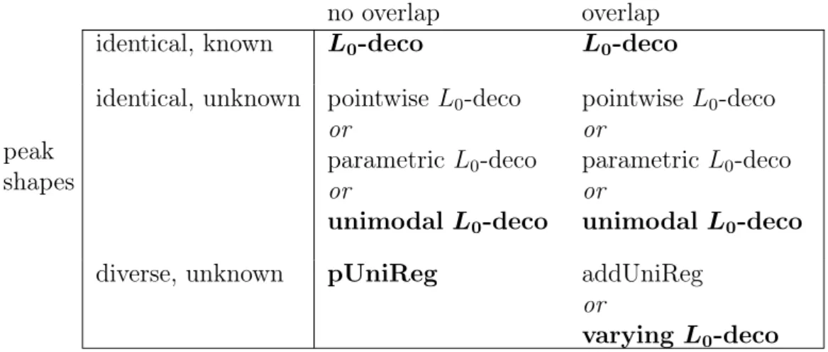
4.3.6 Applicability of the model types . . . . 54
5 Implementation 56 5.1 The R package uniReg . . . . 56
5.2 Bayesian unimodal spline regression . . . . 64
5.3 Multimodal regression . . . . 70
5.3.1 Deconvolution with a parametric peak shape . . . . 71
5.3.2 Deconvolution with a unimodal peak shape . . . . 74
5.3.3 Deconvolution with additive unimodal regression . . . . 77
5.3.4 Deconvolution with diverse unimodal peak shapes . . . . 79
6 Simulation study for unimodal regression 83 6.1 Data generation process . . . . 83
6.2 Compared methods and fitting process . . . . 85
6.3 Evaluation methods . . . . 88
6.4 Results . . . . 90
7 Applications 93 7.1 Unimodality: growth hormone dose-response analysis . . . . 93
7.2 Multimodality . . . . 96
7.2.1 Analysis of dive phases of marine animals . . . . 96
7.2.2 Astroparticle physics data analysis . . . . 99
7.2.3 Breath gas analysis with ion mobility spectrometry . . . 100
7.3 Further utilization of the proposed methodology . . . 105
7.3.1 Robust unimodal spline regression . . . 105
7.3.2 Mixture of constant and unimodal regression . . . 105
7.3.3 Additive unimodal regression as an intermediate step for classifi- cation of IMS data sets . . . 106
8 Summary and outlook 108
Bibliography 113
Appendix 121
A Additional tables 121
B Proofs 123
C The inverse Bayes formulae sampler for truncated multivariate normal ran-
dom sampling 128
D Documentations of auxiliary R functions 131
E Projecting vectors into the space of unimodal vectors with fixed mode 151
List of Figures
1.1 Dive of a marine animal with spline basis and fitted spline . . . . 3
2.1 Scatterplots of PST dosage vs. means of the response variables . . . . 7
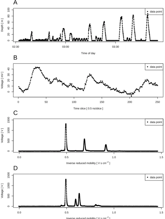
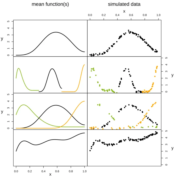
2.2 Multimodal example data sets used throughout the thesis. . . . 10
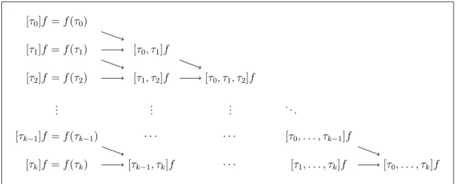
3.1 Triangular scheme for the calculation of divided differences . . . . 18
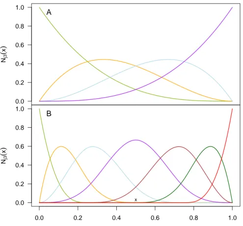
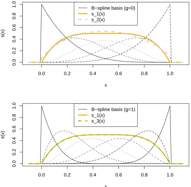
3.2 Comparison of Bernstein and B-spline basis . . . . 21
3.3 Example of a unimodal spline function with non-unimodal coefficients . . 31
4.1 Simulated examples . . . . 43
6.1 The nine function profiles used in the simulation study . . . . 84
6.2 Simulation results . . . . 92
7.1 Dose-response data with fitted spline functions . . . . 95
7.2 Spline regression for the diving depth example . . . . 98
7.3 FACT time series and fitted deconvolution model . . . 100
7.4 IMS spectra A and B with fitted piecewise unimodal regressions . . . 102
7.5 IMS spectrum A and L
0-deconvolution model with different peak shapes 103
7.6 IMS spectrum B and L
0-deconvolution model with different peak shapes 104
Notations
1 : indicator function, i.e., 1
A(x) =
1, x ∈ A 0, x / ∈ A 0
L: zero-vector of length L
1
L: one-vector of length L
I
L: identity matrix of dimension L × L
∆
q: differencing operator of order q V: Bernstein-Schoenberg operator η
k: space of spline functions of degree k
C
q: space of q-times continuously differentiable functions
P
k: space of polynomial functions of degree smaller or equal to k [a, b]
n: n-fold Cartesian product of the interval [a, b]
|M|: Cardinality of the set M
N
M(µ, Σ): Multivariate normal distribution with mean µ and covariance matrix Σ truncated to the set M ⊂ R
dIn general, lower-case letters (e.g., y) represent real numbers, that is, constants, obser- vations or indices, while their bold counterparts (e.g., y) stand for vectors and bold capital letters (e.g., Y ) for matrices of such numbers. Random variables are indicated by capital letters (e.g., Y ) and random vectors by bold, calligraphic letters (e.g., Y).
When taking the Bayesian perspective, especially, when parameters or parameter vectors
are considered random, we will not distinguish between the observation and its random
counterpart for convenience. In addition, a simplified notation for probability densities, which is commonly used in Bayesian statistics, will be employed. For example, the nota- tion p(β|y) stands for the conditional density p(β = β|Y = y), where β is the random counterpart of β.
Abbreviations
ADF Average daily feed consumption ADG Average daily gain of weight AIC Akaike information criterion ASE Average squared error
BIC Bayesian information criterion B-S Bernstein-Schoenberg
ed Effective Dimension
FACT First G-APD Cherenkov telescope G-APD Geiger-mode avalanche photodiods G/F Gain-to-feed ratio
IMS Ion mobility spectrometry
IRLS Iteratively re-weighted least squares MCC Multi capillary columns
MCMC Markov Chain Monte Carlo MCR Multivariate curve resolution MRL Mean relative loss
PST Porcine somatotropine
REML Restricted maximum likelihood
RSS Residual sum of squares
sigE Sigmoid E
maxTDR Time-depth-recorder
TPF Truncated power function
1 Introduction
1.1 Motivation
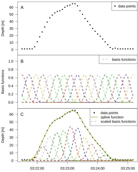
In statistical modelling, many approaches aim at describing the way in which some aspect in life changes depending on one or more variables in its environment. For example, the diving depth of a marine animal during a dive is first monotone increasing and then monotone decreasing over time, see Figure 1.1A. In explicit, there is a unimodal dependence on time.
Establishing a relationship between a dependent variable (response) and one or several independent variables (predictors) is called regression analysis. Usually, these variables are observed on the units of a certain population and the interest is in the mean of the response Y given the values x of the predictors X . In regression analysis the mean is modelled by a function f of the predictor values:
E(Y |X = x) = f(x),
where f is usually depending on a vector θ of parameters, f (x) = f (x|θ), to be esti- mated.
How many and which predictors to choose for a multiple regression model, is studied under the subject of variable selection. In this thesis however, the focus is on univariate regression.
For chosen variables X and Y there are, of course, still infinitely many possibilities to
specify f: first of all, one can assume a simple linear relationship as well as polynomial
functions, both of which can be estimated from data using linear model theory. If the
function is non-linear in the parameters, non-linear optimization algorithms can be used
to estimate θ (see, e.g., the book by Seber and Wild, 2003, on non-linear regression
techniques). In these cases, there are usually few parameters, since the gain from using
higher polynomial degrees is small and non-linear models with many parameters are
computationally hard to estimate. To sum up, parametric approaches are quite restric-
tive regarding the shapes of the function f that can be modelled. In other words, they pose so many assumptions about the underlying relationship that, if the true relationship deviates from them, a lot of bias is introduced. On the other hand, if the assumptions are justified, the variance of the estimated relationship between different samples is quite low. In pharmaceutical dose-response trials, for example, the functional form f used for the analysis has to be pre-specified in the study protocol (before data collection). This is very difficult and practical methods often rely on specification of a candidate set of parametric dose-response models (see, e.g., Bretz et al., 2005) and on model selection or model averaging.
Competitors to these procedures are regression approaches which do not specify the func- tional form of f by a set of parameters and are hence called non-parametric. They often rely on local estimation approaches, where no closed-form representation of f exists, for example, kernel smoothers such as nearest neighbour estimators or local polynomial re- gression (see, e.g., Chapter 6 of Hastie et al., 2009, for an introduction). These methods are – contradictory to the term "non-parametric" – also said to have infinitely many parameters. They are very flexible and usually have a low estimation bias, but the estimated relationships may vary strongly between different samples. Additionally, the estimated functions f are not necessarily differentiable or even discontinuous.
Semi-parametric approaches can be thought of as a compromise and are often charac- terized by many parameters. In addition, they usually describe the form of f as a linear combination of basis functions, for example, radial or B-spline basis functions (see also Figure 1.1B and C for an illustration of the latter). The coefficients of the linear com- bination are the parameters to be estimated.
The B-spline basis induces the popular class of polynomial spline functions, which are smooth piecewise polynomials. Using a large basis (many parameters) yields very flexible functions, which are continuous and differentiable up to a known degree. The function itself and its derivatives have a closed-form representation. Nevertheless, f can be esti- mated in terms of a linear model due to the linear combination of basis functions. Again, the flexibility reduces bias, but comes at the price of higher variability across samples from the same population.
The task of reducing the variance of the estimators without increasing the estimation bias has been tackled in two popular ways:
1. introduction of a smoothness penalty, dating back to the smoothing spline ap-
proaches by Reinsch (1967, 1971),
● ● ● ● ●
●
●
●
●
●
●
●
●
●
● ● ●
●
● ●
● ●
●
●
●
●
●
●
●
●
●
●
●
●
●
●
● ● ● ● ● ● ● ● ●
0 10 20 30 40 50 60
Depth [m]
●
data points
A
0.0 0.2 0.4 0.6 0.8 1.0
Basis functions
basis functions
B
● ● ● ● ●
●
●
●
●
●
●
●
●
●
● ●
●
●
● ●
● ●
●
●
●
●
●
●
●
●
●
●
●
●
●
●
● ● ● ● ● ● ● ● ●
03:22:00 03:23:00 03:24:00 03:25:00
0 10 20 30 40 50 60
Depth [m]
●
data points spline function
scaled basis functions
C
Figure 1.1: Dive of a marine animal with spline basis and fitted spline.
(A) Scatterplot of the diving depth [in m] of a marine animal versus time
(between 03:21:30 a.m. and 03:25:10 a.m. on January 6th 2002). It is an
excerpt from the data set divesTDR from R package diveMove (version 1.4.1,
cf. Luque, 2007). (B) B-spline basis functions. (C) Data from (A) and a fitted
spline function, which is the sum of the corresponding scaled B-spline basis
functions. In explicit, the spline is a linear combination of the B-spline basis
functions.
2. introduction of a shape constraint, dating back to constrained estimation ap- proaches from the 1950s (Brunk, 1955; Hildreth, 1954) and to the "pool adjacent violators algorithm" by Barlow et al. (1972) for pointwise monotone regression.
The first approach penalizes functions that are too variable and aims at finding a com- promise between over- and underfitting, between small bias and small variance. The second approach reduces the function space from which f is taken, which also decreases the variability. Shape constraints such as monotonicity or unimodality do not restrict the function space as severely as polynomial or non-linear parametric models and, therefore, the chance of violated assumptions and thus increased bias is smaller in those situa- tions. In addition, there are many applications in which the assumption of a certain shape constraint, such as positivity, monotonicity or unimodality, is very plausible and the incorporation of this prior knowledge into the model can only be advantageous. Re- garding the diving depth of a marine animal, for example, the assumption of a unimodal shape with respect to time seems likely, while something like a quadratic relationship is less easily justified.
1.2 Aims and outline
This thesis will consider the use of smoothness penalties and shape constraints as well as their combination in univariate regression. The focus will be on the shape constraint of unimodality, which has received less attention in the literature so far.
Unimodal regression – as a type of non-parametric shape-constrained regression – is a suitable choice in regression problems when the prior information about the underlying relationship between predictor and response is vague, but when it is (almost) certain that the response variable first increases with higher values of the predictor variable up to a maximum (or mode) and then decreases again.
While there exist a variety of parametric approaches to estimate a unimodal relation- ship, this thesis introduces a flexible semi-parametric method for estimating a smooth unimodal function based on spline functions. For this purpose, spline functions will be shown to be particularly well-suited for shape-constrained function estimation.
A prominent application, which will serve as an example several times during this the- sis, is dose-response analysis. Here, the (beneficial) effect of a substance increases with increasing dose up to a saturation point, after which the effect starts to decrease again, as the substance might cause, for example, interfering toxic effects.
However, the prior knowledge in different applications has various degrees of complexity
since data shapes may vary from (piecewise) unimodal relationships to accumulations of identically or even diversely shaped unimodal functions. This thesis argues that uni- modal regression is also useful in situations where the relationship between two variables is not unimodal, but multimodal, in explicit, the function f has several modes (local maxima). Therefore, this thesis also goes beyond unimodal regression and proposes to model multimodality using several unimodal functions.
The outline of this thesis is as follows: In Chapter 2 data sets from different areas are introduced to further motivate the need for unimodal regression and its multimodal extensions in real applications.The examples stem from dose-response analysis, marine biology, astroparticle physics and breath gas analysis.
Chapter 3 introduces regression splines and their smoothness-penalized pendants and highlights the benefits for regression purposes, especially in the presence of a shape con- straint such as unimodality. A frequentist as well as a Bayesian approach to unimodal spline regression are developed. The aim of Chapter 4 is to present methodology, which enables the handling of a broad spectrum of applications with multimodal data. Thus, several approaches, extending the methodology of Chapter 3, are proposed and recom- mendations on the method of choice in different situations are given. Both Chapters 3 and 4 provide a literature overview within the respective branch of research.
Chapter 5 introduces an R package which implements the frequentist unimodal regres- sion approach, and also describes implementational details of the other methods for unimodal and multimodal regression.
The performance of the proposed unimodal spline regression approaches in comparison to competing methods is assessed in Chapter 6 with an extensive simulation study in the dose-response analysis context. The question, if a combination of shape constraint and penalization is beneficial or if one of them suffices, is addressed there, too.
The usefulness of the methods in practice is demonstrated in Chapter 7 by applying the methodology to the real data examples from Chapter 2. The applications are increasing in complexity as they vary from unimodal or piecewise unimodal relationships to con- volutions of identically or even diversely shaped unimodal functions.
Chapter 8 summarises the thesis and provides an outlook on further extensibility of the
presented methodology and future research objectives.
material
This chapter describes application areas where unimodal regression can be useful and provides details on the respective data sets that are analysed throughout this thesis.
The fields of application are very diverse as the data sets stem from dose-response trials, marine biology, astroparticle physics and breath gas analysis.
2.1 Growth hormone dose response data
The first field of application is dose-response analysis, which was also discussed in Köll- mann et al. (2014).
Characterization of the dose-response relationship for desirable and undesirable effects of a pharmaceutical compound is the central problem of its clinical development. The pre-specification of one dose-response model for analysis in the study protocol (before data collection) is difficult, which is why practical methods often rely on specification of a candidate set of parametric dose-response models (see, e.g., Bretz et al., 2005) and on model selection or model averaging. Unimodal regression is a non-parametric competitor to these techniques.
A typical assumption in parametric as well as non-parametric dose-response analyses is monotonicity. However, in a variety of cases this assumption can be challenged as the interference of potential saturation or toxicity effects cannot be excluded. When considering a clinical utility index that combines efficacy and safety measures (see e.g.
Khan et al., 2009) one explicitly expects a unimodal relationship and a monotonically in- creasing curve would be surprising to observe. But even when considering efficacy alone unimodality can occur as in the example to follow. A unimodal shape constraint relaxes the assumption of monotonicity and is adequate whenever an umbrella dose-response curve cannot be excluded a priori.
The example data set originates from animal science, where the growth of pigs is eval-
●
●
● ● ●
0.7 0.8 0.9 1.0
PST dosage [mg/pig/day]
ADG [kg/day]
●
●
● ● ●
0.0 1.5 3.0 6.0 9.0
●
●
● ●
●
160 165 170 175 180 185 190
PST dosage [mg/pig/day]
Age [days]
●
●
● ●
●
0.0 1.5 3.0 6.0 9.0
●
●
●
●
●
0.25 0.30 0.35 0.40
PST dosage [mg/pig/day]
G/F
●
●
●
●
●
0.0 1.5 3.0 6.0 9.0
●
●
●
●
●
2.0 2.2 2.4 2.6 2.8 3.0
PST dosage [mg/pig/day]
ADF [kg/pig/day]
●
●
●
●
●
0.0 1.5 3.0 6.0 9.0
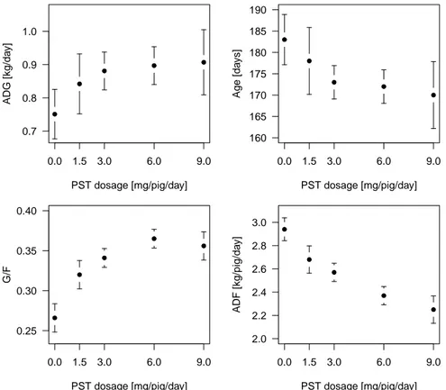
Figure 2.1: Scatterplots of PST dosage vs. means of the response variables.
The standard errors at each dose are indicated with bars. Data source:
McLaren et al. (1990).
uated in dependence of an increasing dose of a growth hormone. McLaren et al. (1990) investigated the relationship between administration of porcine somatotropin and several growth variables in 195 pigs. Details on the experimental procedure and data prepro- cessing can be found in their article. The (aggregated) data used here are the porcine somatotropin dosage levels [mg/pig/day] (PST) and the least squares means and stan- dard deviations of four response variables: Average daily gain of weight [kg/day] (ADG), age at 103.5 kg [days] (Age), gain-to-feed ratio (G/F) and average daily feed consump- tion [kg/pig/day] (ADF). The five dosage levels are 0, 1.5, 3, 6, 9 mg/pig/day and the means and standard errors at the respective levels correspond to 29, 29, 57, 58, and 22 pigs. The data are plotted in Figure 2.1 and the actual data values can be found in Table 2.1.
While the modes of the means of ADG, Age and ADF are at extreme doses (suggesting monotone relationships), the means of G/F have their mode in the interior at dose 6.
Since monotonicity is a special case of unimodality, it seems reasonable to relax the
monotonicity assumption and apply unimodal regression to all four variables (inverse unimodal for the variables Age and ADF). The results are presented in Section 7.1.
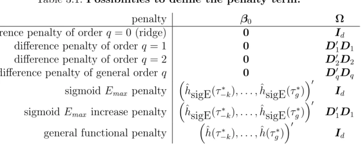
Table 2.1: Porcine somatotropin (PST) dosages [mg/pig/day] and least squares means and standard errors of the four performance vari- ables. ADG = average daily gain of weight [kg/d], Age = age at 103.5 kg [d], G/F = gain-to-feed ratio, ADF = average daily feed consumption [kg/pig/d].
Data source: McLaren et al. (1990).
PST dosage
0 1.5 3 6 9
ADG 0.751 (0.038) 0.842 (0.046) 0.881 (0.029) 0.897 (0.029) 0.907 (0.050)
Age 183 (3) 178 (4) 173 (2) 172 (2) 170 (4)
G/F 0.266 (0.009) 0.320 (0.009) 0.341 (0.006) 0.365 (0.006) 0.356 (0.009) ADF 2.940 (0.050) 2.680 (0.060) 2.570 (0.040) 2.370 (0.040) 2.250 (0.060)
2.2 Analysis of dive phases of marine animals
The second application example is the analysis of diving behaviour of marine animals (see also Köllmann et al., 2016). Time-depth-recorders (TDRs) measure the diving depth of marine animals such as seals or whales. The resulting data sets may contain measurements over several days at regular sampling frequencies. In the case of marine mammals, the animals repeatedly perform dives from the water surface down to various depths to find food and for other activities. An excerpt from such a TDR data set, taken from the R package diveMove (version 1.4.1, cf. Luque, 2007; Luque and Fried, 2011), is shown in Figure 2.2A.
Marine biologists are interested, among other things, in the detection of phases within a
dive which correspond to different behaviours (see e.g. Halsey et al., 2007). As claimed
by Halsey et al. (2007) there is need for objective and automated categorisation of the
diving behaviour and they develop a Matlab program that classifies diving depth data
using a set of pre-specified criteria. This approach does not consider measurement error,
which can be accounted for by modelling the dives statistically. This is, for example,
realized in version 1.4.1 of the R package diveMove by fitting multiple smoothing splines
to the data. Afterwards, the derivative of the fitted splines is used to divide the dives into
different phases like descent and ascent. In Section 7.2.1 we show that using piecewise
unimodal regression splines is advantageous for this purpose. Since the animal definitely needs to come back to the surface to draw breath, in explicit, since the dives do not overlap, the time series can be modelled by piecewise unimodality.
2.3 Astroparticle physics data analysis
The third field of application is astroparticle physics, which was also presented in Köll- mann et al. (2016). The First G-APD Cherenkov Telescope (FACT; see Anderhub et al., 2013; Biland et al., 2014) is used by astroparticle physicists to detect cosmic rays. These cosmic rays induce light flashes in the earth’s atmosphere, which can be used to calculate the primary particle’s properties. The camera of the telescope has several pixels and each pixel collects a signal, that is, a time series of measured voltages. See Figure 2.2B for an example with 250 observations.
Each photon hitting a camera pixel causes a change in the signal, which can be described by a unimodal loading curve with an amplitude of approximately 10 mV (Anderhub et al., 2013). The aim is to detect the arrival times and numbers of photons to draw conclu- sions about the type of the triggering particle (gamma or hadron). A good overall fit is of interest, too, since the integral over the signal is used in subsequent analyses. The shape of the signal is similar to that of a loading and unloading condenser and thus, physicists have suggested a parametric wave form for the change in the voltage due to the arrival of one or more photons. When n
pphotons arrive at time t
0this wave form is given by
U(t) = γ + n
p· U
0· 1 − e
−t−t0 ξ1
e
−t−t0
ξ2
![Table 2.1: Porcine somatotropin (PST) dosages [mg/pig/day] and least squares means and standard errors of the four performance vari-ables](https://thumb-eu.123doks.com/thumbv2/1library_info/3649105.1503193/18.892.121.769.331.464/table-porcine-somatotropin-dosages-squares-standard-errors-performance.webp)