Research Collection

(1)

Research Collection

Dataset

Integration of real-time traffic management and train control for rail networks

Supplementary material

Author(s):

Corman, Francesco Publication Date:

2018

Permanent Link:

https://doi.org/10.3929/ethz-b-000256447

Rights / License:

In Copyright - Non-Commercial Use Permitted

This page was generated automatically upon download from the ETH Zurich Research Collection. For more information please consult the Terms of use.

ETH Library

(2)

Appendix C Detailed experimental results for Part 2

Table 1 provides the objective values of the P

NLP

problem and the P

TSPO

problem, in the case of using the weighted-sum formulation.

Table 1. Objective value of the P

NLP

problem and the P

TSPO

problem with the weighted-sum formulation, corresponding to Fig. 2

Weights [delay, energy]

Objective value of the P_NLPproblem considering different computation time limits

Objective value of the P_TSPOproblem considering different computation time limits

Improvement in objective value (unit: %) 180 seconds 3600 seconds initial solution 180 seconds 3600 seconds 180 seconds 3600 seconds

[1,1] 89.75 89.68 84.72 79.51 77.70 11.41 13.36

[2,1] 94.12 93.75 89.63 88.05 85.16 6.45 9.17

[10,1] 132.47 132.72 128.85 125.31 126.37 5.40 4.79

[20,1] 184.43 184.38 177.87 174.02 172.82 5.64 6.27

[50,1] 344.62 343.94 324.96 318.67 317.47 7.53 7.70

[100,1] 611.63 606.10 570.06 559.52 554.79 8.52 8.47

[120,1] 723.09 710.08 668.12 655.51 646.98 9.35 8.89

[200,1] 1142.58 1111.18 1060.31 1035.79 1027.54 9.35 7.53

[500,1] 2535.81 2430.29 2531.04 2477.81 2452.05 2.29 -0.90

[1000,1] 4874.70 4749.70 4982.22 4875.38 4824.12 -0.01 -1.57

Table 2 presents the objective values of the two problems, in the case of using the ε-constraint formulation.

Table 2. Objective value (i.e., energy consumption) of the P

NLP

problem and the P

TSPO

problem with the ε-constraint formulation, corresponding to Fig. 3

Initial delays

Objective value of the PNLPproblem (unit: 10⁸J), considering different computation time limits

Objective value of the PTSPOproblem (unit: 10⁸J), considering different computation time limits

Improvement in objective value (unit: %) 180 seconds 600 seconds initial solution 180 seconds 300 seconds 600 seconds 180 seconds 600 seconds

I^delay_initial 80.08 79.34 79.82 76.74 76.14 75.49 4.16 4.04

I180s^delay 91.70 88.85 92.18 89.60 89.28 89.19 2.29 -0.49

I_300s^delay 95.14 93.60 96.59 93.81 93.79 93.77 1.40 -0.20

I_300s^delay 96.41 95.08 97.53 95.04 94.78 94.73 1.42 0.32

I3600s^delay 99.34 98.78 99.60 97.60 96.65 96.65 1.76 2.16

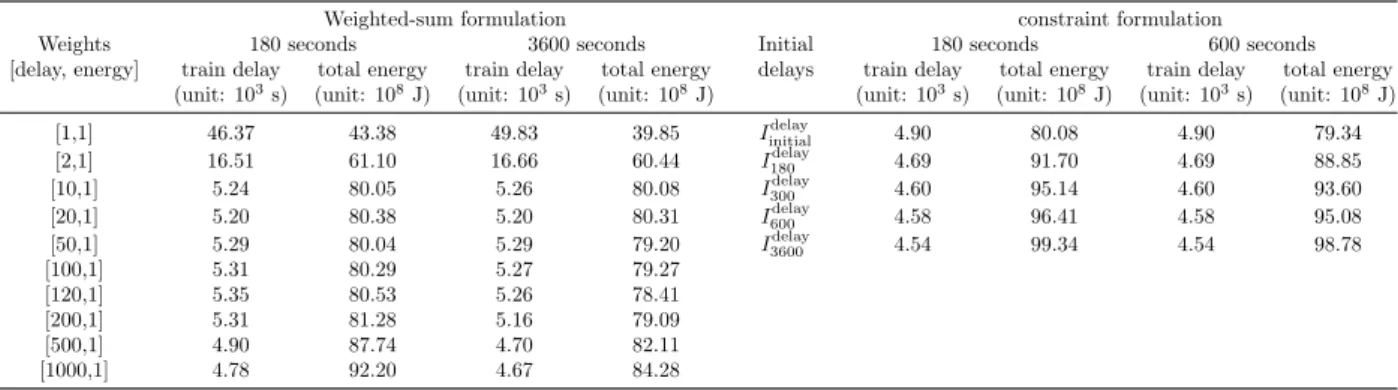
Table 3 provides the detailed results of the P

NLP

problem by using the weighted-sum formulation and the ε-constraint formulation respectively, in terms of train delay time and energy consumption. The unit of computation time and computation time limit is second, the unit of train delay time is 10

³

second, and the unit of energy consumption is 10

⁸

J. Table 3. Detailed results of the P

NLP

problem, in terms of train delay time and energy consumption

Weights [delay, energy]

Weighted-sum formulation

Initial delays

constraint formulation

180 seconds 3600 seconds 180 seconds 600 seconds

train delay (unit: 10

³

s)

total energy (unit: 10

⁸

J)

train delay (unit: 10

³

s)

total energy (unit: 10

⁸

J)

train delay (unit: 10

³

s)

total energy (unit: 10

⁸

J)

train delay (unit: 10

³

s)

total energy (unit: 10

⁸

J)

[1,1] 46.37 43.38 49.83 39.85

I_initial^delay

4.90 80.08 4.90 79.34

[2,1] 16.51 61.10 16.66 60.44

I₁₈₀^delay

4.69 91.70 4.69 88.85

[10,1] 5.24 80.05 5.26 80.08

I₃₀₀^delay

4.60 95.14 4.60 93.60

[20,1] 5.20 80.38 5.20 80.31

I₆₀₀^delay

4.58 96.41 4.58 95.08

[50,1] 5.29 80.04 5.29 79.20

I₃₆₀₀^delay

4.54 99.34 4.54 98.78

[100,1] 5.31 80.29 5.27 79.27

[120,1] 5.35 80.53 5.26 78.41

[200,1] 5.31 81.28 5.16 79.09

[500,1] 4.90 87.74 4.70 82.11

[1000,1] 4.78 92.20 4.67 84.28

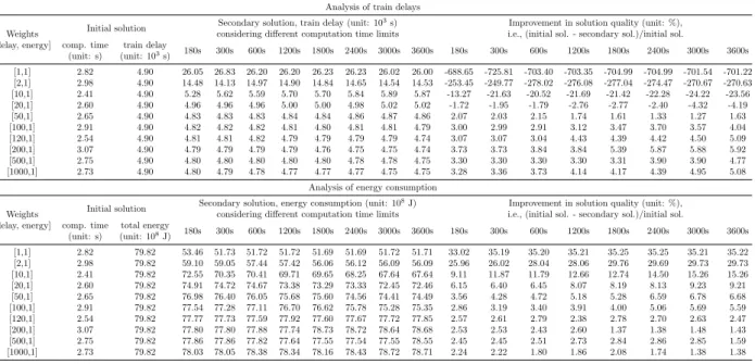
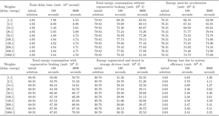
Tables 4 - 5 provide the detailed results of the P

TSPO

problem, considering the weighted-sum formulation and the ε-constraint formulation respectively, in terms of train delay time and energy consumption, as discussed in Section 4.2.

1

(3)

Table 4. Results of the P

_TSPO

problem, minimizing both train delay and energy consumption in the objective function, corresponding to Fig. 4

Analysis of train delays

Initial solution Secondary solution, train delay (unit: 10³s) considering different computation time limits

Improvement in solution quality (unit: %), i.e., (initial sol. - secondary sol.)/initial sol.

comp. time (unit: s)

train delay

(unit: 10³s) 180s 300s 600s 1200s 1800s 2400s 3000s 3600s 180s 300s 600s 1200s 1800s 2400s 3000s 3600s [1,1] 2.82 4.90 26.05 26.83 26.20 26.20 26.23 26.23 26.02 26.00 -688.65 -725.81 -703.40 -703.35 -704.99 -704.99 -701.54 -701.22 [2,1] 2.98 4.90 14.48 14.13 14.97 14.90 14.84 14.65 14.54 14.53 -253.45 -249.77 -278.02 -276.08 -277.04 -274.47 -270.67 -270.63

[10,1] 2.41 4.90 5.28 5.62 5.59 5.70 5.70 5.84 5.89 5.87 -13.27 -21.63 -20.52 -21.69 -21.42 -22.28 -24.22 -23.56

[20,1] 2.60 4.90 4.96 4.96 4.96 5.00 5.00 4.98 5.02 5.02 -1.72 -1.95 -1.79 -2.76 -2.77 -2.40 -4.32 -4.19

[50,1] 2.65 4.90 4.83 4.83 4.83 4.84 4.84 4.86 4.87 4.86 2.07 2.03 2.15 1.74 1.61 1.33 1.27 1.63

[100,1] 2.91 4.90 4.82 4.82 4.82 4.81 4.80 4.81 4.81 4.79 3.00 2.99 2.91 3.12 3.47 3.70 3.57 4.04

[120,1] 2.54 4.90 4.81 4.81 4.82 4.79 4.79 4.79 4.79 4.74 3.07 3.07 3.04 4.43 4.39 4.42 4.50 5.09

[200,1] 3.07 4.90 4.79 4.79 4.79 4.79 4.76 4.75 4.75 4.74 3.73 3.73 3.84 3.84 5.39 5.87 5.88 5.92

[500,1] 2.75 4.90 4.80 4.80 4.80 4.80 4.80 4.78 4.78 4.75 3.30 3.30 3.30 3.30 3.31 3.90 3.90 4.77

[1000,1] 2.73 4.90 4.80 4.79 4.78 4.77 4.77 4.77 4.75 4.75 3.28 3.36 3.73 4.14 4.17 4.39 4.95 5.08

Analysis of energy consumption

Initial solution Secondary solution, energy consumption (unit: 10⁸J) considering different computation time limits

total energy

(unit: 10⁸J) 180s 300s 600s 1200s 1800s 2400s 3000s 3600s 180s 300s 600s 1200s 1800s 2400s 3000s 3600s

[1,1] 2.82 79.82 53.46 51.73 51.72 51.72 51.69 51.69 51.72 51.71 33.02 35.19 35.20 35.21 35.25 35.25 35.21 35.22

[2,1] 2.98 79.82 59.10 59.05 57.44 57.42 56.06 56.12 56.09 56.09 25.96 26.02 28.04 28.06 29.76 29.69 29.73 29.73

[10,1] 2.41 79.82 72.55 70.35 70.41 69.71 69.65 68.25 67.64 67.64 9.11 11.87 11.79 12.66 12.74 14.50 15.26 15.26

[20,1] 2.60 79.82 74.91 74.72 74.67 73.38 73.29 73.33 72.45 72.46 6.15 6.40 6.45 8.07 8.19 8.13 9.23 9.21

[50,1] 2.65 79.82 76.98 76.40 76.05 75.68 75.60 74.56 74.41 74.49 3.56 4.28 4.72 5.18 5.28 6.59 6.78 6.68

[100,1] 2.91 79.82 77.54 77.28 77.11 76.70 76.62 75.78 75.28 75.35 2.86 3.19 3.40 3.91 4.00 5.06 5.69 5.59

[120,1] 2.54 79.82 77.77 77.73 77.59 77.92 77.60 77.67 77.72 77.85 2.57 2.61 2.79 2.38 2.78 2.70 2.63 2.47

[200,1] 3.07 79.82 77.80 77.80 77.88 77.74 78.73 78.72 78.64 78.68 2.53 2.53 2.43 2.60 1.37 1.38 1.48 1.43

[500,1] 2.75 79.82 77.86 77.86 77.82 77.64 77.55 77.54 77.55 78.55 2.45 2.45 2.51 2.73 2.84 2.86 2.85 1.59

[1000,1] 2.73 79.82 78.03 78.05 78.38 78.34 78.16 78.43 78.72 78.71 2.24 2.22 1.80 1.86 2.08 1.74 1.38 1.38

Table 5. Results of the P

TSPO

problem, minimizing energy consumption in the objective function with respect to an upper bound for the train delay, corresponding to the analysis of Fig. 5

Analysis of the train delays

Initial delays

Initial solution Secondary solution, train delay (unit: 10³s) considering different computation time limits

train delay

(unit: 10³s) 180 seconds 300 seconds 600 seconds 180 seconds 300 seconds 600 seconds

I_initial^delay 0.90 4.90 4.90 4.90 4.90 0.00 0.00 0.00

I_180s^delay 0.85 4.69 4.69 4.69 4.69 0.00 0.00 0.00

I300s^delay 0.81 4.60 4.60 4.60 4.60 0.00 0.00 0.00

I600s^delay 0.80 4.58 4.58 4.58 4.58 0.00 0.00 0.00

I^delay_3600s 0.82 4.54 4.54 4.54 4.54 0.00 0.00 0.00

Analysis of the total energy consumption

Initial delays

Initial solution Secondary solution, energy consumption (unit: 10⁸J) considering different computation time limits

total energy

(unit: 10⁸J) 180 seconds 300 seconds 600 seconds 180 seconds 300 seconds 600 seconds

I_initial^delay 0.90 79.82 76.74 76.14 75.49 3.85 4.61 5.43

I_180s^delay 0.85 92.18 89.60 89.28 89.19 2.72 3.08 3.20

I300s^delay 0.81 96.59 93.81 93.79 93.77 2.47 2.75 2.80

I600s^delay 0.80 97.53 95.04 94.78 94.73 2.86 2.86 2.88

I^delay_3600s 0.82 99.60 97.60 96.65 96.65 2.00 2.99 2.99

2

(4)

Table 6 presents the results of applying regenerative braking, in terms of train delay and energy con- sumption. These results are obtained by using the P

_TSPO

approach with the weighted-sum formulation.

Table 6. Results of the P

TSPO

approach with the weighted-sum formulation, when applying regenerative braking, corresponding to Fig. 6 and Fig. 7

Weights [delay, energy]

Train delay time (unit: 10

³

second) Total energy consumption without regenerative braking (unit: 10

⁸

J)

Energy used for acceleration (unit: 10

⁸

J) initial

solution

180 seconds

3600 seconds

initial solution

180 seconds

3600 seconds

initial solution

180 seconds

3600 seconds

[1,1] 4.94 7.98 8.53 79.82 69.38 65.84 76.31 66.10 62.69

[2,1] 4.93 6.69 6.98 79.82 70.69 69.13 76.31 67.34 65.85

[10,1] 4.93 5.40 5.61 79.82 72.30 68.87 76.31 68.92 65.65

[20,1] 4.93 5.05 5.00 79.82 75.24 74.26 76.31 71.77 70.84

[50,1] 4.93 4.89 4.73 79.82 76.93 77.26 76.31 73.45 73.78

[100,1] 4.93 4.84 4.74 79.82 77.73 78.15 76.31 74.24 74.66

[120,1] 4.93 4.82 4.74 79.82 78.86 77.43 76.31 75.35 73.96

[200,1] 4.93 4.84 4.71 79.82 78.42 77.83 76.31 74.92 74.34

[500,1] 4.93 4.84 4.71 79.82 77.95 77.89 76.31 74.46 74.90

[1000,1] 4.93 4.84 4.70 79.82 78.22 81.24 76.31 74.72 77.69

Weights [delay, energy]

Total energy consumption with regenerative braking (unit: 10

⁸

J)

Energy regenerated and stored in storage devices (unit: 10

⁸

J)

Energy loss due to system efficiency (unit: 10

⁸