Constraining parameters in marine pelagic ecosystem models – is it actually feasible with typical observations of standing stocks?

(1)

www.ocean-sci.net/11/573/2015/

doi:10.5194/os-11-573-2015

Constraining parameters in marine pelagic ecosystem models – is it actually feasible with typical observations of standing stocks?

U. Löptien and H. Dietze

GEOMAR Helmholtz Centre for Ocean Research Kiel, Düsternbrooker Weg 20, 24105 Kiel, Germany Correspondence to: U. Löptien (uloeptien@geomar.de)

Received: 5 December 2014 – Published in Ocean Sci. Discuss.: 12 February 2015 Revised: 25 June 2015 – Accepted: 28 June 2015 – Published: 20 July 2015

Abstract. In a changing climate, marine pelagic biogeo- chemistry may modulate the atmospheric concentrations of climate-relevant species such as CO₂ and N₂O. To date, projections rely on earth system models, featuring simple pelagic biogeochemical model components, embedded into 3-D ocean circulation models. Most of these biogeochemical model components rely on the hyperbolic Michaelis–Menten (MM) formulation which specifies the limiting effect of light and nutrients on carbon assimilation by autotrophic phytoplankton. The respective MM constants, along with other model parameters, of 3-D coupled biogeochemical ocean- circulation models are usually tuned; the parameters are changed until a “reasonable” similarity to observed standing stocks is achieved.

Here, we explore with twin experiments (or synthetic “observations”) the demands on observations that allow for a more objective estimation of model parameters. We start with parameter retrieval experiments based on “perfect” (synthetic) observations which we distort, step by step, by low- frequency noise to approach realistic conditions. Finally, we confirm our findings with real-world observations. In summary, we find that MM constants are especially hard to constrain because even modest noise (10 %) inherent to observations may hinder the parameter retrieval already. This is of concern since the MM parameters are key to the model’s sensitivity to anticipated changes in the external conditions. Fur- thermore, we illustrate problems caused by high-order parameter dependencies when parameter estimation is based on sparse observations of standing stocks. Somewhat counter to intuition, we find that more observational data can sometimes degrade the ability to constrain certain parameters.

1 Introduction

The challenges of a warming climate, and our apparent in- ability to significantly reduce emissions of climate-relevant species into the atmosphere, fuel a discussion on geoengi- neering options. Among the circulating ideas is ocean fertil- ization on a large scale. There, the underlying assumption is that the supply of nutrients to the sun-lit, nutrient-depleted surface ocean will increase biotic carbon sequestration away from the atmosphere (e.g. Williamson et al., 2012). However, because of the often non-linear and complex entanglements of relevant processes, an evaluation of such approaches is not straightforward. To this end, studies like Yool et al. (2009), Dutreuil et al. (2009), and Oschlies et al. (2010), which apply numerical earth system models comprising presumably most of the fundamental feed-back mechanisms, appear to be best suited to address pressing questions.

On the other hand, projections of earth system models are uncertain because the current generation of pelagic ecosystem models are, in contrast to the physical modules, based on empirical relationships, rather than being derived from first principles. The associated problem is two-fold.

First, there is no proof that the ubiquitous, so-called N–P–

Z–D (nutrient–phytoplankton–zooplankton–detritus) pelagic ecosystem models, which are at the core of most biogeochemical modules, are an admissible mathematical description of the real world (e.g. Anderson, 2005). This specifically applies to systems that are exposed to extreme conditions by a warming climate or large-scale ocean fertiliza- tion (e.g. Löptien, 2011). Second, biogeochemical models depend on many parameters, mostly describing rates (such as e.g. the maximum growth rate of phytoplankton), which are, even though they exert crucial control on the model behaviour (e.g. Kriest et al., 2010), per se, not known. The need

(2)

to address the latter issue is reflected in an increasing number of studies which aim to optimize the free model parameters mainly from observations of standing stocks, while few studies additionally include rate estimates (e.g. Fan and Lv, 2009; Friedrichs et al., 2006; Rückelt et al., 2010; Schar- tau, 2003; Spitz et al., 1998; Tjiputra et al., 2007; Hem- mings and Challenor, 2012; Matear, 1995; Ward et al., 2010;

Xiao and Friedrichs, 2014). Nevertheless, it is in practice often impossible to determine an optimal parameter set (Ward et al., 2010; Schartau et al., 2001; Rückelt et al., 2010). We can, admittedly, not rule out that the definition of the model–

data misfit (cost) is at the core of these problems and this has to be investigated in studies to come. Nevertheless, sat- isfactory results for cost functions other than the one applied in this study appear unlikely because the above mentioned studies comprise a wide range of cost functions already and, even so, report similar problems. Several conclusions were drawn from these parameter estimation attempts. For example, Matear (1995) concludes that the optimization problem might be underdetermined while Fasham et al. (1995) and Fennel et al. (2001) assume that the underlying equations do not represent actual processes and conditions.

Due to the manifold problems, it is common practice in the 3-D coupled ocean circulation ecosystem modelling commu- nity to assume that the model equations are accurate and to determine parameters which aim to achieve a “reasonable”

similarity to observations of standing stocks of prognostic variables. We mimic this approach focusing on the parameter uncertainty only, while we presume that the N–P–Z–D model equations are accurate.

Major problems associated with parameter selection in 3-D coupled ocean circulation biogeochemical models are caused by the sparseness of observations in space and time (e.g. Lawson et al., 1996). Also, biases and deficiencies in the physical models aggravate the comparison to real data (Friedrichs et al., 2006; Sinha et al., 2010; Dietze and Löp- tien, 2013). In addition, high computational costs hinder the search for the optimal parameter set because only a limited number of sets can be tested.

In this study we put the assumption to the test that parameter estimation relying on typical observations of standing stocks is feasible if enough computational resources were available. We use a simple modelling framework (box model) that is computationally cheap such that many thousands of parameter combinations can be tested. We conduct twin experiments (i.e. we construct our own genuine truth that is consistent with our model equations). By this approach, we can control the sparseness and noise levels of (synthetic) observations used to retrieve parameter sets with optimization techniques.

Foregoing similar approaches of Lawson et al. (1996), Schartau et al. (2001) and Spitz et al. (1998) indicate that it should be possible to recover most model parameters, when using various sampling strategies or when the synthetic observations are disrupted with white noise. Our study adds to

the discussion by using an even more idealized model setup, which makes the interpretation of the results easier and saves computational cost. Furthermore, we use reddish noise to disrupt the genuine truth, as reddish noise is more typical for oceanic conditions than the white noise considered in earlier studies (Hasselmann, 1976). Note that our definition of noise is ambiguous. Generally, noise is defined as a random, unbiased modification of the genuine truth, effected by e.g.

measurement inaccuracy. In parameter optimization based on real-world observations, however, the definition of noise is often broadened and refers to noise effected by the combined effects of all unresolved processes that can cause deviations between simulated and observed values. These unresolved processes comprise e.g. the effects of uncertainties in the external forcing or boundary conditions that drive the model as well as unresolved mesoscale processes in the ocean.

In the following section, we describe the design of the numerical experiments: Sects. 2.1, 2.2 and 2.3 present the model equations, the external forcing and the optimization techniques, respectively. Section 2.3 does also introduce our quantitative measure of model performance, the so-called

“cost function”. The underlying observations, the synthetic data sets from the twin experiments, and the real-world set are described in Sect. 2.4. Section 2.5 lists all numerical experiments. In Sects. 3 and 4 we present and discuss our results. Section 5 closes with a summary.

2 Methods 2.1 Model

We use an N–P–Z–D model similar to those used by Yool et al. (2009), Dutreuil et al. (2009), Oschlies et al. (2010), Oschlies and Garcon (1999), Oschlies (2002), and Franks (2002). Our configuration is simpler in that it comprises one grid box only. This box resembles the surface mixed layer at a given location. Our approach is computationally cheap and enables us to test many thousands of parameter combinations during the search for optimal parameter sets.

Our prognostic variables are, as indicated by the name N–P–Z–D, nitrate (N), phytoplankton (P), zooplankton (Z) and detritus (D). In a nutshell, phytoplankton takes up nitrate during growth fuelled by photosynthetically available radiation (PAR). If phytoplankton lacks nitrate or PAR, or both, its growth is hampered. Phytoplankton is grazed on by zooplankton. Both P and Z contribute to particulate organic matter, here called detritus (D). These contributions represent e.g. dead plankton and fecal pellets. D is reminer- alized back to nitrate which closes the cycle. An additional, faster loop from P and Z to N represents e.g. extracellular release and “messy feeding”. It might be noteworthy that reliable observations of D and Z are rare. Even so they are typically (as in our case) explicitly represented in order to simulate the effects of sinking organic matter and as a means

(3)

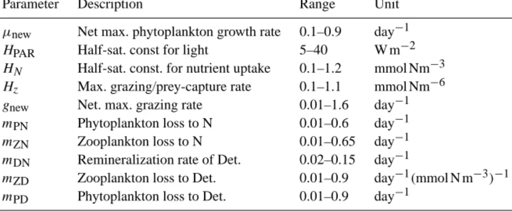
Table 1. Model parameters and associated ranges explored in this study.

Parameter Description Range Unit

µnew Net max. phytoplankton growth rate 0.1–0.9 day⁻¹

H_PAR Half-sat. const for light 5–40 W m⁻²

H_N Half-sat. const. for nutrient uptake 0.1–1.2 mmol Nm⁻³ H_z Max. grazing/prey-capture rate 0.1–1.1 mmol Nm⁻⁶

gnew Net. max. grazing rate 0.01–1.6 day⁻¹

m_PN Phytoplankton loss to N 0.01–0.6 day⁻¹

m_ZN Zooplankton loss to N 0.01–0.65 day⁻¹

m_DN Remineralization rate of Det. 0.02–0.15 day⁻¹

m_ZD Zooplankton loss to Det. 0.01–0.9 day⁻¹(mmol N m⁻³)⁻¹ m_PD Phytoplankton loss to Det. 0.01–0.9 day⁻¹

to mimic the (typically) rapid termination of phytoplankton spring blooms.

Our prognostic equations that determine the temporal evolution of nitrate (N), phytoplankton (P), zooplankton (Z) and detritus (D) are

d

dtN= −µmax·g_I·g_N·P+m_PN·P+m_ZN·Z+m_DN·D (1) d

dtP=µ_max·g_I·g_N·P−m_PN·P−G(P )·Z−m_PD·P (2) d

dtZ=G(P )·Z−mZN·Z−mZD·Z² (3) d

dtD=m_ZD·Z²+m_PD·P−m_DN·D. (4) All prognostic variables are scaled to units mmol Nm⁻³. gI= ^PAR

PAR+H_PAR and gN= ^N

N+H_N are the hyperbolic MM equations describing the limiting effect of light (here PAR refers to photosynthetically available radiation averaged over 24 h and the surface mixed layer) and of nitrate on nitrate uptake (Eq. 1) by phytoplankton (Eq. 2), respectively. The termsm_PN·P,m_ZN·Z andm_DN·D in Eq. (1) represent linear mortality of phytoplankton, zooplankton and remineralization of detritus, respectively. The zooplankton equation (Eq. 3) comprises two non-linear terms: first, the “Holling III-type” term

G(P)= g_maxP² P²+Hz

, (5)

with the maximum grazing rate, gmax, and the quotient of maximum grazing and prey-capture rate , Hz:=gmax/.

The second, non-linear term in the zooplankton equation (Eq. 3) is the quadratic mortalitym_ZD·Z².

The behaviour of the system of partial differential equations (1)–(4) is determined by parameters such as maximum growth rates (e.g.µ_maxin Eqs. 1 and 2) and the MM parameters (also referred to as half-saturation constants)H_PARand H_Nin Eqs. (1) and (2). These parameters are generally only poorly constrained and thus optimized.

Growth and loss of phytoplankton are antagonistically af- fecting phytoplankton stock. An infinite number of combinations of growth-related and loss-related parameters determines a system in which no phytoplankton will ever emerge.

These systems are not of interest here and in order to steer the parameter search away from the parameter space without any net phytoplankton growth, we define

µ_new:=µ_max−m_PN−m_PD. (6) By substitutingµmaxby µnew and by specifying µnew>0, we guide the optimization algorithm to search only among those parameter combinations which can yield net phytoplankton growth. Thus, definition (6) reduces the number of required model integrations considerably. In a similar man- ner we merge the maximum grazing rate (g_maxin Eq. 5) with the linear zooplankton mortality (m_ZNin Eqs. 1 and 3) such that

gnew:=gmax−mZN. (7)

These definitions do not reduce the number of free parameters (because the loss ratesm_PN, m_PDandm_ZNare still optimized), but makes the optimizations computationally more efficient. A side aspect is that obvious and strong dependency betweenµ_maxandm_PD(and betweeng_maxandm_ZN) is avoided.

The 10 free model parameters are listed in Table 1. To avoid unrealistic values, we restrict their allowed ranges (Ta- ble 1), following e.g. Schartau (2003). Note that in our ter- minology “model parameters” are constants and not to be confused with “prognostic variables” (N, P, Z and D).

2.2 Setup, external forcing and initialization

For the sake of simplicity and low computational cost, we consider a system that is homogenous in space, both in hori- zontal and in vertical direction. As a direct consequence, we do not have to account for advective and diffusive transport processes because their divergences, owed to the spacial ho- mogeneity, are always null. To this end we have a closed system – and a highly idealized one. This holds also because

(4)

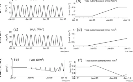
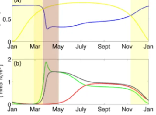
Figure 1. (a–b) Forcing OPTI: (a) shows the photosynthetically available radiation (PAR) averaged over 24 h and the surface mixed layer and (b) the total fixed nitrogen in the system. (c–d) like (a–b) but for SENSI, (e) PAR difference, SENSI – OPTI. (f) Difference in total nutrient content, SENSI – OPTI.

we do not resolve the process of detritus sinking out of the euphotic zone (which is an important process contributing to the “biological pump” of carbon in the ocean). However, this implication does not affect our rather generic conclusions which apply also, probably even more so, to models of a higher complexity (i.e. models that include more prognostic variables, or are coupled to a more complex physics).

We prescribe the photosynthetically available radiation (PAR) averaged over 24 h and the surface mixed layer. The seasonal variation affected by the combination of solar zenith angle, water turbidity (Löptien and Meier, 2011), cloudiness and surface mixed layer (Hordoir and Meier, 2012) depth is idealized by a sinusoid. Our PAR ranges from 2 W m⁻² in winter to 50 W m⁻² in summer. This range is representative of the surface mixed layer conditions in the Baltic Sea (Leppäranta and Myrberg, 2009). In addition to PAR, we prescribe the total amount of fixed nitrogen in the system. Our choice of 3 to 4.5 mmol Nm⁻³is typical for the sun-lit surface of the Baltic Sea (e.g. Neumann and Schernewski, 2008, their Fig. 10). The combination of prescribed PAR and the total amount of fixed nitrogen are subsequently referred to as the “forcing data set”.

We apply two forcing data sets in this study, which we name OPTI and SENSI. OPTI is applied whenever model parameters are optimized. We will find, in some cases, that very differing parameter sets yield almost identical, or at least very similar, solutions when driven by OPTI. In those cases we will test if the apparent similarity among the model simulations is preserved when the external forcing is slightly modified, i.e. when it is changed from OPTI to SENSI.

The rationale behind the design of OPTI and SENSI is – As idealized as possible, but yet, similar to real-world

conditions in the Baltic Sea.

– OPTI and SENSI should be as similar to one another as possible, and yet different enough to illustrate that parameter sets that feature similar solutions when driven by OPTI may well differ substantially when driven by SENSI.

Forcing data set OPTI is shown in Fig. 1: the PAR features a steady seasonal cycle until year 9, when the summer maximum decreases at a rate of 3.6 W m⁻²yr⁻¹. The nitrate inventory is set constant at 3.3 mmol Nm⁻³until year 5, increases at a rate of 0.2 mmol Nm⁻³yr⁻¹between year 5 and 11, and set constant at 4.5 mmol Nm⁻³thereafter. Both, this reduction of PAR and this increase of nutrients (each by≈30 %), are of a magnitude similar to changes detected during the previous decades in the Baltic Sea (Sanden and Håkansson, 1996; Kratzer et al., 2003; Sanden and Rahm, 1993). This does also apply to SENSI (Fig. 1b) which is, as discussed above, very similar to OPTI. The differences between OPTI and SENSI (Fig. 1e and f) are a slightly lower nitrate inventory with a weaker trend in SENSI, an earlier PAR decrease and a modified seasonal PAR-cycle, as depicted in Fig. 1c.

The initial values for phytoplankton, zooplankton, detritus and nitrate in OPTI are set to 0.1,0.1,0.1 and 3 mmol Nm⁻³, respectively. Note however that our simple model configuration is not sensitive to the initial distribution of total nitrogen among the prognostic variables. After 1 year, the model solutions are barely distinguishable from one another (this holds, of course, only if zooplankton and phytoplankton are initial- ized with values greater than zero). Hence we discard the first year of simulation in all model–data misfits presented here.

Thereafter the simulation is determined by the model parameters, the external forcing, and the initial total fixed nitrogen in the system – rather than being affected by the initial distribution of nitrogen among the prognostic variables.

(5)

2.3 Cost function and optimization

This study explores the requirements for an estimation of model parameters based on parameter optimization. A precondition for such an approach is the definition of a numerical measure of the misfit between the model simulations and data (i.e. synthetic or real-world observations). To define such a measure, or metric, is not straightforward and there are various approaches, including rather sophisticated ones based on correlations and Fourier transformations (e.g.

Stow et al., 2009). That said, we pragmatically chose the sum of the weighted squared differences between the model and data, for no other reasons than (1) this metric is commonly applied in the field of optimization of pelagic ecosystem models (e.g. Ward et al., 2010; Schartau et al., 2001;

Rückelt et al., 2010) and (2) systematic analyses of other cost functions are beyond the scope of this study. We define the cost functionJas

J = v u u t

1 M

M

X

m=1

W_m² 1 Nm

Nm

X

j=1

a_j− ˆa_j2

!

. (8)

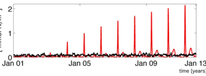
Mdenotes the number of prognostic variables,N_mthe number of data values (i.e. synthetic or real-world observations) of each prognostic variable,a_j a data value at timej andaˆ_j the corresponding model result.W_m determines the weight that each data–model pair contributes to the overall costJ. It is known that different weighting strategies can yield differing optimization results (e.g. Evans, 2003). The problem is that weighting (or no weighting) adds a subjective element to the optimization process. As we convert all prognostic variables to the same units (mmol Nm⁻³), we make a pragmatic choice and compute the costJ with equal weights,W_m=1 (in agreement with e.g. Prunet et al., 1996; Stow et al., 2009), which is usually referred to as root mean squared error (RMSE). IfN₁=N₂=N₃=N₄, this approach assumes implicitly that all state variables can be measured equally well at all time steps. Note that we consider some deviations from this assumption by investigating sparse data (which is equivalent to testing a different weighting), as described in Sect. 2.5. For the sparse data experiments, we calculate the RMSE based on only a part of the synthetic truth, assuming that the measurements are restricted to certain periods. All dataaj (synthetic and real-world observations) used in this study are converted to the same units (mmol Nm⁻³) and the noise added to disrupt the synthetic truth is of the same order of magnitude for all prognostic variables. In some cases (Figs. 3, 5 and 7) we will consider the time evolution of the model–data misfit, which is equivalent to omitting the time average in the definition of the cost function:

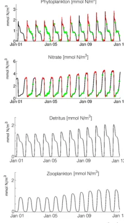
Figure 2. Subsampling of the genuine truth in SPARSE1 and SPARSE2. The black lines in the respective subpanels refer to the genuine truth simulation (based on the parameter set “truth” in Ta- ble 3 under forcing OPTI) of phytoplankton, nitrate, detritus and zooplankton. The green circles show SPARSE1 subsamples distorted by “level 1” noise (Sect. 2.5). The combination of red dots (also distorted by “level 1” noise) and green circles refers to data used in SPARSE2.

Jj = v u u t

1 M

M

X

m=1

W_m² aj− ˆaj2

!

. (9)

The cost is minimized by an automated numerical optimization, known as simulated annealing (Belisle, 1992), followed by a down-gradient search (Lagarias et al., 1998). We pro- vide a more detailed description in Appendix A. Note that the results of Ward et al. (2010) indicate that the choice of the optimization method is not so crucial if enough model integrations can be afforded (which is the case in our computationally cheap setups).

2.4 Data – synthetic and real-world observations We use two sorts of data, synthetic and real-world observations (cf. Table 2). The synthetic “observations” are constructed by subsampling a model simulation (Fig. 2). We apply a range of subsampling strategies as explained in the

(6)

Table 2. Parameter retrieval experiments. The experiments are based on different sets of observations (Sects. 2.4, 2.5) and aim to retrieve all, or a subset of the model parameters listed in Table 1 simultaneously.

Experiment Data Retrieved parameters

EASY Synthetic; daily sampling of all prognostic variables 10 NOISE Synthetic + (various) noise levels; daily sampling of all prog-

nostic variables (N, P, Z, D)

10 MISSING-ZD Synthetic + (various) noise levels; daily sampling of phyto-

plankton (P) and nitrate (N)

10 SPARSE1 Synthetic + level 1 noise; sparse and irregular sampling con-

fined to autumn of phytoplankton (P) and nitrate (N)

10 SPARSE2 Synthetic + level 1 noise; sparse and irregular sampling of phy-

toplankton (P) and nitrate (N) throughout the year but predomi- nated by late winter and spring samples; extension of SPARSE1

10

OBS10 Real-world observations of phytoplankton (P) and nitrate (N);

station BY5

10 OBS4 Real-world observations of phytoplankton (P) and nitrate (N);

station BY5

4 (µ_new,m_PD,m_DN,g_new)

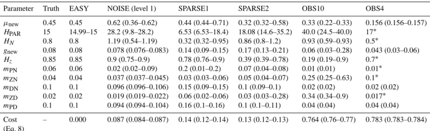
Table 3. Genuine truth parameter set (column 2) and estimates (column 3–8) obtained by the parameter retrieval experiments described in Table 2. The values in column 3 to 8 correspond to the first ensemble member of each retrieval experiment. In brackets we list the range enveloped by all ensemble members.

Parameter Truth EASY NOISE (level 1) SPARSE1 SPARSE2 OBS10 OBS4

µnew 0.45 0.45 0.62 (0.36–0.62) 0.44 (0.44–0.71) 0.32 (0.32–0.58) 0.33 (0.22–0.33) 0.156 (0.156–0.157) H_PAR 15 14.99–15 28.2 (9.8–28.2) 6.53 (6.53–18.4) 18.08 (14.6–35.2) 40.0 (24.5–40.0) 17^∗

HN 0.8 0.8 1.19 (0.54–1.19) 0.32 (0.32–0.95) 0.86 (0.8–1.2) 0.93 (0.59–0.93) 0.5^∗

gnew 0.08 0.08 0.078 (0.076–0.083) 0.14 (0.09–0.15) 0.17 (0.13–0.21) 0.06 (0.03–0.28) 0.043 (0.03–0.06) Hz 0.85 0.85 0.9 (0.75–0.9) 0.78 (0.76–0.9) 0.39 (0.39–0.78) 0.19 (0.19–0.9) 0.7^∗

m_PN 0.06 0.06 0.02 (0.02–0.09) 0.2 (0.01–0.2) 0.07 (0.04–0.08) 0.01 (0.01) 0.01^∗ mZN 0.04 0.04 0.037 (0.037–0.045) 0.03 (0.03–0.06) 0.05 (0.04–0.07) 0.25 (0.25–0.63) 0.1^∗ mDN 0.1 0.1 0.096 (0.096–0.106) 0.15 (0.09–0.15) 0.1 (0.09–0.1) 0.02 (0.02) 0.02 (0.02) mZD 0.02 0.02 0.019 (0.019–0.022) 0.06 (0.02–0.06) 0.03 (0.03–0.28) 0.34 (0.34–0.9) 0.017^∗ m_PD 0.1 0.1 0.094 (0.094–0.104) 0.16 (0.1–0.16) 0.1 (0.1–0.11) 0.04 (0.04) 0.04 (0.04) Cost

(Eq. 8)

– 0.000 0.087 (0.084–0.087) 0.14 (0.12–0.14) 0.13 (0.12–0.13) 0.764 (0.76–0.77) 0.783 (0.783–0.784)

∗Denotes prescribed values that were not estimated.

forthcoming Sect. 2.5. The use of synthetic observations gives, in contrast to using real-world observations, full control over sampling frequency and distortion by noise (which can be added to the synthetic samples at will). This “twin experiment” approach is generally used to test optimization techniques in an idealized environment which is free of problems associated with model deficiencies and structural errors.

In this study, the approach is used to explore what kind of (synthetic) data is needed to retrieve the genuine parameter set that is underlying a synthetic set of “observation”. More specifically, we define, a priori, a genuine truth by integrat- ing the model with a typical set of parameters (as defined in the second column of Table 3). By subsampling this model simulation we create a synthetic set of observations. In a second step we try to retrieve the genuine parameter set from the synthetic observations by minimizing the cost calculated with Eq. (8). By adding increasing levels of synthetic noise to

our genuine truth, we approach, step by step, realistic conditions typical for observations which are, generally, distorted by reddish noise stemming from unresolved processes such as e.g. mesoscale dynamics. A detailed description of the noise process is given below in Sect. 2.5.

The second sort of data we use, are real-world observations from the surface of the Baltic Sea at 55.15^◦N, 15.59^◦E, dubbed station BY5. BY5 is an internationally known Baltic Sea monitoring station which is supposedly representative for biogeochemical processes of the Bornholm Basin. We use data sets provided by the Swedish Oceanographical Data Center (SHARK) at the Swedish Meteorological and Hydro- logical Institute (SMHI). BY5 was repeatedly sampled during 1962–2009 and features an especially high (compared to typical open-ocean locations) data density of chlorophyll a and nitrate.

(7)

Figure 3. Temporal evolution of the difference between the genuine truth and the first ensemble member of the level 1 NOISE experiment (measured by the model–data misfit; Eq. 9). The black (red) line refers to simulations driven by forcing OPTI (SENSI).

Even so, there are long data gaps, and this is why we merge all data into a climatological seasonal cycle. This yields a relatively homogenous data distribution throughout the climatological year for nitrate and chlorophyll a mea- surements. Observations are available roughly every three days. We use a constant chlorophyll a to nitrate ratio of 1.59 % g Chl a mol N⁻¹ by implicitly assuming a Chl a : C ratio of ₅₀¹ g Chl a g C⁻¹ and a carbon to nitrogen ratio of 6.625 mol C mol N⁻¹. Here, we apply this constant ratio in order to stay consistent with typical N–P–Z–D modelling approaches (e.g. Chai et al., 1995; Gunson et al., 1999; Löptien et al., 2009; Spitz et al., 1998). Note that some recent model developments include an explicit representation of chlorophyll (e.g. Mattern et al., 20012). While, conceptually, these approaches are more reliable, they, however, necessitate additional rather unconstrained model parameters.

2.5 Parameter retrieval experiments

We perform a suite of numerical experiments where we strive to retrieve model parameters. The experiments differ with respect to the underlying data base, i.e. they are based on either, (1) synthetic or real-world observations as described above in Sect. 2.4, or (2) daily or intermittent sampling, or (3) samples of all prognostic variables or just of a subset, or (4) observations distorted by differing artificial noise levels.

In addition, the experiments differ with respect to the number of parameters that we aim to retrieve simultaneously (by optimizing a cost function as explained in Sect. 2.3). In order to test whether the optimization algorithm got trapped in a local minimum, each experiment comprises an ensemble of five parameter optimizations differing only in their initial parameter guesses. Whenever the algorithm has problems to identify a unique global minimum, this approach can result in five differing parameter sets due to a stochastic element in our optimization algorithm and the varying initial parameter guesses (Appendix A). Note that we define the term “global minimum” as the minimum within the parameter ranges given in Table 1 and that a unique global minimum may not exist.

Table 2 lists all experiments performed. Experiment EASY, is based on daily synthetic “observations” of all prognostic variables. Because there is no noise added, this resembles ideal conditions never to be attained in reality. The NOISE experiments are more realistic to this end because there we add reddish noise, which is more typical for ocean processes than the white noise considered in earlier studies (Hasselmann, 1976). Our noise mimics processes such as e.g.

mesoscale dynamics which can add considerably to the misfit between model and observations because it is hard (and may even be impossible) to resolve the non-linear effects of eddies on a one-to-one basis.

To construct reddish noise time series, we use an autore- gressive model and define an AR(3) process (Et, t=1, . . .n) by

Et =0.4E_t₋₁+0.4E_t₋₂+0.196E_t−3+t, (10) t is a Gaussian white noise process (_t∼N(0,0.01), independent and identically normal distributed). The standard deviation ofE_t, t=1, . . ., nis∼0.09 and defined here as “level 1”. Additional noise “levels” are constructed by multiplying E_t, t=1, .., nby the constants 0.5, 2, 3, 4 and referred to as

“level 0.5”, “level 2” . . . , respectively. We constructed three time series as above and added these to the genuine truth of P, Z and D, respectively. The fourth noise time series, which is added to N, has the same characteristics but is chosen to depend weakly negative (r²=0.25) on the noise of P.

Typical observations are not only noisy, i.e. are not only affected by unresolved processes. In addition, observations are generally intermittent because of the enormous finan- cial expenses associated with open-sea measurement cam- paigns. This intermittency applies to time, space and also sparseness as regards the number of measured variables (which is predominantly the consequence of the differing grades of automation of measurements). In order to mimic the combined effect of sparse observations and noise on parameter estimation efforts, we designed the experiments MISSING-ZD, SPARSE1 and SPARSE2. MISSING- ZD is based on daily samples of nitrate and phytoplankton only (i.e. zooplankton and detritus are not sampled; they are sampled only in EASY and the NOISE experiments), while in SPARSE1 and SPARSE2 it is additionally assumed that nitrate and phytoplankton are only occasionally observed. While MISSING-ZD is tested for various noise levels, SPARSE1 and SPARSE2 are based on synthetic “observations”, distorted by a very modest “level 1” noise.

Figure 2 shows the respective times of sampling in the SPARSE experiments: SPARSE1 covers the autumn only and the average number of observations is roughly seven per year.

SPARSE2 is based on a larger data set which, in addition to the SPARSE1 autumn data, comprises late winter and spring data with an average sampling rate of two observations a day.

The experiments OBS10 and OBS4 are based on real- world observations (Sect. 2.4). They differ in terms of the number of simultaneously optimized parameters. OBS10

(8)

aims to optimize all parameters listed in Table 1. OBS4 is less ambitious in that it strives to constrain a subset of four parameters (µ_new,mPD,mDN,gnew) only, while, a priori, set- ting the other parameters to values flagged with^? in the last column of Table 3.

3 Results 3.1 EASY

True (i.e. underlying the genuine truth simulation) and retrieved (i.e. obtained by parameter optimization based on subsampling results from the genuine truth simulation) parameter values for each experiment are presented in Table 3.

All five repetitions of the optimization lead to the same solution that is the parameter set that underlies the genuine truth simulation. We conclude that in the absence of noise, the model parameters can be retrieved by sampling the standing stocks of prognostic variables. This applies even to monthly, instead of daily subsampling (not shown). Note that it might be difficult to retrieve the original parameters in an analo- gous 3-D setup, as the oceanic component can impose some unintended noise. This holds particularly for high-resolution models (cf. Dietze et al. (2014), Sect. 3.8).

3.2 NOISE

Noise, even at the very modest “level 1”, prevents our optimization procedure from reliably finding a unique global minimum of the cost function. Hence, as we repeat our optimization (which contains a stochastic element, cf. Ap- pendix A) we keep getting different results with very similar low costs (0.084–0.087 mmol Nm⁻³). Table 3 (fourth column) shows the result of the first optimization together with the range enveloped by all of the five repetitions which compose a parameter retrieval experiment (as described in Sect. 2.5). It is straightforward to argue that an optimization that yields repeatedly different results is indicative of either the non-existence of a unique global minimum or of a deficient optimization algorithm that is not up to the task of identifying the global minimum.

In our case, however, the situation is more complex: we set out with a genuine truth simulation, subsample it, and add noise to the subsamples. Ideally, a parameter optimization based on these subsamples would retrieve the original parameters that underlie the genuine truth simulation. If it would, the noise added to our synthetic “observations” would induce a cost of 0.086 mmol Nm⁻³(i.e. the difference between the genuine truth without noise and the genuine truth including noise calculated with Eq. 8). Surprisingly, the optimization algorithm finds minima associated with costs lower than that (e.g. as low as 0.084,mmol Nm⁻³, Table 3, last entry of column 4, lower value in brackets). It is hard to overrate the im- plications of this finding. Obviously, the noise inherent to the synthetic “observations” has opened up a multitude of local

minima, some of them smaller than the minimum that is associated with the original parameters that underlie the genuine truth simulation (and which we set out to retrieve). Hence, a new global minimum, distinct from the original parame- ter set must have emerged or, alternatively, the global minimum is not unique within a certain precision. In any case, the existence of this new minimum implies that the ambigu- ity of the minimum that is associated with the genuine truth is not caused by a deficiency of our optimization algorithm, but highlights a generic over-fitting problem associated with noisy observations.

The problem associated with retrieving the genuine truth parameter set is especially pronounced for the parameters de- termining the phytoplankton growthµ, HPAR, HN as well as mPNand forHz(quotient of maximum grazing rate and prey- capture rate, Table 3). These parameters show substantial differences between the repeated parameter retrieval experiments. For example, the mean percentage differences for the parameters influencing phytoplankton growth (H_PAR, H_N, µ_new) are in the range of 20–60 %, whereas the corresponding costs hardly differ.

The question arises whether it makes any difference to use the parameter set which gives a better fit to the data instead of the one underlying the genuine truth. After all, parameters that are hard to constrain may be non-influential. To explore this question we change the external forcing from OPTI to SENSI.

When applying the forcing OPTI, the first ensemble member of the retrieval experiment NOISE based on noise at

“level 1” is very similar to the genuine truth and the cost remains on an equally low level throughout the whole simulation period. Nevertheless, the model behaviour deviates considerably from the synthetic truth when the forcing is changed to SENSI. For example, in the final year of the simulation, the model–data misfit increases by a factor of 10 compared to the average cost during OPTI (Fig. 3) (even though the total nitrate inventory is lower in SENSI). This is of concern because, clearly, the model sensitivities to changes in the external conditions differ considerably.

In the following, we explore the impact of noise more extensively by distorting the synthetic “observations” with noise at various levels. Note that even the highest noise level considered here is still within the range of what is inherent to real-world observations. All parameter estimates show an increase in the parameter misfit with increasing noise level (Fig. 4, grey shaded areas) and, in particular, the spread among the repeated parameter retrieval experiments increases – while at all noise levels the respective ensemble members feature similar costs (Table 4). The spread among the experiments is largest for the MM parameters and at noise level 4 their estimates are scattered all over the permitted range. Thus, very different MM parameters can lead to very similar model simulations.

(9)

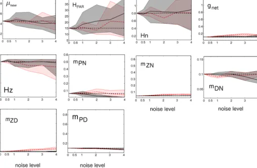
Figure 4. Uncertainties of the estimated parameters as a function of noise added to the synthetic “observations” (underlying the respective parameter optimizations). The magnitude of noise is expressed, as defined in Sect. 2.5. Typical observations correspond to level 3–4 noise (Sect. 2.5). The subplots refer to respective model parameters, indicated by the panel’s legends. Theyaxis limits match the associated parameter range explored (Table 1). The straight black dashed line refers to the original parameter values (that underlie the genuine truth).

The black lines refers to the ensemble mean retrieved by optimization. The grey shaded areas depict the ranges enveloped by all of the five ensemble members that constitute the parameter retrieval experiments at respective noise levels (NOISE). In all cases shown here the external forcing is OPTI. The red lines and red shaded areas are similar to the solid black line and grey shaded area, except that they refer to MISSING-ZD (as described in Sect. 2.5).

Figure 5. Temporal evolution of the model–data misfit (Eq. 9).

The model–data misfit measures the difference between the genuine truth and a simulation where the “truth” parameter set (Table 3) is modified by multiplyingH_N,H_PARandµby 4, 3 and 3.6, respectively. The black (red) line refers to simulations driven by OPTI (SENSI).

Table 4. Costs (range enveloped by all five ensemble members) for differing noise levels in the NOISE experiments (mmol Nm⁻³).

Two outliers were discarded.

Noise level Cost Genuine truth cost

0.5 0.041–0.042 0.043

1 0.084–0.087 0.086

2 0.171–0.173 0.172

3 0.254–0.258 0.258

4 0.334–0.339 0.344

This finding is confirmed by an exaggerated example in Fig. 5, which illustrates the difficulties in estimating the MM parameters on the one hand and their influence on the model’s sensitivity on the other hand. We compare the genuine truth to a simulation whereH_PAR, andH_N are strongly increased – much more than usually permitted (H_N is increased by a factor of 4,HPAR by a factor of 3). In a second step,µnew(µnew=3.6) was chosen to match the genuine truth as close as possible under forcing conditions OPTI. De- spite the extreme changes of the MM parameters, the simulation is relatively similar to the genuine truth (Fig. 5; black line). This, however, does not apply when switching to forcing data set SENSI (red line in Fig. 5), which leads to very different model behaviour. We conclude that the MM parameters are particularly hard to constrain and that their estimate depends strongly on the forcing data set used during the optimization process while, at the same time, they are key to the model’s sensitivity.

The problem with NOISE

The major difficulty in estimating the MM parameters is, apparently, their strong dependency on the maximum growth rate of phytoplankton (and on one another). Hence, an in- creasedH_PAR or H_N can be compensated to a large extent by choosing a larger appropriate valueµ_new. Figure 6a il-

(10)

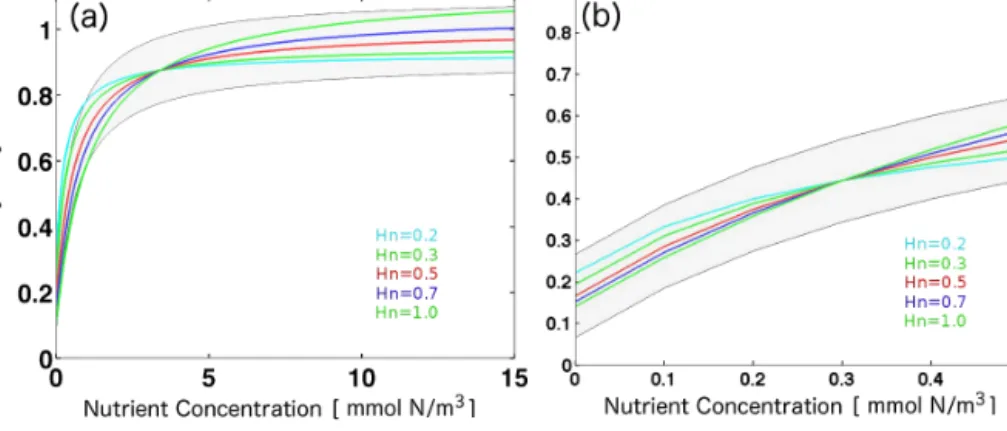
Figure 6. Normalized Michaelis–Menten curves (α_N+H^N

N) for various half-saturation constantsH_N, as indicated in the figure legends. The normalization constantαis chosen such that all curves cross at the same nutrient concentration. Panel (a) and (b) feature nutrient crossover concentrations of 4 and 0.3 mmol Nm⁻². Shaded areas envelope theH_N=0.5 curve by adding a constant value of±0.1 to this curve.

lustrates this compensation. It shows various MM curves describing nutrient limitation for various half-saturation constants,H_N. The curves are normalized such that all curves cross at a nutrient concentration of 4 mmol Nm⁻³ (which corresponds to a normalization ofα= ⁴

4+0.5/_4+H⁴

N). This illustrates that, by normalization, all curves can be (roughly) squeezed into an±0.1 envelope around theH_N=0.5 curve (gray shaded area). Such a compensating normalization of the actual phytoplankton growth (µmax PAR

PAR+H_PAR· ^N

N+HN) for distinct MM parameters can be easily achieved by changing the maximum growth of phytoplankton (µ_adapt=µmax·α) accordingly. In our setup, we find for every choice ofHN a µadaptsuch that the overall phytoplankton growth is changed by typically less than 10 % relative toH_N=0.5.

The extent to which a 10 % change of the overall phytoplankton growth effects a deviation from the genuine truth is, naturally, dependent on the choice (or retrieval) of the other parameters. By performing Monte Carlo simulations (as described in Appendix B) we derive a measure that is representative for the whole range of parameters (as listed in Table 1):

a change of ±10 % of the actual phytoplankton growth results in a mean change of the cost function of less than 8 %.

Reverse reasoning implies that, on average, a precondition for detecting a change of±10 % in the actual phytoplankton growth is a cost function which can be determined with a precision higher than±8 %. This is, however, unrealistic given the typical noise levels inherent to observations.

In summary, we conclude that in the presence of even only modest noise different settings of the MM parameters (within the permitted range, Table 1) can not be distinguished from one another – if the maximum growth rate of phytoplankton is changed accordingly. Note that the level of potential compensation between MM parameters and maximum phytoplankton growth depends on the forcing and gets more ef- fective as the range of nitrate variations decreases (Fig. 6b).

This implies, in turn, that the smaller the nitrate variations in

the forcing data set used for parameter estimations, the larger the difficulties to retrieve the MM parameters.

3.3 MISSING-ZD, SPARSE1, SPARSE2

Per se sparse data are, surprisingly, not problematic. As mentioned in Sect. 3.1, a variation of experiment EASY with monthly samples of standing stocks succeeded in retrieving the genuine truth parameter set by optimization. Under real- world conditions, however, sparse and irregular sampling is typically accompanied by noise and some prognostic variables may even be not observed at all (e.g. detritus, zooplankton).

The effect of unavailable observations of Z and D, in combination with noise added to P and D, is illustrated by the red shaded areas in Fig. 4. (The experimental setup corresponding to these illustrations is identical to the setup used to plot the gray shaded areas, except that zooplankton and detritus are not incorporated in the cost (experiment MISSING-ZD)).

In MISSING-ZD, the estimates of most parameters worsen and this holds especially for the retrievals of the parameters included in the zooplankton growth equation (Eq. 3). Inter- estingly, this does not hold for the MM parameters (andµnew, which is not independent as described above) where the inclusion of D and Z observations into the cost function is of no benefit for the parameter retrieval – on the contrary, it appears as if the inclusion of Z and D “dilutes” the relevant information in the cost function and the detailed information about Z and D adds unnecessary, and potentially misleading, information for the estimation of the MM parameters.

Another real-world problem is sparse data in time such as e.g. a seasonal bias in the number of available observations. Often, the data coverage is characterized by strong seasonal differences. The experiments SPARSE1 and SPARSE2 are designed to explore this. In both cases “level 1” noise is added. SPARSE1 is based on subsamples originating mainly

(11)

from autumn. SPARSE2 uses in addition observations from late winter and spring (cf. Fig. 2).

A technical detail is that our optimization algorithms seem to be more prone to converge towards a local minimum associated with relatively high cost when sparse observations are used. As a consequence we had to discard one estimate during experiment SPARSE1 and two estimates during experiment SPARSE2 (where the cost exceeded 0.2). Apart from this technical issue we find that SPARSE1 leads to surprisingly good parameter estimates, i.e, only slightly worse than the estimates obtained in MISSING-ZD, perturbed by noise at the same level, even though the data coverage is sparse.

SPARSE2, even though based on more data and generally associated with lower costs, shows no overall improvement. To the contrary, the estimated parameters related to zooplankton grazing are further away from the genuine truth parameters than in SPARSE1 (Table 3). In particular, the estimates of gnew, mZNandmZD worsen considerably (while the ensemble mean estimate ofm_PNandµ_newimprove). Some deviations are substantial; e.g. some retrievals ofg_newexceed the genuine truth parameters by more than 2.5-fold and some retrievals ofm_ZDexceed the genuine truth parameters by more than 10-fold.

These increases are not independent from one another. The parameter estimates ofµ_newandg_maxare correlated in the repeated experiments (correlation coefficient 0.5 which is sta- tistically significant, chance probability<0.05). Correlation coefficients betweenµnewandmDN are 0.96, while the correlation coefficients betweengmaxandmZD(mZN) are even higher (0.98 and 0.99, resp.).

This illustrates that many parameters are not independent of one another – in addition to obvious pairs such as growth and loss terms, and the ones described in Sect. “The problem with NOISE”. These additional (compensatory) dependencies are the consequence of constraining parameters with standing stocks, as is common practice.

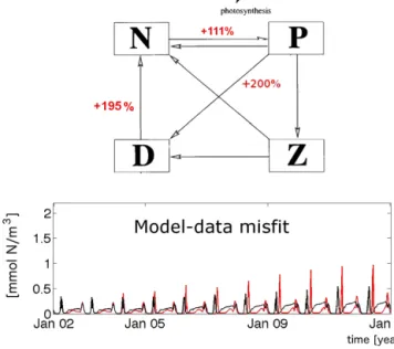
Standing stocks alone do not contain information on resi- dence times of the “base currency” nitrogen in the prognostic components. What they do contain is (only) information on the difference of in- and out-going fluxes, as changes in standing stocks are determined by variations in the difference of in- and out-going fluxes. When changing both in- and out- going fluxes by the same amount, the standing stocks will not be affected. Hence standing stocks are not necessarily affected by accelerated or decelerated nutrients cycles. This causes dependencies among e.g.µnewandmDN, as described above. Figure 7 shows an example where an increase ofmDN

can, in large part, be compensated as regards its effect on the cost by increasingµ_new andm_PDaccordingly (even though the model structure is non-linear). Increasing all three parameters results in a strongly increased N-P-D loop (up to 200 % as indicated by the red numbers) and, at the same time, in a simulation of all prognostic variables that is very similar to the genuine truth. Another example is the optimization study (based on real-world observations) of Oschlies and Schartau

Figure 7. Potentially small effects of cycle speed – an example.

Here, we compare simulations which differ from the genuine truth in that they feature increased fluxes among the compartments as indicated by the red numbers in the upper panel. The original parameter values are listed in Table 3 (column 2). The lower panel shows the temporal evolution of the difference (Eq. 9) between the genuine truth and the simulation with increased cycling. The black (red) line refers to simulations driven by OPTI (SENSI).

(2005) who found a comparable model–data misfits among two model versions which featured a factor 2.5 difference in primary production. Consistently, Friedrichs et al. (2007) report “different element flow pathways” for similar model–

data misfits.

The problem with SPARSE

The comparison of the parameter retrieval experiments SPARSE1 and SPARSE2 illustrates that the timing of the observations is relevant because not all times of the year contain information for the estimation of all parameters: SPARSE2 contains predominantly late winter and spring information which improves the estimates of some phytoplankton growth parameters. For all other parameters, however, the strong seasonal bias in SPARSE2, i.e. the underrepresentation of the second half of the year in the cost, seriously hampers their successful retrieval. Figure 8 illustrates this in detail. Appar- ently, the periods that contain information about the limiting effects of light and nutrients, i.e. about the MM parameters, are very short. The “information containing” period forH_PAR (dark yellow patch in Fig. 8) starts in spring when the surface mixed layer shoals to less than the “critical depth” (Sverdrup, 1953). It ends as nutrient limitation kicks in (which at the same time denotes the start of the “information containing”

period forH_N). Note that the changes in PAR incorporated by the dark yellow patch are only a fraction of the full amplitude

(12)

Figure 8. (a) Seasonal cycle of nutrient and light limitation of phy- toplankton growth (second year of the genuine truth simulation driven by OPTI). The MM term for light _PAR+H^PAR

PAR and nutrients N

N+HN are denoted by a yellow and blue line, respectively. (b) Cor- responding seasonal cycle of phytoplankton (green line), zooplankton (red line) and detritus (grey line). Shaded areas mark periods where the system is limited predominantly by light (yellow area) and by nutrient (brown area) before the zooplankton dynamics start to dominate the system. The dark yellow shaded area depicts light- limited periods in which there is net phytoplankton growth.

of the season cycle. The “information containing” period for HN (dark brown patch in Fig. 8) ends when the dominant control is exerted by top-down controlling Z.

Likewise, the information content about the other parameters is not equally distributed throughout the year. For example, the information about the zooplankton growth parameters is most pronounced in summer, when high abundances prevail. Obviously, loss rates are hard to assess during times when the respective prognostic variables are close to the limit of detection.

3.4 OBS10, OBS4

Real-world observations are typically sparse as regards time, space and sampled variables. In addition they are noisy.

Hence, by using real-world observations we face a combination of the problems described in the Sects. 3.2 to 3.3. We use quality checked data with a rather unusual high data coverage – but still data gaps exist and the noise level is con- siderable (Sect. 2.4). The typical noise level inherent to our real-world observations, approximated by the standard deviation of observed P from July to December amounts to 0.4 mmol Nm⁻³ which corresponds to a “level 3–4 noise”

as defined in Sect. 2.5. Since we use real-world observations now (and no genuine truth), the “true” parameter set is unknown and we compare different parameter estimation strategies with one another. From the lessons learned above, we expect a similar model performance when estimating all free parameters simultaneously (OBS10) and when estimating only the subsetµ,m_PD,m_DNandg_new(OBS4) because

– the MM parameters andH_z can not be constrained in the presence of noise (Sect. 3.2), i.e. one choice is as

good as another given that the remaining parameters are adjusted accordingly.

– the effects of changes inµmaxcan be compensated by a similar change ofmPN. Hence, given the noise level and probable model deficiency, they can not be constrained simultaneously,

– the observational data do not contain information about Z and D and we thus do expect that prescribing the loss rates of Z (mZD andmZN) will not worsen the model–

data misfit considerably.

Given the lower degree of freedom in OBS4, we expect in addition that the global minimum will be easier to detect.

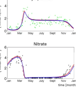
We find that indeed all speculations hold: when optimizing 10 parameters, repeated parameter retrievals lead to different parameter estimates associated with almost equal cost, while for OBS4 repeated optimization leads to strikingly similar parameter estimates. Figure 9 shows the simulations based on the “best” parameter estimates of OBS10 and OBS4, corresponding to costs of 0.764 and 0.783 mmol Nm⁻³, respectively. Because the difference between the two simulations is much smaller than the misfit of each of the simulation to the (noisy) observations, we conclude that it is impossible to judge which parameter set performs better.

4 Discussion

This study adds to the ongoing discussion about the problems of constraining all the parameters of state-of-the-art pelagic ecosystem models simultaneously (e.g. Ward et al., 2010; Schartau, 2003; Matear, 1995; Spitz et al., 1998; Rück- elt et al., 2010). By design, we can disentangle some of these potential problems: by using “twin experiments” (or, in other words, a subsampled synthetic “truth” rather than real-world observations), we can rule out the effects of a potentially deficient model formulation. Hence, we know that our problem is not ill-posed as regards the underlying equations, non-resolved processes or uncertainties in the external forcing and boundary conditions other than we willfully in- troduced. (Note that, even so, no unique solution may exist.) Furthermore, the twin experiment approach gives us full control over the “observations”, i.e. we can adjust the sampling (with respect to both, variables and time) and the noise inherent to our “observations” at will. The advantages of this approach have been appreciated in previous studies already (e.g. Friedrichs, 2001; Gunson et al., 1999; Law- son et al., 1996; Schartau et al., 2001; Spitz et al., 1998).

One major difference here, however, is the usage of reddish noise. Previous studies focused on data sampling, ne- glecting any noise or using white noise, to mimic errors in the observational data. The difference in the noise structure is essential. The impact on the optimization differs probably because red noise differs from white noise as there is

(13)

Figure 9. Real-world observations from station BY5 (55.15^◦N, 15.59^◦E; dots) and model simulations (lines). The red (blue) line refers to a model simulation integrated with the optimized parameter set retrieved during experiment OBS10 (OBS4).

more variance associated to timescales (days, seasonal to in- terannual) that are resolved by a typical ecosystem model.

Thus, an optimization procedure is more prone to sense a relation between noise-induced cost and parameter choice.

Consequently, low-frequency noise disrupts parameter estimation much more than white noise, which is in line with the findings of Friedrichs (2001), who rates systematic biases as much more detrimental than the presence of white noise.

Note that our definition of noise is broadened as it does not only include measurement accuracy but refers to noise effected by the combination of all unresolved processes that can cause deviations between simulated and observed values. Noise amplitude and structure that come along with this broadened definition of noise are hard to assess and we are not aware of any studies giving guidance on this. For the time being we assume reddish noise, which is typical for ocean processes (Hasselmann, 1976). As regards typical noise am- plitudes we find that the median of the relative standard error of all surface nitrate concentrations in the global monthly cli- matology of Garcia et al. (2010) is 20 %.

Returning to our experiments, we find that even a fraction of these typical noise levels does already prevent any meaningful parameter retrieval, as illustrated in Sect. 3.2. The reason is that noise at this level can open up “spurious” minima which are associated with a cost lower than the cost associ- ated with the genuine truth simulation. Such “spurious” minima are often related to very different parameter values than the genuine truth and might either be distortions of the minimum related to the genuine truth or minima opened up in addition. Note that such difficulties were not reported by earlier studies using twin experiments disrupted by white noise.

We conclude that the structure of the noise is relevant.

The parameter set associated to a spurious minimum may well imprint differing sensitivities when the external forcing is changed (Sect. 3.2, Fig. 3) and the overall behaviour of such a model reminds of extrapolation with an overfit- ted polynomial. In agreement with the early supposition of Matear (1995), who used real data and calculated the error- covariance matrix (via inversion of the Hessian matrix), we can relate major problems back to parameter dependencies.

Here we broaden the common definition of “parameter dependencies” and refer to changes in a certain parameter that can, in large parts, be compensated by changing other parameters accordingly. Such dependencies are reflected by high correlations of some parameter estimates in repeated runs.

Note, however, that the level of compensation depends on the forcing conditions.

To our knowledge, however, there is no technique to ex- amine all dependencies in a formal and useful way for the task at hand. Typical approaches such as correlation analy- sis or those based on analysing the Hessian matrix (as e.g.

Fennel et al., 2001; Kidston et al., 2011), have, in our con- text, their limitations because the dependencies are manifold and include up to four-way-parameter interactions. The Hes- sian matrix is designed to detect mutual dependencies between two parameters. Furthermore, it is a function of the model forcing and boundary condition and of the choice of the underlying parameter set, because it is a local derivative.

We, however, are interested in more generalized findings. We thus have to rely on the model structure and illustrative exam- ples to illustrate dependencies. Besides the obvious potential compensations of growth and loss terms, such dependencies occur e.g. in the growth term of phytoplankton (and similarly in the growth term of zooplankton). Other strong dependencies are a consequence of optimizing the model parameters with standing stocks. Since standing stocks are not necessarily affected by accelerated or decelerated nutrients cycles, all loops in the model structure contain strong parameter dependencies (Fig. 7).

A large part of the problems, associated with the parameter retrievals in the presence of noise, can be traced back to the Michaelis–Menten formulations which determine most of the model’s sensitivity to the external forcing (Sect. 3.2, Fig. 5). This finding is in agreement with Friedrichs et al.

(2006), who point out that the half-saturation constant for nutrients appears highly correlated to the maximum phytoplankton growth rate. Surprisingly we find that even an ex- traordinarily well sampled, full seasonal cycle of prognostic variables does not contain enough information to constrain the sensitivity of an N–P–Z–D model such that it can unambiguously project system dynamics in e.g. a warming world. In a nut shell, the reason is that only short periods are predominantly controlled by actual nutrients and/or light de- pleted conditions (Fig. 8). Generally these periods are not ended by replete conditions but by other dominating processes such as e.g. top-down control of zooplankton. This means that the information, which is relevant for parame-

(14)

ter optimization, within a seasonal cycle is rather limited, despite its apparently large variations in light and nutrient availability, and is generally not sufficient to constrain the systems’ behaviour e.g. under anticipated climate change.

Thus, laboratory experiments might be required to test the behaviour of ecosystems on anticipated future changes in the environmental conditions and to test and calibrate our models. An additional (somewhat related) problem is that a realistic (i.e. within the bounds spread by typical observational errors) simulation of standing stocks does not ensure a cor- rect cycling speed among prognostic variables (Fig. 7). It is important to note that, by making the model more complex, the above described problems do not disappear; on the contrary, additional problems are prone to emerge. Hence, more sophisticated observations such as rates or fractionating iso- topes are mandatory for constraining fluxes or transfer rates among the prognostic variables.

5 Summary and conclusions

To date, parameters associated with biogeochemical pelagic models, coupled to 3-D ocean circulation models, are, more often than not, assigned by rather subjective parameter tun- ing exercises. It seems straightforward to assume that automated numerical optimization procedures which minimize some quantitative measure of the deviation between observations and their simulated equivalents are more objective and thus represent a reliable procedure for parameter alloca- tion. In the past, such an approach was barred by excessive computational demands. Recent advances in so-called offline approaches (Khatiwala, 2007, 2008; Kriest et al., 2012) and optimization procedures (Prieß et al., 2013) have severely re- duced the demands and pushed the tasks within reach.

However, per se, it is unclear how far such approaches will carry, even if the underlying model equations were exact. Our study provides some insight by applying optimization procedures which minimize a generic cost function (root mean squared errors) based on a synthetic set of “observations”, which was produced by sampling our simulation at specific times. Differing levels of artificial noise were added to the synthetic “observations” to mimic typical real-world conditions. By mimicking sampling strategies and noise inherent to the observations we systematically explored what kind of observations are required to retrieve the parameters of the

“genuine truth” simulation by parameter optimization. This

“twin experiment” approach (as it is often referred to) gives guidance on the question what kind of information, or model parameters, can be extracted from observations. The caveat here is that we implicitly assume that the underlying mathematical equations are exact – certainly an overoptimistic assumption since the equations are not derived from first principles (cf. Smith et al., 2009).

Our exercises suggest that monthly observations of all prognostic variables are sufficient to retrieve the actual model

parameters correctly. However, this does not hold if the observations are defiled by noise. Even modest noise levels (≈10 %) can already lead to minima in the cost functions which are associated to a lower cost than the genuine truth simulation. We find that these minima develop due to strong parameter dependencies, or rather their potentially compensating effects when other parameters are changed accordingly. Such dependencies occur e.g. in the growth term of phytoplankton and in circular parts in the model structure.

The implication is that, in the presence of noise, the optimal parameter set in terms of cost is not necessarily the cor- rect one. This is of concern because we find that, although the optimal solution and the genuine truth are similar under the given external forcing, they can feature very diverg- ing behaviour, once the forcing is adjusted within the envelope of e.g. anticipated changes in the Baltic Sea. Most of this behaviour is apparently caused by the poorly constrained Michaelis–Menten (MM) parameters which are commonly used to describe nutrient and light limitation of phytoplankton growth (Fasham et al., 1993; Yool et al., 2009; Dutreuil et al., 2009; Oschlies et al., 2010), although the MM formulation is controversial (Smith et al., 2009).

Other than noise, we find that typical characteristics of real-world observations such as irregular sampling in time or the absence of observations of simulated prognostic variables such as e.g. zooplankton and detritus do also seriously ham- per attempts to retrieve all model parameters simultaneously (Fig. 4). An exception to the latter rule are the MM parameters which are apparently easier to constrain when zooplankton and detritus observations are not part of the cost function.

Hence, more data are not necessarily better data. The inclusion of more data in the cost function might even degrade the ability to constrain certain parameters.

As regards real-world conditions (where only noisy and irregularly sampled data of some prognostic variables are available to assemble some quantitative measure of model performance) our findings suggest a sequential, two-step approach, starting with an estimation which focuses on the MM constants and to take care that the measure of model performance contains relevant information only. This applies both to sampled variables and to sampling time interval and should prevent unnecessary “dilution” of information which is vital because the parameter estimation is so sensitive to noise. For example, it does not make sense to constrain MM constants which determine growth limitation with data characterized by a period of plenty or with observations of D and Z. Furthermore, the larger the range of sampled conditions, the higher the probability of retrieving meaningful model parameters. A cross-validation with a second independent data set as a last step can increase the confidence in the model further (Gregg et al., 2009).

Our experiments with real-world observations imply that the other parameters may be estimated in a second step during which the MM parameters are held constant to a priori values. This approach is seemingly in line with earlier stud-