1. Introduction
The mass loss of the Greenland Ice Sheet increased from 41 ± 17 Gt/year in 1990–2000 to 286 ± 20 Gt/year in 2010–2018 (Mouginot et al., 2019). During the period 1972–2019, Humboldt Gletscher lost 161 billion tons (Gt) of mass, i.e. the fourth largest contribution behind Jakobshavn Isbræ (335 Gt) in central west, Steenstrup/Dietrichson (230 Gt) in north west, and Kangerlussuaq (174 Gt) in east Greenland. Humboldt is also the widest glacier in Greenland at 100 km, with slow motion (100 m/year) in shallow waters (150 m) in its southern half and faster motion (200–600 m/year) in deeper waters (300 m) in its northern half (Fig- ure 1). Its balance flux, i.e. the average surface mass balance (SMB) for the years 1961–1990, is 2.0 Gt/yr.
Ice discharge increased from 4.8 Gt/year in the 1970s to 6.7 Gt/year in 2019, hence the glacier was out of balance the entire period. Its 48,623-square-km basin holds enough ice to raise sea level by 19 cm, i.e. the 10 largest reserve of ice in Greenland. The glacier is grounded below sea level along its entire front. In the north, a submarine channel extends into the interior (Morlighem et al., 2017). The glacier had a small float- ing section along its northern flank in the 1990s (Rignot et al., 2001).
A leading hypothesis for the evolution of Greenland's glaciers is that the enhanced intrusion of warm At- lantic Intermediate Water (AIW) in the fjords in the 1990s melted the glacier fronts, de-stabilized them, and increased mass discharge (Catania et al., 2019; Christoffersen et al., 2011; Holland et al., 2008; I. M. Howat et al., 2008; Murray et al., 2010). Few ocean and depth measurements have been available to quantify water temperature in the fjords, which makes it difficult to interpret the changes. The International Bathymetric Chart of the Arctic Ocean version 3.0 (IBCAO Ver. 3.0) did not include quality bathymetry in the fjords
Abstract
Humboldt Gletscher is a 100-km wide, slow-moving glacier in north Greenland which holds a 19-cm global sea level equivalent. Humboldt has been the fourth largest contributor to sea level rise since 1972 but the cause of its mass loss has not been elucidated. Multi-beam echo sounding data collected in 2019 indicate a seabed 200 m deeper than previously known. Conductivity temperature depth data reveal the presence of warm water of Atlantic origin at 0°C at the glacier front and a warming of the ocean waters by 0.9 ± 0.1°C since 1962. Using an ocean model, we reconstruct grounded ice undercutting by the ocean, combine it with calculated retreat caused by ice thinning to floatation, and are able to fully explain the observed retreat. Two thirds of the retreat are caused by undercutting of grounded ice, which is a physical process not included in most ice sheet models.Plain Language Summary
Humboldt Gletscher is the widest glacier in Greenland, slow moving, and terminating in shallow waters in its southern half, but grounded 200 m deeper than previously known in its northern half, with a submarine trough extending more than 100 km inland. The glacier has been retreating at 0.6 km/year and contributing significantly to sea level rise. We attribute the retreat to undercutting of grounded ice by warmer ocean waters combined with a retreat caused by ice thinning to floatation sooner due to glacier speed up. The glacier, which hosts an ice volume equivalent to a 19-cm global sea level, will remain a major contributor to sea level rise this Century.© 2021. The Authors.
This is an open access article under the terms of the Creative Commons Attribution-NonCommercial License, which permits use, distribution and reproduction in any medium, provided the original work is properly cited and is not used for commercial purposes.
Eric Rignot1,2 , Lu An1 , Nolwenn Chauche3 , Mathieu Morlighem1 , Seongsu Jeong1 , Michael Wood1,2 , Jeremie Mouginot1,4 , Josh K. Willis2 , Ingo Klaucke5 , Wilhelm Weinrebe5, and Andreas Muenchow6
1Department Earth System Science, University of California Irvine, Irvine, CA, USA, 2Jet Propulsion Laboratory, California Institute of Technology, Pasadena, CA, USA, 3Access Arctic SARL, Le Vieux Marigny, France, 4Institut des Geosciences de l'Environnement, Universite Grenoble-Alpes, CNRS, Grenoble, France, 5GEOMAR Helmholtz Centre for Ocean Research Kiel, Kiel, Germany, 6School of Marine Science and Policy, University of Delaware, Newark, DE, USA
Key Points:
• The 100-km wide Humboldt Gletscher holds a 19-cm sea level rise equivalent, lost 161 billion tons of mass, and retreated 13 km since
• Warm waters at 0°C flood a 350–1972 400 m deep trough on its northern flank that remains below sea level more than 100 km inland
• We explain the glacier retreat as 70%
from ocean-induced undercutting and 30% from thinning-induced retreat
Correspondence to:
E. Rignot, erignot@uci.edu
Citation:
Rignot, E., An, L., Chauche, N., Morlighem, M., Jeong, S., Wood, M., et al. (2021). Retreat of Humboldt Gletscher, north Greenland, driven by undercutting from a warmer ocean. Geophysical Research Letters, 48, e2020GL091342. https://doi.
org/10.1029/2020GL091342 Received 6 NOV 2020 Accepted 21 JAN 2021
Geophysical Research Letters
(Jakobsson et al., 2012), making it difficult to understand how warm, salty, subsurface (depth >350 m) could reach the glaciers.
In 2015, NASA launched the Ocean Melting Greenland mission (Fenty et al., 2016) to collect multi-beam echo sounding (MBES) data by ship, airborne high resolution gravity, airborne surface topography, air- launched Airborne eXpendable Conductivity, Temperature, and Depth (AXCTD) probes and traditional ship-based CTDs (An et al., 2019; Wood et al., 2018). The data were used to reconstruct glacier thickness and bed elevation from mass conservation with constraints from MBES data, which is BedMachine v3 (BMv3) (Morlighem et al., 2017) and IBCAO Ver. 4.0 (Jakobsson, Mayer, Bringensparr, et al., 2020). The data set provides a smooth and reliable transition in bed elevation at the glacier front, which is critical for ice sheet models. BMv3 provided a major revision of glacier depths, with bed elevations several 100 m deeper than previously known. Greater water depth in the fjords means more exposure to AIW, which is confirmed with AXCTD data in most fjords (Fenty et al., 2016).
Glaciers draining north Greenland have not been surveyed in detail. The front of 79°N was surveyed in 2016;
Ryder fjord in 2019 (Jakobsson, Mayer, Nilsson, et al., 2020) and Peterman in 2016 (Jakobsson et al., 2018).
These glaciers hold a large potential for sea level rise because they drain submarine basins. These northern glaciers have been protected from decay by buttressing ice shelves, consolidated by the presence of a thick sea ice melange which glues ice blocks together, but this melange has decayed in recent decades (Hig- gins, 1991). Many floating sections have retreated or disappeared: Zachariae Isstrøm, Humboldt (discussed herein), Hagen Bræ, and Ostenfeld (Moon & Joughin, 2008).
Here, we present the results of an oceanographic survey of Humboldt Gletscher (named Humboldt in the remaining of the paper) conducted in the summer of 2019 with MBES and CTD data along its ice front, combined with remote sensing data going back to 1970s and CTD data going back to the 1960s. We employ the results to interpret the glacier evolution over the last 6°decades. We conclude on the role of the ocean in melting this major glacier of north Greenland.
2. Data and Methods
2.1. Background
The 100-km wide Humboldt Glacier (also named Sermersuaq) is the widest glacier in Greenland (Weid- ick, 1995). It drains into Kane basin, a broad channel that connects Baffin Bay to the South and Nare Straits to North. First discovered in 1853 by Elisha Kent Kane, first explored by Lauge Koch in 1912–1913, the first
10.1029/2020GL091342
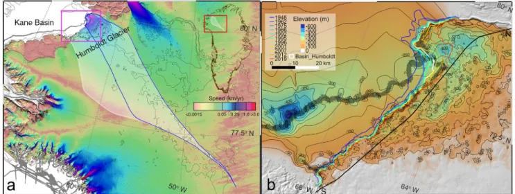
Figure 1. Humboldt Gletscher, Greenland, with (a) drainage basin in shade white (blue outline is the northern half of the basin) overlaid on color-coded ice speed from brown (no motion) to red (greater than 3 km/year) on a logarithmic scale; inset (red) of the basin in Greenland, and of area (purple) in Figure 1b;
(b) bathymetry in front of and beneath the glacier with 50-m contour levels below sea level. Ice front positions from 1948 (blue) to 2019 (red). Ice thickness profile S-N for ice fluxes and thinning rates in Figure 2 (Mouginot et al., 2019). Gray areas in (a) and (b) indicate bathymetry data.
modern frontal position of Humboldt dates from 1948 (Hill et al., 2018) (Figure 1). The numerous lakes and drainage channels in its ablation zone suggested a relatively low level of motion causing low crevassing. The glacier front is flanked by tabular icebergs, especially in the north, i.e. bergs than are wider than taller which are typical of cold regions like Antarctica. Icebergs farther south are taller than wider and tend roll over when detached from the ice front. Tabular icebergs drift away from the ice front and get stranded on shal- lower areas for many years. Ice thickness near the terminus varies from 250 to 300 m in the south to 350–
600 m in the north (Figure 2). There are few prior glaciological studies of Humboldt (Carr et al., 2015; Hill et al., 2018; Joughin et al., 1999, 2010; Livingstone et al., 2017; Mouginot et al., 2019; Rignot et al., 2001).
Because of its slow flow and moderate thickness, its ice discharge is 10 times less than for Jakobshavn Isbrae and 3 times less than for Petermann Gletscher (Mouginot et al., 2019). Despite that, Humboldt holds an ice volume equivalent to a 19-cm global sea level rise.
2.2. Dynamic Thinning
We combine ice thickness and velocity data to update the ice fluxes from 1972 to 2019 along a S-N thickness line located a few km upstream the ice front (Mouginot et al., 2019) (Figure 1). Changes in ice elevation, used to correct ice thickness (Figure 2), are derived from a 1978 digital elevation model (DEM) (Korsgaard et al., 2016), Airborne Topographic Mapper data from 1993 to 2016 (Krabill, 2004), ICESat data from April 2004, Greenland Ice Mapping Project (GIMP) DEM from January 2006 (NSIDC-0645), and January 2011 (NSIDC-0715) (I. Howat et al., 2014), time-tagged ArcticDEMs from October. 2015 (Porter et al., 2018), and ICESat-2 data from June. 2019. For years with no measurement, we interpolate the elevation from the nearest measurements in time and space using triangular irregular networks. We use ICESat-2 ATL06 altimetry data version 2 (Smith et al., 2020), filter outliers by comparing the ATL06 profiles with GIMP (I.
Howat et al., 2014) and eliminate points more than 80 m away to produce a 1-km DEM. We estimate the height bias of the DEM on ice-free land from a comparison with other DEMs. The lowest-noise difference map is obtained combining ICESat-2 and GIMP 2006, with a time difference of 13 years. The height bias is 3.4 ± 7 m. This thinning map helps re-calculate ice thickness using the mass conservation algorithm. In this algorithm, ice thickness is reconstructed in between direct measurements of ice thickness using the ice flow direction from remote sensing and applying conservation of mass in between thickness gates. The rates of Figure 2. Humboldt Gletscher, Greenland, (a) surface speed, and (b) surface elevation along ice-thickness profile S-N in Figure 1, color coded from 1979 (blue) to 2019 (red), and overlaid on bed topography with bedrock in brown and ice in gray, (c) cumulative anomaly in ice discharge, D, and surface mass balance, SMB, in Gt (gigaton = 1012 kg/year) from 1972 to 2019 in reference to a balance flux of 2 Gt/year for 1961–1990, and (d) air temperature (°C) at 80°N and 65°W (red) and runoff production (blue) (in Gt/year).
Geophysical Research Letters
thinning along the S-N profile are used to calculate the rate of thinning-induced grounding line retreat, qs, which reflects that thinner ice reaches flotation sooner.
2.3. Grounding Line Retreat
Ice front positions are digitized from the 1962 Declassified Intelligence Satellite Photography mosaic and the Landsat time series from 1975 to Landsat-8 in 2019. We calculate a mean glacier retreat rate in meters by dividing the area of retreat by the length of the ice front. We divide the glacier into two sectors: 1) the north- ern and 2) southern halves (Figure 1). We mapped the grounding line in 1992 and 1996 using ERS-1 data (Rignot et al., 2001), at which time we identified a small floating ice tongue 27.1 km2 in size in the north.
In 2017–2018–2019, Sentinel-1a/b at a 6-days repeat interval along Track026 reveal no grounding line. The small floating ice tongue disappeared between 1996 and 2017. Grounding line and ice front positions are assumed to coincide during the entire observation period.
2.4. Bathymetry
We collected MBES data onboard the M/Y Arii moana in August 2019 using the Helmholtz Center for Ocean Research Kiel SeaBeam 1050 multibeam echo sounder (MBES). The sonar was mounted on the bow of the boat 0.8 m below the water level. Correction for sound velocity (range calculation and ray-tracing) was performed using real-time sound velocity sensor mounted on the head of the transducers and CTD data collected at regular intervals (An et al., 2018) from an AML Oceanographic Minos X CTD. The Qinsy QPS and Cloud Compare softwares are used to process the MBES data. The bathymetry data is processed onto a regular grid at 25 m and displayed on top of IBCAOv3 (Figure 1).
In BMv3, mass conservation was applied to reconstruct glacier thickness (Morlighem et al., 2017) using Op- eration IceBridge ice thickness, a velocity map from 2007 to 2008 (Rignot & Mouginot, 2012), SMB for the period 1961–1990, and a map of ice thinning from Csatho et al. (2014). This configuration produces a bed solution that is not compatible with the 2019 MBES data. Instead, we use the ICESat-2/GIMP ice thinning product described to constrain elevation change. With this product, we are able to obtain a bed solution that matches the MBES data within 10 m. Without the ICESat-2/GIMP DEM the mass conservation algorithm is not able to converge with a solution that agrees with the MBES data.
2.5. Ocean Thermal Forcing
Air-launched AXCTD data were collected on a Grumman Gulfstream III aircraft in September/October 2016, C-130 Hercules in October 2017, a Basler DC-3 Turbo Prop in August/September 2018, and a Basler BT-67 in August/September 2019. During the ship survey, we collected traditional ship-launched CTD with an AML Minos-X probe. We combine the AXCTD data with historical CTD data from the Hadley center (bodc.ac.uk) spanning from 1960 to 2019 to document temperature changes. In Kane Basin, cold, fresh arctic waters flows southbound from Nares Strait in a western boundary current along Ellesmere Islands, along a 20–30 km wide, 250-m deep trough, before joining Baffin Bay at a narrowing named Smith Sound where the sea floor deepens to 500–600 m. A northerly, deeper flow of AIW takes place on the eastern side of Smith Sound, connecting with a southwest-northeast channel that extends to the front of Humboldt (Melling et al., 2001; Munchow & Melling, 2008; Munchow et al., 2015). A cyclonic circulation of ocean waters takes place in Kane Basin, which brings AIW in contact with Humboldt. In our analysis of ocean temperature, we only consider CTD data extending from the eastern side of Smith Sound to the front of Humboldt (Figure 3).
We calculate ocean thermal forcing, TF, as the depth-integrated difference between the temperature of the ocean and the pressure-dependent and salinity dependent freezing point of seawater. We divide the range of depths into 100 m segments overlapping by 50 m (hence 50–150, 100–200, etc.) and perform a linear re- gression of temperature versus time at each depth. We limit the CTD selection to the box in Figure 3 which coincides with the northerly flow of AIW toward Humboldt. If we use a larger box in Kane Basin, we find the same warming trend within 0.1°C. If we use a smaller box centered at the front of Humboldt Glacier, we find the same results with a larger uncertainty because there are less CTD data in front of the glacier.
10.1029/2020GL091342
2.6. Runoff and Undercutting
We use a reconstruction of runoff from RACMO2.3p2, to which we add meltwater production from basal sliding calculated from the UCI/JPL Ice Sheet System Model (Goelzer et al., 2020). Runoff averages 4.7 Gt/
year for 1961–1990 (Figure 2). Over 1958–2019, the cumulative anomaly in runoff totals 84.7 Gt. Runoff increased by 0.74 Gt per decade or doubled over the time period.
To calculate the rate of glacier undercutting, we employ the ocean model results in Rignot et al. (2016).
The rate of undercutting, qm, is the maximum rate of ice melt which takes place near the ice base. The ice above the incision is not supported by the bed and therefore exerts no basal resistance, while the ice below the incision is too thin to exert much buttressing. In effect, undercutting acts as a forced ground- ing line retreat of the glacier. Its rate depends on subglacial water discharge, water depth, and thermal forcing. All three variables are time dependent as a function of the position of the glacier front. Namely, Figure 3. Historical Conductivity, Temperature, Depth (CTD) data collected in Kane Basin, North Greenland from year 1961–2019 with (a) locations of casts overlaid on a (color coded) bathymetry within a yellow bounding box delineating where CTD data were selected to calculate ocean thermal ocean; (b) depth versus temperature for the corresponding CTD data color coded from blue to red; (c) temperature with 0.5°C contour levels and (d) salinity data with 0.2 psu contour levels along the continuous red dotted shown in the inset of Figure 3a with AXCTD locations for year 2019 as red filled circles. Red numbers indicate the depth of the seafloor at the CTD location.
Geophysical Research Letters
(0.0003 0.330.15) 1.18
m sg
q b q TF , where b is water depth in meters, qm
and qsg are in meters per day, and TF is thermal forcing.
In this study, we assume that the rate of grounding line retreat, qgl, is the result of the balance between ice advection, qf, and ice ablation (qm + qs + qc), i.e. qgl = qm + qs + qc − qf. At steady state, qgl = qs = 0 and qf = qm + qc. Starting from this steady state, we assume that the cumula- tive retreat over a time period, Qgl, is balanced by the cumulative retreat caused by undercutting, Qm, and cumulative thinning-induced retreat, Qs, i.e. Qgl = Qs + Qm, and the cumulative anomaly in advection is exactly compensated by the cumulative anomaly in calving, Qf = Qc, i.e. the gla- cier calves floating blocks of ice at the speed of advection.
3. Results
Annual ice discharge, D, averaged 4.2 Gt/year in 1972–2000, 4.4 Gt/year in 2000–2017 and peaked at 6.4 Gt/year in 2018. SMB decreased from near balance from the 1970s to −1.1 Gt/yr in 2000–2017. The mass loss increased from 1.9 ± 0.3 Gt/year in 1972–1990 to 5.6 ± 0.2 Gt/year in 2000–2017 for a cumulative 119 Gt for discharge versus 48 Gt for SMB.
Ice speed increased by 54% since 1972, with peak values ranging from 483 m/year in 1975 to 745 m/year in 2019 (Figure 2). The cumulative retreat Qgl peaked at 13 km in the north (Figure 1). The average retreat for 1962–2019 was 3.4 km, with 4.6 km for the northern half versus 2 km for the southern part Figure 4.
The revised bed elevation is 200 m lower at the ice front than in BMv3, with smaller corrections inland. The bed trough remains below sea level for more than 100 km (Figure 1). Prior estimates employed underesti- mated thinning which resulted in underestimated ice thickness and bed elevation at the ice front.
Using the NCEP/NCAR reanalysis data (Kalnay, 1996) at 80°N and 65°W, we find a 1.7°C warming in 1948–2020 for Humboldt. Most of the warm- ing occurred after 1991 (0.3°C cooling in 1948–1991 vs. 0.7°C warming per decade or 2.2°C in 1990–2020) (Figure 2). Runoff correlates strongly with warming (Figure 2d). Along the radar thickness line of Humboldt, the reference SMB averages −1 ± 0.2 m/yr. Over the time period 1958–
2020, the cumulative anomaly in SMB reached 8.6 ± 1.4 m along the ice front, with a peak at 13 m, versus an averaged thinning of 20 ± 23 m for 1978–2020, with a peak at 84 m. The observed thinning, which is much larger than that caused by surface melt, is therefore mostly of dynamic origin, i.e. enhanced glacier flow. To get subglacial discharge, qsg, we di- vide the runoff values by the glacier cross-sectional area below sea level, i.e. 16.3 km2 in 1962 versus 20.8 km2 in 2019 (12.7 for the north). We find 0.62 ± 0.2 m/d in 1960–1990 versus 0.98 ± 0.4 in 2000–2019.
Within the ocean box in Figure 3, ocean warming for 1960–2019 is 0.83°C at 50–150 m depth, 0.99°C at 100–200 m, 1.13°C at 150–250 m, 0.99°C at 200–300 m, 0.86°C at 250–350 m, 0.85°C at 300–400 m and 0.90°C at greater than 350, with a reference temperature increasing, respectively, from −1.43°C to −1.41°C, −1.34°C, −1.14°C, −0.99°C, −0.94°C, and −0.92°C (Figure 3). These temperature data are converted into TF versus depth using the pressure-dependent freezing point of seawater.
A transect of CTD from Baffin Bay to Nares Strait along Humboldt reveals warm AIW extending from Smith Sound to Humboldt (Figure 3). AIW originating from Baffin Bay has salinity of 34.4 psu versus 34.8 psu in
10.1029/2020GL091342
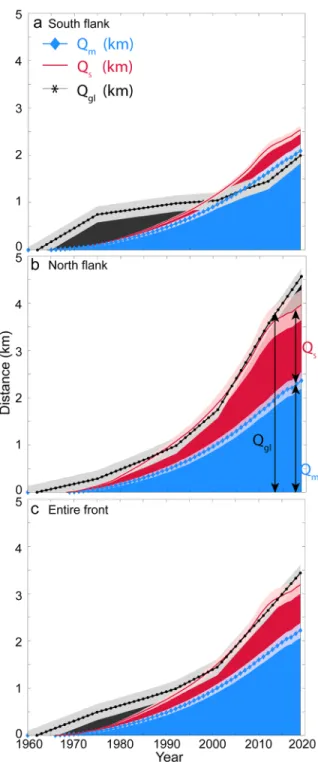
Figure 4. Cumulative grounding line retreat, Qgl, in kilometer (km) along the (a) South, (b) North, and (c) entire ice front of Humboldt (black) versus the cumulative retreat caused by ice thinning, Qs (red), on top of the cumulative retreat caused by undercutting from the ocean, Qm (blue) for the time period 1962–2019. If correct, the observed Qgl, in black, should match the sum of Qm and Qs represented in red, within error bars.
Nares Strait (Figure 2d). The water flow in Smith Sound is laterally sheared between southward flow in the west and northward flow in the east (Munchow & Melling, 2008). The northward flow does not extend into Kennedy Channel. Much mixing and recirculation takes place within the eastern Kane Basin on account of strong tides and shoaling topography.
Time series of TF, qsg, and water depth, b yield qm values increasing from 65 ± 4 m/year in 1960–1970 to 131 ± 12 m/year in 2010–2019. For the northern part, qm increased from 87 ± 5 m/year to 160 ± 18 m/year versus 48 ± 4 m/year to 108 ± 9 for the south. Hence undercutting doubled over the time period of investi- gation. While qsg is an important participant in qm, it contributes only 30% of qm. Most of the increase in qm
is caused by warmer ocean waters, as in Morlighem et al. (2019).
The calculated cumulative retreat Qm caused by undercutting totals 2.2 km for the entire front, 2.4 km for the northern half and 2.0 km for the southern half. For comparison, the observed ice front retreat Qgl to- tals 3.4 km for the entire front, 4.6 km in the north versus 2.0 km for the south. The retreat caused by the observed dynamic thinning of the ice front, Qs, is estimated at 1.0 km m for the entire front, 1.7 km for the north and 0.5 km for the south. When comparing the cumulative anomaly in ablation, Qm + Qs, with Qgl, we underestimate the observed retreat, Qgl, by +5% for the entire section, by −30% in the south, and +12% in the north, which is within our margins of error.
4. Discussion
The agreement between observed retreat, Qgl, and calculated retreat, Qm + Qs, has several implications.
First, ice thinning alone cannot explain the observed retreat. The retreat caused by ice thinning explains only 30% of the signal. It is necessary to invoke another physical process of grounded ice removal to explain the observed retreat. Second, ice thinning is mostly of dynamic origin (57%), i.e. glacier speed up. Enhanced surface melt contributes 43% of the thinning. Since thinning contributes 30% of the retreat, surface melt only contributes 13% of the observed retreat. Surface melt also contributes to the rate of undercutting, Qm, but to a lesser degree than the ocean temperature because the subglacial flux, qsg is scaled by a power 1/3 instead of 1.2 for TF, and qsg is only significant a couple of months per year. We conclude that our results suggest a strong contribution of a warmer ocean to the evolution of Humboldt. Third, the increase in the rate of undercutting explains 70% of the retreat. If these estimates are correct, undercutting is the dominant driver of the retreat, similar to what was found in northwest Greenland (Wood et al., 2018). We note that undercutting is overestimated in the shallow southern half where Qm + Qs exceeds Qgl by 30%. A similar overestimation was noted in northwest Greenland for shallow glaciers in cold waters. We attribute the over- estimation to the fact that the undercutting model was optimized from thicker glaciers standing in warm, salty, subsurface AIW.
The agreement between calculated and observed retreat suggests a posteriori that the calving of grounded ice blocks does not have an impact on the retreat of Humboldt Glacier, otherwise we would underestimate the observed retreat versus the calculated retreat, Qm + Qs, which is not the case. Indeed, Humboldt produc- es mostly tabular icebergs, recognizable as wide-shaped rectangles in satellite imagery, i.e. the ice blocks are already floating when they detach from the front. We conclude that our analysis, if correct, suggests that the calving flux, qc, essentially balanced the advection flux, qf.
The calving of ice blocks should not have contributed to the retreat of grounded ice because the calving of floating ice does not impact the retreat of a grounding line. Only the calving of grounded ice blocks could influence the glacier force balance via a reduction in basal friction. Humboldt produces mostly tabular icebergs, recognizable as wide-shaped rectangles in satellite imagery, i.e. floating ice blocks that detached from the front, already afloat. If Qc had increased significantly and started to calve off grounded ice blocks, we would find that the calculated retreat, Qm + Qs, would underestimate the observed retreat, which is not the case. This agreement between calculated and observed retreat suggests a posteriori that the calving of grounded ice blocks does not have an impact on the glacier retreat.
There are multiple sources of uncertainties in the estimates of undercutting, e.g. TF, water depth, model pa- rameters, but the results are robust to these uncertainties because we consider a long period of observations,
Geophysical Research Letters
hence the cumulative changes in elevation, ice front positions and TF are large compared to these uncer- tainties. Over shorter time periods, e.g. a decade, it would be more challenging to close the mass budget.
The new bathymetry confirms the presence of a deep channel underlying the northern sector of Humboldt that may be conducive to fast retreat. The retreat has been fueled by warm AIW that occupies a channel deeper than previously known. The disappearance of the small floating tongue observed in the 1990s coin- cides with the disappearance of floating tongues on Zachariae Isstrøm, Ostenfeld, and Hagen Bræ and the reduction in sea ice cover in the fjords (Reeh et al., 2001), hence is consistent with a broad pattern of ocean and air warming that has triggered a widespread and rapid retreat in north Greenland.
5. Conclusions
In this study, we present new bathymetry data in front of Humboldt Gletscher that make the bed topog- raphy 200 m deeper than previously reported at the ice front, hence more prone to vigorous melting from subsurface ocean waters and with a deeper bed channel to promote inland retreat. We review the climate forcing, air and ocean temperature and its effect on the glacier in terms of runoff, thinning, and retreat over the time period 1960–2019 and examine both the northern, deeper, faster part and the southern, shallower, slower part of this 100-km wide system. We compare the results with the retreat calculated from ice thin- ning, which results from ice dynamics and enhanced surface melt, and the retreat calculated from ocean undercutting, which depends on subglacial runoff, water depth, and water temperature. We find an excel- lent agreement between the observed retreat and that calculated from the components, but attribute more than 70% of the retreat to the action of ocean warming. We conclude that the ocean plays a major role in the glacial retreat. In the coming decades, the ocean will likely continue to play a large role in the glacier retreat.
Collectively, these results make Humboldt Gletscher a very important glacier to monitor in the future.
Data Availability Statement
Multibeam echo sounding data and AXCTD data are available at omg.jpl.nasa.gov. Ice velocity and mass balance data are in Mouginot et al. (2019) supplementary table.
References
An, L., Rignot, E., Millan, R., Tinto, K., & Willis, J. (2019). Bathymetry of Northwest Greenland Using “ocean melting Greenland” (omg) high-resolution airborne gravity and other data. Remote Sensing, 11(2), 131.
An, L., Rignot, E., Mouginot, J., & Millan, R. (2018). A century of stability of Avannarleq and Kujalleq glaciers, west Greenland, ex- plained using high-resolution airborne gravity and other data. Geophysical Research Letters, 45(7), 3156–3163. https://doi.
org/10.1002/2018GL077204
Carr, J., Vieli, A., Stokes, C., Jamieson, S., Palmer, S., Christofferson, P., et al. (2015). Basal topographic controls on rapid retreat of Hum- boldt glacier, northern Greenland. Journal of Glaciology, 61(225), 137–150.
Catania, G. A., Stearns, L. A., Moon, T. A., Enderlin, E. M., & Jackson, R. H. (2019). Future evolution of Greenland's marine-terminating outlet glaciers. Journal of Geophysical Research: Earth Surface, 125, e2018JF004873. https://doi.org/10.1029/2018JF004873
Christoffersen, P., Mugford, R. I., Heywood, K. J., Joughin, I., Dowdeswell, J. A., Syvitski, J. P. M., et al. (2011). Warming of waters in an east Greenland fjord prior to glacier retreat: Mechanisms and connection to large-scale atmospheric conditions. The Cryosphere, 5, 701–714.
Csatho, B. M., Schenk, A. F., van der Veen, C. J., Babonis, G., Duncan, K., Rezvanbehbahani, S., et al. (2014). Laser altimetry reveals com- plex pattern of Greenland ice sheet dynamics. Proceedings of the National Academy of Sciences, 111(52), 18478–18483.
Fenty, I., Willis, J. K., Khazendar, A., Dinardo, S., Forsberg, R., Fukumori, I., & others (2016). Oceans melting Greenland: Early results from NASA's ocean-ice mission in Greenland. Oceanography, 29(4), 72–83.
Goelzer, H., Nowicki, S., Edwards, T., Beckley, M., Abe-Ouchi, A. A., et al. (2020). Design and results of the ice sheet model initialisation experiments initMIP-Greenland: an ISMIP6 intercomparison. The Cryosphere, 12, 1433–1460.
Higgins, A. K. (1991). North Greenland glacier velocities and calf ice production. Polarforschung, 60(1), 1–23.
Hill, E. A., Carr, J. R., Stokes, C. R., & Gudmundsson, H. (2018). Dynamic changes in outlet glaciers in northern Greenland from 1948 to 2015. The Cryosphere, 12(10), 3243–3263.
Holland, D. M., Thomas, R. H., De Young, B., Ribergaard, M. H., & Lyberth, B. (2008). Acceleration of Jakobshavn Isbrae triggered by warm subsurface ocean waters. Nature Geoscience, 1(10), 659.
Howat, I., Negrete, A., & Smith, B. (2014). The Greenland ice mapping project (GIMP) land classification and surface elevation data sets.
The Cryosphere, 8(4), 1509–1518.
Howat, I. M., Joughin, I., Fahnestock, M., Smith, B. E., & Scambos, T. A. (2008). Synchronous retreat and acceleration of southeast Green- land outlet glaciers 2000–06: Ice dynamics and coupling to climate. Journal of Glaciology, 54(187), 646–660.
Jakobsson, M., Hogan, K., Mayer, L., Mix, A., Jennings, A., Stoner, J., et al. (2018). The Holocene retreat dynamics and stability of peter- mann glacier in northwest Greenland. Nature Communications, 9, 2104.
Jakobsson, M., Mayer, L., Coakley, B., Dowdeswell, J. A., Forbes, S., Fridman, B., et al. (2012). The international bathymetric chart of the Arctic ocean (IBCAO) version 3.0. Geophysical Research Letters, 39, L12609. https://doi.org/10.1029/2012GL052219
10.1029/2020GL091342
Acknowledgments
This work was performed in the Department of Earth System Science, University of California Irvine, and at Caltech's Jet Propulsion Laboratory under a contract with the National Aeronautics and Space Administration as part of the Earth Venture Mission Ocean Melting Greenland (OMG). We thank the professional crew who helped conduct the boat survey and Frederic Duflocq for the usage of the M/Y Arii Moana. Ice front data, CTD data, and bathymetry are available at doi.
org/10.7280/D1D39G. BMv3 is available at doi.org/10.5067/2CIX82HUV88Y.
Jakobsson, M., Mayer, L. A., Bringensparr, C., Castro, C. F., Mohammad, R., Johnson, P., et al. (2020). The international bathymetric chart of the Arctic ocean version 4.0. Scientific Data, 7, 176.
Jakobsson, M., Mayer, L. A., Nilsson, J., Stranne, C., Calder, B., O'regan, M., et al. (2020). Ryder glacier in northwest Greenland is shielded from warm Atlantic water by a bathymetric sill. Communications Earth & Environment, 1, 45.
Joughin, I., Fahnestock, M., Kwok, R., Gogineni, S. P., & Allen, C. (1999). Ice flow of Humboldt, Petermann and Ryder Gletscher, northern Greenland. Journal of Glaciology, 45(150), 231–241.
Joughin, I., Smith, B. E., Howat, I. M., Scambos, T., & Moon, T. (2010). Greenland flow variability from ice-sheet-wide velocity mapping.
Journal of Glaciology, 56(197), 415–430.
Kalnay, E. e. a. (1996). The NCEP/NCAR 40-year reanalysis project. Bulletin of the American Meteorological Society, 77, 437–470.
Korsgaard, N. J., Nuth, C., Khan, S. A., Kjeldsen, K. K., Bjørk, A. A., Schomacker, A., & Kjær, K. H. (2016). Digital elevation model and orthophotographs of Greenland based on aerial photographs from 1978–1987. Scientific Data, 3, 160032.
Krabill, W. e. a. (2004). Greenland ice sheet: Increased coastal thinning. Geophysical Research Letters, 31, L24402. https://doi.
org/10.1029/2004GL021533
Livingstone, S., Chu, W., El, J., & Kingslake, J. (2017). Paleofluvial and subglacial channel networks beneath Humboldt glacier, Greenland.
Geology, 45(6), 551–554.
Melling, H., Gratton, Y., & Ingram, G. (2001). Ocean circulation within the north water polynya of Baffin Bay. Atmosphere-Ocean, 39(3), 301–325.
Moon, T., & Joughin, I. (2008). Changes in ice front position on Greenland's outlet glaciers from 1992 to 2007. Journal of Geophysical Re- search, 113(F2), F02022. https://doi.org/10.1029/2007JF000927
Morlighem, M., Williams, C. N., Rignot, E., An, L., Arndt, J. E., Bamber, J. L., et al. (2017). Bedmachine v3: Complete bed topography and ocean bathymetry mapping of Greenland from multibeam echo sounding combined with mass conservation. Geophysical Research Letters, 44(21), 11051–11061. https://doi.org/10.1002/2017GL074954
Morlighem, M., Wood, M., Seroussi, H., Choi, Y., & Rignot, E. (2019). Modeling the response of northwest Greenland to enhanced ocean thermal forcing and subglacial discharge. The Cryosphere, 13(2), 723–734.
Mouginot, J., Rignot, E., Bjørk, A. A., van den Broeke, M., Millan, R., Morlighem, M., et al. (2019). Forty-six years of Greenland ice sheet mass balance from 1972 to 2018. Proceedings of the National Academy of Sciences, 116(19), 9239–9244.
Munchow, A., Falkner, K., & Melling, H. (2015). Baffin Island and west Greenland current systems in northern Baffin Bay. Progress in Oceanography, 132, 305–317.
Munchow, A., & Melling, H. (2008). Ocean current observations from nares strait to the west of Greenland: Interannual to tidal variability and forcing. Journal of Marine Research, 66, 801–833.
Murray, T., Scharrer, K., James, T., Dye, S., Hanna, E., Booth, A., et al. (2010). Ocean regulation hypothesis for glacier dynamics in southeast Greenland and implications for ice sheet mass changes. Journal of Geophysical Research, 115(F3). https://doi.org/10.1029/2009JF001522 Porter, C., Morin, P., Howat, I., Noh, M.-J., Bates, B., Peterman, K., et al. (2018). ArcticDEM (Vol. 1). Harvard Dataverse.
Reeh, N., Thomsen, H. H., Higgins, A. K., & Weidick, A. (2001). Sea ice and the stability of north and northeast Greenland floating glaciers.
Annals of Glaciology, 33, 474–480. https://doi.org/10.3189/172756401781818554
Rignot, E., Gogineni, S., Joughin, I., & Krabill, W. (2001). Contribution to the glaciology of northern Greenland from satellite radar inter- ferometry. Journal of Geophysical Research, 106(D24), 34007–34019.
Rignot, E., & Mouginot, J. (2012). Ice flow in Greenland for the international polar year 2008–2009. Geophysical Research Letters, 39(11), 1–7. https://doi.org/10.1029/2012GL051634
Rignot, E., Xu, Y., Menemenlis, D., Mouginot, J., Scheuchl, B., Li, X., et al. (2016). Modeling of ocean-induced ice melt rates of five west Greenland glaciers over the past two decades. Geophysics Research Letter, 43(12), 6374–6382. https://doi.org/10.1002/2016GL068784 Smith, B., Fricker, H. A., Gardner, A. S., Medley, B., Nilsson, J., Paolo, F., et al. (2020). Pervasive ice sheet mass loss reflects competing ocean
and atmosphere processes. Science, 368(6496), 1239–1242.
Weidick, A. (1995). Satellite image atlas of glaciers of the world—Greenland. In R. S. Williams Jr, & J. G. Ferrigno (Eds.), United States Geological Survey Professional Paper 1386-C.
Wood, M., Rignot, E., Fenty, I., Menemenlis, D., Millan, R., Morlighem, M., et al. (2018). Ocean-induced melt triggers glacier retreat in northwest Greenland. Geophysical Research Letters, 45(16), 8334–8342.