The extended k -tree algorithm
∗Lorenz Minder† Alistair Sinclair‡
Abstract
Consider the following problem: Given k = 2q random lists of n-bit vectors, L1, . . . , Lk, each of lengthm, findx1∈L1, . . . , xk ∈Lk such that x1+· · ·+xk = 0, where + is the XOR operation. This problem has applications in a number of areas, including cryptanalysis, coding theory, finding shortest lattice vectors, and learning theory. The so-calledk-tree algorithm, due to Wagner, solves this problem in ˜O(2q+n/(q+1)) expected time provided the length m of the lists is large enough, specifically ifm≥2n/(q+1).
In many applications, however, it is necessary to work with lists of smaller length, where the above algorithm breaks down. In this paper we generalize the algorithm to work for significantly smaller values of the list lengthm, all the way down to the threshold value for which a solution exists with reasonable probability. Our algorithm exhibits a tradeoff between the value of m and the running time. We also provide the first rigorous bounds on the failure probability of both our algorithm and that of Wagner.
As a third contribution, we give an extension of this algorithm to the case where the vectors are not binary, but defined over an arbitrary finite fieldFr, and a solution toλ1x1+· · ·+λkxk = 0 withλi∈F∗r andxi ∈Li is sought.
Keywords: k-sum problem; time-space tradeoff; birthday problem; collision search; finding low-weight codewords; correlation attack; sparse polynomials.
1 Introduction
1.1 Background
The k-sum problem is the following. We are given k lists L1, . . . , Lk of n-bit vectors, each of lengthm and chosen independently and uniformly at random, and we want to find one vector from each list such that the XOR of these kvectors is equal to zero, i.e., findx1∈L1, . . . , xk∈Lk such that
x1+x2+· · ·+xk= 0.
For simplicity, we will take k= 2q to be a power of two.
This problem, which can be viewed as ak-dimensional variant of the classical birthday problem, arises in various domains. For example, Wagner [13] presents a number of applications in cryptog- raphy, while a recent paper of Coron and Joux [7] shows how to use the k-sum problem to find
∗A preliminary version of this paper appeared as [11]
†Computer Science Division, University of California, Berkeley CA 94720-1776, U.S.A. Email:
lorenz@eecs.berkeley.edu. Supported by grant PBEL2–120932 from the Swiss National Science Foundation, and by NSF grants 0528488 and 0635153.
‡Computer Science Division, University of California, Berkeley CA 94720-1776, U.S.A. Email:
sinclair@cs.berkeley.edu. Supported in part by NSF grant 0635153 and by a UC Berkeley Chancellor’s Professorship.
codewords in a certain context. Other applications include finding shortest lattice vectors [1, 9], solving subset sum problems [10], and statistical learning [3].
The k-sum problem is of course only interesting when a solution does indeed exist with reason- able probability. A necessary condition for this is m2q ≥2n, i.e.,
m≥2n/2q. (1.1)
(This condition ensures that the expected number of solutions is at least 1.) Hence we will always assume that (1.1) holds.
A na¨ıve algorithm for solving this problem works as follows. Compute a list S1 of sums x1+
· · ·+x2q−1, and a list S2 of sums x2q−1+1+· · ·+x2q, where xi ∈ Li. (The summands xi can be chosen in any way, provided only that no two sums are identical.) Then any vector appearing in bothS1 andS2yields a solution; such a vector can be found in time essentially linear in the lengths of S1 and S2. In order to keep the success probability reasonably large, we must ensure that a collision is likely to exist in S1 and S2. The birthday paradigm tells us that it suffices to take
|S1|,|S2|= Θ(2n/2), resulting in an algorithm with running time ˜O(2n/2).†
In the case where condition (1.1) holds with equality, this is also the best known algorithm.
But it turns out that (forq >1) we can do much better if a stronger condition holds. Wagner [13]
showed that if
m≥2n/(q+1) (1.2)
then the problem can be solved in expected time ˜O(2q+n/(q+1)). The algorithm that achieves this is called the “k-tree algorithm.”
To illustrate the main idea behind this algorithm, consider the case k = 4. Let L1, . . . , L4 be four lists of length m= 2n/3 each. (Here we have chosen m so that (1.2) holds with equality.) We proceed in two rounds. In the first round, we compute a listL′1 that contains all sums x1+x2 with x1 ∈L1 and x2 ∈L2 such that the firstn/3 bits of the sum are zero. Similarly, we compute a list L′2 of all sums of vectors in L3 and L4 such that the first n/3 bits are zero. Then the expected length of L′1 (and analogously of L′2) is
2−n/3· |L1| · |L2|= 2n/3.
In the second round, we find a pairx′1 ∈L′1 and x′2∈L′2 such thatx′1+x′2 = 0. Since any sum of elements inL′1 andL′2 will be zero on the firstn/3 bits, the probability that a random sumx′1+x′2 equals zero is 2−2n/3. Therefore, the expected number of matching sums is
2−2n/3E[|L′1|]E[|L′2|] = 2−2n/32n/32n/3 = 1,
so we expect the algorithm to find a solution. The lists L′1 and L′2 can both be computed in time O(2˜ n/3), as can the final set of matches. Hence this algorithm has an expected running time of O(2˜ n/3), which is significantly smaller than the ˜O(2n/2) time required by the na¨ıve algorithm.‡
A major limitation of thek-tree algorithm is that it breaks down when (1.2) fails to hold. For applications where it is possible to either increase the length of the lists,m, or increase the number of lists,k, this is not a problem, since we can then always arrange for (1.2) to hold. This point of
†In this paper, the notation ˜Ohides factors that are logarithmic in the running time—i.e., polynomial inn,logm andq.
‡Throughout the paper, expectations are taken over the random input lists. The algorithms are deterministic.
view is taken in Wagner’s paper [13], where it is assumed in particular that the list length m can be made as large as desired.
However, in many applications, q,m andnare given values that cannot be varied at will. One example of such a setting is the cryptographic attack against code-based hash functions presented by Coron and Joux [7], where the values ofn,qandmare given by the designer of the hash function and the attacker cannot change them. Another example is the problem of finding a sparse feedback polynomial for a given linear feedback shift register, as discussed in [13]. Here q is fixed, since it determines the Hamming weight of the polynomial to be found. Increasing the list lengthmhas the effect of increasing the degree of the polynomial being sought. Now if the sparse polynomial is to be used in a correlation attack, then its degree must not exceed the amount of known running-key data, and so in practice it cannot be arbitrarily large. Consequently, the value of mshould also be considered fixed in this application.
Motivated by such examples, in this paper we consider the k-sum problem with the values ofq, m andn fixed (subject only to the non-triviality requirement (1.1)). Our goal is to find a solution x1+. . .+xk= 0 as quickly as possible in this constrained setting.
1.2 Results
We first show that thek-tree algorithm can be generalized to work for any set of parameter values satisfying the condition (1.1) for existence of a solution, i.e., for all values of msatisfying
2n/2q ≤m≤2n/(q+1).
(For larger values ofm, the originalk-tree algorithm applies.) As we will see, the price we pay for decreasing m in this range is a larger running time: the exponent of the running time decreases with logm in a continuous, convex and piecewise linear fashion. Our algorithm can be seen as interpolating between Wagner’s k-tree algorithm and the na¨ıve algorithm: at one extreme (m = 2n/(q+1)) it becomes the k-tree algorithm, and at the other (m = 2n/2q) it becomes the na¨ıve algorithm.
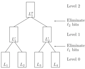
The idea behind our modification (which we call the “extended k-tree algorithm”) is the fol- lowing. We can think of the originalk-tree algorithm aseliminating (i.e., finding vectors that sum to zero on) a fixed number logm bits in each round (except for the last round, where 2 logm bits are eliminated)§. This choice keeps the list length constant over all rounds, thereby balancing the work done in each round. (See section 2 for a more precise description of the k-tree algorithm.) While this guarantees a minimum maximal list length, it also entails the strong requirement (1.2).
In our extension, we vary the number of bits eliminated (and thus the intermediate list lengths) in each round, in such a way that ultimately more bits can be eliminated in total.
To illustrate how this can help, consider again the k = 4 example from earlier, and suppose now that we take a smaller value of m, say m = 22n/7 instead of m = 2n/3. (Note that this value takes us outside the scope of Wagner’s algorithm, but is still within the existence bound (1.1).) If we eliminate ℓ1 = n/7 bits in the first round (instead of n/3 as previously), then E[|L′1|] = 2−n/7|L1||L2|= 23n/7. We then eliminate the remainingℓ2= 6n/7 bits in the second round, giving us an expected number of solutions equal to
2−6n/7E[|L′1|]E[|L′2|] = 2−6n/726n/7 = 1;
§Throughout the paper, log denotes base-2 logarithm unless otherwise stated
thus we again expect the algorithm to find a solution. This gives an algorithm with expected running time ˜O(23n/7) for this particular set of parameters, which is still significantly better than the ˜O(2n/2) na¨ıve algorithm.
The key step in designing our algorithm is to specify an optimal strategy for choosing the expected list lengths (or equivalently, the number of bits to be eliminated) in each round. We do this by formulating this optimization problem as an integer program, which we are then able to solve analytically. Perhaps surprisingly, the optimal strategy turns out to be to let the lists grow in the first few rounds without eliminating any bits, and then to switch to a second phase in which a fixed number of bits are eliminated in each round. The role of the first phase is apparently to simply increase the pool of vectors (by summing combinations from the original lists) until the number of vectors is large enough for the elimination phase to work successfully.
We then go on to address the failure probability of the algorithm. Note that both our algorithm as described above, and Wagner’s original k-tree algorithm, are based only on an analysis of the expected number of solutions found, which says nothing useful about the probability that a solution is actually found. In the last section of the paper, we give the first rigorous bound on this probability.
Our analysis, which uses the second moment method, applies to both Wagner’s algorithm and our extension. The upshot is that, for a wide range of parameters, if one na¨ıvely aims for a single solution in expectation, then the failure probability will be at most slightly larger than 3/4. Moreover, at the cost of a small increase in running time, the failure probability can be reduced substantially.
In the final part of the paper, we present a modification of the algorithm that can be used to solve instances where the lists contain vectors over an arbitrary finite field Fr rather than over F2. In this case the problem is generalized to that of finding a suitable linear combination (with coefficients inF∗
r) of vectors summing to zero. Such an algorithm can be used, for example, to find low-weight codewords in non-binary linear codes, or to compute sparse multiples of polynomials in Fr[X].
1.3 Related work
The basic idea of thek-tree algorithm was apparently rediscovered several times. In 1991, Camion and Patarin [5] constructed ak-tree scheme for breaking knapsack-based hash functions. In 2000, Blum, Kalai and Wasserman [3] devised a similar algorithm to prove a conjecture in learning theory.
In 2002, Wagner [13] published a paper dedicated entirely to thek-tree algorithm, including some extensions and several applications.
In the same year, Chose, Joux and Mitton [6] proposed an algorithm for finding low weight parity checks for a linear feedback shift register. Their algorithm is similar to the 4-tree algorithm.
Unlike the other authors, Choseet al.propose a scheme where the number of eliminated bits varies from round to round. However, their motivation for doing so is quite different from ours, leading to very different results: unlike thek-tree algorithm, their algorithm findsall the solutions, and their choice of parameters is designed so as to minimize the memory use without sacrificing too much speed. Our goal, on the other hand, is to find only a single solution, and we choose the parameters so as to minimize running time (and memory use) for that purpose.
In 2004, Coron and Joux [7] used Wagner’s algorithm to break a hash function based on error correcting codes. Since Wagner’s condition (1.2) does not hold in their case, they tweaked the algorithm by removing one level of the tree and working on lists that were sums of pairs of vectors.
This strategy is a special case of our algorithm, and hence can be viewed as an interesting application of the extendedk-tree algorithm. The attack by Coron and Joux was subsequently refined by Augot,
Sendrier and Finiasz [8] to a variant that does not always eliminate the same number of bits per round.
We are not aware of any previous analysis of the failure probability of the original k-tree algorithm; however, some modified versions have been analyzed, as we now discuss.
First, Blum, Kalai and Wasserman [3] analyzed a related algorithm, which differs from Wagner’s algorithm in that it searches for collisions in a single list. Another difference is that only a subset of the valid pairs is selected in the merging step. In 2005, Lyubashevsky [10] analyzed a variant of Wagner’s algorithm devised to solve the integer subset-sum problem; thus the list elements are integers mod t rather than bitstrings. As in the Blumet al. algorithm, only a subset of the valid pairs is used when merging. In this construction, the length of the lists has to be roughly the square of the length that Wagner’s algorithm prescribes. In 2008, Shallue [12] modified Lyubashevsky’s algorithm so that the merging step selects a larger subset of valid pairs. As a result, in order to achieve non-trivial failure probability the lists need to be of length O(mlogm) where m is the length required by Wagner’s algorithm.
A key difference between all these three constructions and Wagner’s original algorithm is that the list merging step does not select all valid pairs. This has two drawbacks. First, it results in an inflation of the list length (and hence running time) relative to Wagner’s algorithm. Second, in these constructions the merge cannot possibly expand the list length, which is a key ingredient of our extended algorithm.
Finally, we briefly mention an alternative approach to the k-sum problem which is applicable in the regime where k ≥ n (which typically does not hold in the kind of applications mentioned earlier). Bellare and Micciancio [2] show that in this scenario thek-sum problem can be solved by Gaussian elimination in timeO(n3+kn).
2 The extended k -tree algorithm
In this section we present a framework for our extended k-tree algorithm; as we shall see, the originalk-tree algorithm of Wagner [13] is a special case.
Given an instance of thek-sum problem as described in the Introduction, the (extended)k-tree algorithm proceeds in q rounds, wherek = 2q is the number of input lists. In each round, pairs of lists are merged to form a new list, so that the number of lists is halved in each round. For example, in the first round the listsL1andL2are merged into a new listL′1, the listsL3andL4are merged into a list L′2, and so forth. Specifically, the listL′i is composed of all the sums x+y with x∈L2i−1 and y∈L2i such thatx+y is zero on the firstℓ1 bits. The integer ℓ1 is a parameter of the algorithm that is to be selected for optimal performance. We say that the first roundeliminates ℓ1 bits.
The other rounds are akin to the first one. In the second round, lists L′′1, . . . L′′2q−2 are created from L′1, . . . , L′2q−1, eliminating a further sequence of ℓ2 bits and thus causing the vectors in the lists L′′1, . . . , L′′2q−2 to be zero on the firstℓ1+ℓ2 bits.
Iterating this procedure for q rounds, we get a single, final list containing vectors that are zero on the firstPq
i=1ℓi bits, each of which is a sum of the formPk
i=1xi withxi ∈Li. Since our goal is to find sums that are zero on allnbits, the final list will contain sums of the desired form provided
that q
X
i=1
ℓi ≥n. (2.1)
L1 L2 L3 L4
L′1 L′2
L′′1
Eliminate
Eliminate ℓ1 bits ℓ2 bits
Level 0 Level 1 Level 2
Figure 1: Thek-tree algorithm for k= 4.
The algorithm can be visually represented as a complete binary tree of heightq, with each node containing a list of vectors. Leveljof the tree contains the lists afterjrounds of the algorithm, with the leaves (at level 0) containing the input lists L1, . . . , Lk. Figure 1 gives a pictorial illustration of the case k= 4.
Note that, since the input lists are random, the lengths of the lists at all internal nodes within the tree are random variables. We will write Mj for the random variable representing the length of a list at level j. The distribution of Mj is determined by the values ofm and ℓ1, . . . , ℓj.
Note that Mq is the total number of solutions found by the algorithm. We will also specify as a parameter the desired expected number of solutions found, which we write as 2c. So our goal is to ensure that
E[Mq]≥2c. (2.2)
Canonically one may think of the value c = 0, i.e., a single solution is sufficient in expectation.
(This is what we did in the examples in the Introduction.) However, as we will see in section 4, the failure probability of the algorithm can be made significantly smaller by increasing the value of c slightly (e.g., by choosingc= 1). This entails a slight tightening of condition (1.1), which becomes
m≥2(n+c)/2q. (2.3)
In the remainder of the paper we shall always assume that (2.3) holds. We will also assume that
m≤2(n+c)/(q+1), (2.4)
since Wagner’s algorithm applies for all largerm. Finally, for technical reasons we will also assume that c < 2 logm; since typically c is a small constant (such as 0 or 1), while the list lengths are quite large, this represents no restriction in practice.
Note that the choice of the parameters ℓi critically impacts the behavior of the algorithm.
Roughly speaking, increasingℓi has the effect of reducing E[Mj] for every j≥i, while decreasing it has the opposite effect. Since the running time is essentially proportional to the sum of the lengths of the lists at internal nodes in the tree, for optimal performance we seek a strategy for choosing
theℓi such that E[Mj] is not too large for any 1≤j≤q−1; however, we also need to ensure that the constraints (2.1) and (2.2) both hold.
As a simple example, assuming m is a power of two, Wagner’s original k-tree algorithm [13]
choosesℓj = logm forj= 1, . . . , q−1 andℓq = 2 logm, leading to E[Mj] =mfor j= 1, . . . , q−1 and E[Mq] = 1, i.e., all lists (except the last) have the same expected length as the initial lists. In this case, condition (2.1) translates to (q+ 1) logm≥n, which is exactly Wagner’s condition (1.2) discussed earlier. If this condition holds, this choice for the ℓi works very well. One of the main goals of this paper is to find optimal choices for theℓi when (1.2) does not hold.
Remark: The merging step at each node, as presented above, retains pairs of vectors whose sum on certain subsequences of bits is zero. As a result, the algorithm produces only solutions that satisfy these constraints. This is an arbitrary choice that was made only to simplify the presentation. In fact, the target values for the sums at each node could be chosen randomly, subject only to the requirement that the sum of all the target values at any level equals zero. This yields an algorithm that chooses a random solution, rather than one of the above special form.
3 Choosing the parameters
As we saw in section 2, our algorithm is specified by the parametersℓi that determine the number of bits eliminated in each round. Our goal now is to find an optimal choice for theℓi when m,q,n andcare given, i.e., to find a set of parameters that minimizes the running time while guaranteeing 2c solutions in expectation.
In section 3.1, we will show how to reduce the problem of finding the optimal ℓi to an integer program. We will then give an explicit solution to this integer program in section 3.2.
3.1 The integer program
We start by giving a formula for the expected list length at each level of the tree. We write b0 := logm, and define 2bj as the expected length of the lists at level j of the tree. Then we have
bj = 2bj−1−ℓj, (3.1)
where ℓj is the number of bits eliminated at level j. To see this, let the random variable Mj be the number of vectors appearing in the list at some fixed node at level j, so that 2bj = E[Mj].
WritingMj−1l ,Mj−1r for the number of vectors in the lists at the left and right children of the node respectively, we have
2bj = E[Mj−1l Mj−1r ]2−ℓj = E[Mj−1l ]E[Mj−1r ]2−ℓj = 22bj−1−ℓj,
which proves (3.1). Since the list at the root of the tree consists exactly of the solutions found by the algorithm, the expected number of solutions found is 2bq. The maximum expected list length that the algorithm has to process is
0≤j≤q−1max 2bj. (3.2)
(Note thatbq does not appear in this formula; this is because we do not need to explicitly compute the complete list of all matches, but can stop as soon as we have found a solution.) Since the expected running time of our algorithm is ˜O(2q+u), where 2u is the maximum expected list length,
our goal will be to choose theℓj so as to minimize the expression (3.2). For our formulation of the integer program it will be convenient to use both the ℓj and the bj as variables. However, it can be seen from (3.1) that theℓj determine the bj and vice versa.
Suppose now that we specify that the expected number of solutions found by the algorithm should be at least 2c. This leads to the following integer program:
minimizeu
s.t. bj ≤u j= 0, . . . , q−1
ℓj ≥0, ℓj integer j= 1, . . . , q Xq
j=1
ℓj ≥n bq≥c.
Example: For n = 100, m = 216, and q = 4 (which are typical parameter values in, e.g., codeword-finding applications), and setting c = 1 (for an expected two solutions), the integer program dictates that we should choose ℓ1 = 9, ℓ2 = 23, ℓ3 = 23, ℓ4 = 45. This solution has an expected maximum list length of 223, resulting in roughly 223+4= 227 expected vector operations, which is a very feasible computation.
For the same parameters, the na¨ıve algorithm performs approximately 250 operations, which is plainly unreasonable. Wagner’s original algorithm is not intended to be used in this case, but if we use it anyway, eliminating 16 bits in each round to keep the list lengths constant, it will only succeed with probability at most 2−20. Since a single run of Wagner’s algorithm costs roughly 216+4= 220operations in this case, the expected running time (with repeated trials until a solution is found) would be about 240, again prohibitively large.
3.2 Solution of the integer program
We will now compute the optimum of the above integer program. We shall first consider the linear programming relaxation (without the integrality constraint), and then show that its solution can easily be rounded to a solution of the integer version.
We proceed by showing that the optimal solution of the LP has three “phases.” In the first phase, for small i(i.e., low levels of the tree), theℓi are all equal to zero, andbi is doubled (so the length of the lists is squared) in each round. In the second phase, for larger values of i, bi (and hence the length of the lists) remains fixed, meaning that a fixed number of bits ℓi is eliminated in each round. The third phase consists only of the final round, where the list is collapsed to the desired expected number of solutions, which is 2c.
More precisely, we will prove the following.
Theorem 3.1 For any set of parameters n, m, q, c satisfying conditions (2.3), (2.4) and c <
2 logm, the linear program defined above is feasible and has an optimal solution of the following
form:
bi= 2ib0 ℓi= 0, for 1≤i < p;
bp=u ℓp= 2pb0−u;
bi=u ℓi=u, for p < i < q;
bq=c ℓq= 2u−c;
where p is the least integer such that
n≤(q−p+ 1)2plogm−c, and u is given by
u= n+c−2plogm
q−p .
Note that the valuei=p marks the beginning of the second phase.
Proof: We will first show that the linear program is feasible. To this end, setℓ1=· · ·=ℓq−1 = 0, ℓq=n. From (3.1), it follows then thatbi = 2ib0fori < q, andbq = 2qb0−n. Setu= maxi≤q−1bi= 2q−1b0.
We now verify that this solution is feasible. Clearly, all theℓiare non-negative andPq
i=0ℓi≥n.
The condition bq ≥c translates to 2qb0 ≥n+c, which, recalling that b0 = logm, is equivalent to condition (2.3) and hence satisfied by assumption. Thus the solution is feasible.
Next we will show that any solution not of the form given in the statement of the theorem can be strictly improved. Since the LP is bounded (as can readily be checked from (3.1)) this will establish the theorem.
Consider first a feasible solution ~ℓ= (ℓ1, . . . , ℓq) in which there is some indexj∈ {1, . . . , q−1} such thatℓj >0 andbj < u. Then for suitably small ε >0 the transformation
ℓj 7→ℓj −ε, ℓj+1 7→ℓj+1+ 2ε, bj 7→bj+ε (3.3) yields another feasible solution with the same value of u. (This can easily be checked using the recursive definition (3.1).) Note that this transformation increases the sum of the ℓi by ε, so the constraint Pq
i=1ℓi ≥nbecomes slack.
Similarly, in a feasible solution ~ℓin which bq> c, the transformation
ℓq 7→ℓq+ε, bq7→bq−ε (3.4)
yields another feasible solution with the same value ofu and makes the sum constraint slack.
Thus any solution that does not satisfy the conditionsℓj = 0 orbj =ufor allj∈ {1, . . . , q−1}, andbq =c, can be transformed into a solution with the same value of the objective functionuthat does satisfy these conditions and where in addition Pq
i=1ℓi > n.
We now show that such a solution can be transformed into one with a smaller value of u. Since u = maxjbj, it is enough to show that any maximal bj can be reduced; the procedure can be repeated if necessary. We argue first that we cannot haveb0 = maxjbj. For if so, substituting the recursion (3.1) intoP
iℓi > n, we getPq
i=1(2bi−1−bi)> n, or equivalently 2b0+Pq−1
i=1 bi−bq> n,
and hence (q+ 1)b0−c > n; but this violates condition (2.4). So now let 1≤j ≤q−1 be an index such thatbj =u, and consider the transformation
ℓj 7→ℓj+ε, ℓj+17→ℓj+1−2ε, bj 7→bj−ε. (3.5) We claim that, for small enoughε >0, this yields a feasible solution. To see this, we just need to check that ℓj+1 >0. But if ℓj+1 = 0 then by (3.1) we would have bj+1 = 2bj = 2u. Ifj+ 1 < q this gives a contradiction because bj+1 ≤u. And if j+ 1 =q then c=bj+1 = 2u≥2b0 = 2 logm, which violates our assumption that c <2 logm.
The above argument shows that any optimal solution must satisfy ℓj = 0 orbj =u for 1≤j≤ q−1. We need to verify that the indices j for which ℓj = 0 form an initial segment. To see this, simply observe that if bj = u and ℓj+1 = 0 then from (3.1) we have bj+1 = 2u which contradicts the constraintbj+1≤u.
Equation (3.1) can now be used to reconstruct the values of ℓp, . . . , ℓq, b1, . . . , bp−1 by direct computation.
It remains to determinepandu. Frombp−1 ≤uand 0≤ℓp= 2pb0−uwe get 2p−1b0 ≤u≤2pb0. Since, as we have seen above, the constraint P
iℓi ≥ n must be tight in an optimal solution, we also haven=Pq
i=1ℓi = (q−p)u+ 2pb0−c. Substituting the above bounds onu into this equation forngives
n∈[(q−p+ 2)2p−1b0−c,(q−p+ 1)2pb0−c].
Note that for distinct p ∈ {1, . . . , q−1} the interiors of these intervals are disjoint, and that the intervals cover [(q + 1)b0 −c,2qb0−c], which is precisely the range of values of n for which the algorithm is applicable. So for given n, m, q and c satisfying (2.3) and (2.4), there is a unique choice of p (except at the endpoints, which belong to two intervals; either choice of p yields the same solution in this case). Oncepis known, we can solve forufromn= (q−p)u+ 2pb0−c.
The optimal solution to the linear program as given by Theorem 3.1 can result in fractional values for the ℓi; however, we need them to be integers. Fortunately, it turns out that the optimal solution of the corresponding integer program can be obtained by a simple rounding of the LP solution. This is the content of the following claim.
Claim 3.2 Assume b0 and c are integers. The optimal solution ℓ1, . . . , ℓq of the integer program can be obtained by replacing u by⌈u⌉ in the LP solution of Theorem 3.1.
Note that the value ofp is not changed by this rounding operation.
Proof: Clearly, if this solution is feasible then it must be optimal since⌈u⌉is the smallest integer exceeding u. Write ˜u,ℓ˜1, . . . ,ℓ˜q,˜b1, . . . ,˜bq for the putative integer solution obtained by applying the above rounding to the LP solution u, ℓ1, . . . , ℓq, b1, . . . , bq.Then Pq
i=1ℓi = (q−p)u+ 2pb0−c, which is increasing with u since q−p ≥ 0; hence Pq
i=1ℓ˜i ≥ n, as required. To see that ˜ℓj ≥ 0, note that clearly ˜ℓj ≥ℓj for allj exceptj=p. But we also have ˜ℓp ≥0 because z−u≥0 implies z− ⌈u⌉ ≥0 for any integer z.
Finally, it can be checked by direct computation that the ˜bi and ˜ℓi still satisfy (3.1).
Remark: The constraint P
iℓi ≥ n may not be tight in the given integer solution. This is not a problem however; for example, the length of the vectors can be increased to P
iℓi by padding them with random bits at the end. Any solution to this new instance will also be a solution to the original one.
Note that the value of u given in Theorem 3.1 does not change if we replace n by n+c and c by 0. So for simplicity we will assume c= 0 for the remainder of this section, i.e., we will assume that the algorithm aims for just one solution in expectation.
Corollary 3.3 For all parameters n, m, q such that 2n/2q ≤ m ≤ 2n/(q+1), the expected running time of the algorithm is O(2˜ q+u∗(n,m,q)), where u∗(n, m, q) is the optimal value of u in the LP for parameters n, m and q as given in Theorem 3.1.
Moreover u∗(n, m, q) is a continuous, convex, piecewise affine and decreasing function of logm.
Proof: Up to logarithmic factors, the running time is equal to the sum of all the list lengths that the algorithm processes. There are 2q+1 −1 = O(2q) lists, each of expected length at most 2⌈u∗(n,m,q)⌉=O(2u∗) by Claim 3.2, resulting in an expected running time ˜O(2q+u∗(n,m,q)).
By Theorem 3.1, p is piecewise constant (as a function of n, m, q), and hence u∗(n, m, q) is piecewise affine as a function of logm. The other properties are easy to verify.
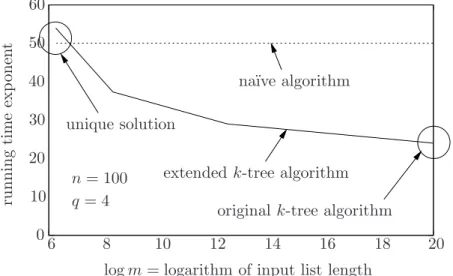
To illustrate this Corollary, consider the plot in Figure 2 which compares the expected running time exponents of the na¨ıve algorithm and the extended k-tree algorithm. We take the same example as in section 3.1, with q = 4, n= 100. The relevant range form is then 26.25 ≤m≤220. At the very right, for m = 220, our algorithm is the same as the original k-tree algorithm, and uses roughly 220+4 = 224vector operations. As noted before, the originalk-tree algorithm does not work form <220 in this setting.
unique solution
na¨ıve algorithm
extended k-tree algorithm original k-tree algorithm
logm= logarithm of input list length n= 100
q= 4
6 8
10
10 12 14 16 18
20
0 20 30 40 50 60
runningtimeexponent
Figure 2: Comparison of the extendedk-tree algorithm with the na¨ıve algorithm
At the left border, for m = 26.25, our algorithm is nothing but a (somewhat complicated) variant of the na¨ıve algorithm, and the estimated expected running time is 250+4. For m <26.25 the probability that any solution exists at all decays rapidly.
Note that our algorithm contains both the na¨ıve algorithm and the originalk-tree algorithm as special cases, but does substantially better than the na¨ıve algorithm for a wide range of values of m where the originalk-tree algorithm no longer works.
Remark: In the graph we are seemingly overtaken by the na¨ıve algorithm shortly beforem= 26.25. This is just an artifact of our analysis. While our running time estimate is the best that can be achieved purely in terms of the maximum list length, it should be noted that the additional factor 2q of Corollary 3.3 is crude for smallm, because (as can be seen from the LP solution) in that case only very few lists will have maximal length. Since for m = 26.25 our algorithm is essentially the same as the na¨ıve algorithm, it must in fact have the same complexity.
4 Analysis of the failure probability
Up to this point, we have implicitly assumed that it is enough to design the algorithm so that the expected number of solutions found is at least one, and that a single run of the algorithm would then yield a solution with good probability. The goal of this section is to justify this assumption, i.e., to show that the number of solutions per run is concentrated around its expectation in most interesting cases, and that therefore the algorithm does indeed produce an output with reasonable probability. We note that our analysis applies also to the originalk-tree algorithm of Wagner [13], whose failure probability had apparently not previously been bounded.
4.1 Preliminaries
Let N be the number of solutions found by the algorithm. Thus the algorithm succeeds when N > 0 and fails if N = 0. Write the input lists as L1 = (x11, . . . , x1m), . . . , L2q = (x21q, . . . , x2mq).
Let S ={1, . . . , m}2q, and let a= (a1, . . . , a2q) ∈ S. Then the vector of indices a corresponds to a solution found by the algorithm if x1a1 +· · ·+x2aq
2q = 0, and if in addition the xiai satisfy the constraints imposed by the internal nodes of the tree. For example, we must havex1a1+x2a2 = 0 on the firstℓ1 bits, and so on; there are 2q−1 such constraints to be satisfied.
If we write Ia as the indicator random variable of the event that a is a solution, then N = P
a∈SIa.Writing µ:= E[Ia], we get by Chebyshev’s inequality that Pr(N = 0)≤ Var(N)
E[N]2 ≤ |S|µ+P
a,b∈S,a6=bCov(Ia, Ib)
|S|2µ2
≤E[N]−1+ Eab[Cov(Ia, Ib)|a6=b]
µ2 , (4.1)
where Eab[·] denotes expectation over a and b chosen independently and uniformly at random from S.
IfIaandIb were independent whenevera6=b, then this probability would of course be bounded by E[N]−1. However, Ia and Ib can be highly correlated if a and b have many components in common. We therefore have to bound the covariance terms in (4.1).
4.2 Incidence trees
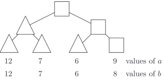
Fix a, b∈ S. The incidence tree for a and b is a complete binary tree of height q with the nodes being either squares () or triangles (△) according to the following rules. Theith leaf (from the left) is associated with the ith components of a and b. A node is a triangle if and only if all the components ofa and b in the leaves below it are equal. Note that the shape of any internal node
12
12 7
7
6
6 9
8
values ofa values ofb
Figure 3: The incidence tree of a= (12,7,6,9) and b= (12,7,6,8).
can be deduced from the shape of its children: it is a triangle if and only if both its children are triangles. For an example of an incidence tree withq = 2, see Figure 3.
If the incidence tree of aand b is known, then the value of Cov(Ia, Ib) can be computed easily.
First note that we can factor Ia as follows:
Ia=Y
y
Ja(y),
where y runs over all the internal nodes of the tree, andJa(y) is the indicator random variable of the event that the constraint implied by node y is satisfied by a. (Note that the constraint at y involves onlyℓj bits, wherejis the level ofy; this constraint can be satisfied even if the constraints at some of the descendants ofy are not.)
For fixed internal nodesy and z, the random variables Ja(y) andJb(z) are equal ify=zandy is a triangle in the (a, b)-incidence tree. OtherwiseJa(y) andJb(z) are independent. In particular, the Ja(y) (where y runs over the internal nodes) are mutually independent. So for any internal node y, we have
E[Ja(y)Jb(y)] =
(E[Ja(y)] = 2−ℓlevel(y) ify is a triangle;
E[Ja(y)]E[Jb(y)] = 2−2ℓlevel(y) ify is a square.
Here, level(y) denotes the level of the node y in question. Writing Fab := EQ
ysquareJb(y)
= 2−Pysquareℓlevel(y), we have
E[IaIb] = E[Ia Y
ysquare
Jb(y)] = E[Ia]E[ Y
ysquare
Jb(y)] =µFab. We can then compute the covariance Cov(Ia, Ib) as follows:
Cov(Ia, Ib) = E[IaIb]−µ2=µ(Fab−µ). (4.2) 4.3 Computing the expected covariance
We now derive an exact recursive formula for Eab[Cov(Ia, Ib)|a 6= b]. To this end, we study the behavior of the random variableFab when aand bare random. For a nodey at level j≥1, define
Sj := Y
za square descendant ofy
2−ℓlevel(z),
wherezruns over all square internal nodes in the subtree whose root isy. With this notation, note thatFab =Sq. Forj ≥1, we write Eab[Sj] for the expectation (over a, b) ofSj, conditional on the node with respect to which Sj is defined being a square. Then, settingS0 = 1, we have
Eab[Sj] = 2−ℓjEab[Sj−1] Eab[Sj−1](1−αj)+αj
, (4.3)
where
αj := Pr(a level-j node y has a △child|y is a) = 2·m−2j−1
1 +m−2j−1. (4.4) Now, equation (4.3) can be used recursively to compute Eab[Sq]. From this we can compute Eab[Cov(Ia, Ib)|a6=b] =µ(Eab[Sq]−µ), which follows from (4.2) and the facts that Fab =Sq and Eab[Sq] = Eab[Sq|a6=b].
Putting everything together, we get that the error bound (4.1) of section 4.1 can be written as Pr(N = 0)≤E[N]−1+µ−1Eab[Sq]−1, (4.5) where Eab[Sq] is the solution to the recurrence (4.3). Note that the quantityµ−1Eab[Sq]−1 captures the contribution due to dependencies between the indicator random variablesIa.
Remark: Inequality (4.5) provides a method for numerically bounding the failure probability of the extended k-tree algorithm for any choice of the parameter values (ℓ1, . . . , ℓq), provided only thatP
iℓi ≥n. Of course, the values N and Eab[Sq] will depend on the choice of theℓi.
Example: Consider our running example withq = 4,m= 216,n= 100,ℓ1= 9, ℓ2 = 23,ℓ3 = 23, ℓ4 = 45. With these settings we get two solutions per run in expectation (c= 1); hence we would like the failure probability to be close to 1/2 (as would be the case if the random variables Ia were independent). Using the above recursive method to compute Eab[Cov(Ia, Ib) | a 6= b], we get a bound on the failure probability of 0.5000017. Thus the effect of dependencies is very small, as desired.
4.4 Bounding the failure probability
In this section we consider the optimal choice of the parameters ℓi, as described in section 3. For this choice of theℓi, we provide the followinganalytic upper bound on the failure probability that is useful in many applications.
Theorem 4.1 If ℓ1, . . . , ℓq are chosen optimally as in section 3.2, then the algorithm will fail to find a solution with probability at most
2−c+ exp(qk/m)−1, where 2c = E[N]is the expected number of solutions.
Proof: In light of inequality (4.5), it is enough to show that the quantity µ−1Eab[Sq] is bounded above by exp(qk/m).
Define sj := Eab[Sj]. From (4.3), we have sj = 2−ℓjs2j−1 1−αj+sαj
j−1
withs0 = 1. Let µj :=
2−ℓjµ2j−1 with µ0 = 1. Note that µj is the probability that a fixed partial sum appears in a node at level j; in particular µ=µq. By inspecting the recursions, we also get µ =µq = 2−Pqi=1ℓi2q−i, and µj ≤sj.
We also definetj :=m−2j and remark that t−1j is equal to the number of partial sums that are candidates to appear in a node at levelj; hence the expected list length at levelj is equal tot−1j µj. Note also from the definition (4.4) of αj that αj ≤2tj−1.
Unwinding the formula forsq, we get sq= 2−Pqi=1ℓi2q−i
q−1Y
j=0
1−αj+1+ αj+1 sj
2q−j−1
≤µ·
q−1Y
j=0
1 +2tj
µj
2q−j−1
=µ·exp
Xq−1
j=0
2q−j−1ln
1 +2tj
µj
.
Now we bound the sum in the exponent. Noting that ln(1 +x) ≤ x, and that tjµ−1j = 2−bj, the summand inj can be bounded above by 2q−j−bj. Sincebj is increasing inj(for the optimal choice of ℓj given by Theorem 3.1 and Claim 3.2), the largest summand is the one for which j = 0, so estimating the sum by takingq times the largest summand we get
µ−1Eab[Sq] =µ−1sq≤exp(q2q/2b0) = exp(qk/m), which completes the proof.
To interpret Theorem 4.1, note that the additional error probability due to dependencies is approximately qk/m, assuming this quantity is fairly small. Hence ifc= 1, we will get an overall error probability very close to 1/2 providedqkis much smaller thanm. This condition is satisfied in particular for the various applications mentioned in the introduction. E.g., for our running example above withn= 100,m= 216,q= 4,c= 1, Theorem 4.1 bounds the failure probability by 0.50097, which is very close to 1/2 (the best we can hope for from a second moment analysis), and only slightly larger than the value 0.5000017 computed at the end of the previous subsection.
Note also that in typical applications (when qk/m is small) the principal variable controlling the error probability isc; ifcis not too large, increasingccauses the failure probability to decrease significantly.
Remark: The failure probability given by Theorem 4.1 differs at first sight qualitatively from those in [10, 12] for the special case of Wagner’s algorithm in that it does not decay to zero with the list length. However, our bound applies to the optimal algorithm for given n,m,q andc, while in [10, 12] the list lengthmis required to be larger by a factor ofαin order to achieve the bound on the failure probability (which decays exponentially withα). Obviously, since we achieve a constant failure probability for the given list length m, increasing the list length by a factor of α would allow us to runα independent trials of our algorithm, which also causes the failure probability to decrease exponentially with α.
To obtain a nontrivial failure probability with Theorem 4.1, it is necessary to aim for more than one solution in expectation (c > 0). We will now show that even if we aim for one solution, or indeed somewhat less, the failure probability can still be usefully bounded in many cases.
Corollary 4.2 If ℓ1, . . . , ℓq are chosen optimally as in section 3.2 with−2 logm+ 1< c≤0, then the algorithm will fail to find a solution with probability at most
1−2c−1 3
2 −exp(qk/m)
.
Proof: Consider an instanceI with parametersn, m, q. We wish to bound the failure probability of the algorithm when solving I with c ≤ 0. From the instance I, build a new instance I′ with parameters n+c−1, m, q by removing the last 1−c bits from each vector in every list. (By our assumed lower bound on c, these bits are all eliminated in the last round.) The choice of the ℓi made by the algorithm for instance I′ withc= 1 is the same as that for instanceI with the given value of c. If the algorithm is applied to I′, by Theorem 4.1 it finds a solution with probability at least
3
2 −exp(qk/m).
If we now consider the corresponding sum in I, we get a vector that has a zero in all positions except possibly for the last 1−c of them. The values in these positions will all be zero with probability 2c−1; in that case, this solution will also be found by the algorithm when it runs on instance I with the given value of c. Therefore the algorithm fails on I with probability at most 1−2c−1 32 −exp(qk/m)
,as claimed.
5 Larger alphabets
Thek-sum problem has a natural generalization to non-binary alphabets, where the goal is now to find a non-trivial linear combination of vectors summing to zero. Formally, we state the problem as follows.
Let r be a prime power. We are given k = 2q lists L1, . . . , Lk, each of length m, containing (independent, uniformly sampled) random vectors from Fnr. We wish to find x1 ∈L1, . . . , xk∈Lk and λ1, . . . , λk ∈F∗r such that
λ1x1+· · ·+λkxk = 0.
The requirement thatall theλihave to be nonzero is arguably somewhat artificial, since for typical applications any solution with not all theλi zero is satisfactory. However, this formulation has the advantage that it does indeed generalize the binary case. Moreover in both the binary and the non- binary cases, a solution allowing some of theλi to be zero can be sought by adding the zero-vector to every list.
The k-sum problem over non-binary alphabets can be used to solve general finite-field versions of the various problems mentioned in the introduction. For example, it can be used to find low- weight codewords in codes with comparatively few redundant symbols defined over a moderate size alphabet, such as the erasure-correcting codes analyzed in [4]. Typical parameter values that might arise in such a setting are the following, which we shall use as our running example throughout this section:
Example: We work in F64, and consider vectors of n = 18 symbols; such a vector is then representable with 108 bits. We wish to find a sum of k= 8 of them from 8 lists, such that their sum equals zero.
The obvious generalization of thek-tree algorithm consists of just putting every possible nonzero scalar multiple of every vector into the lists. This has two serious drawbacks, however. First, it inflates the list lengths (and hence both the space and time requirements) by a factor of r−1;
and second, it destroys the independence of the vectors in a list, making analysis much harder. In the following, we develop an alternative version of the extended k-tree algorithm tailored to the non-binary case. Our version suffers at most only a factor 4 increase in space and a factor √
r increase in time compared to the binary version with the same parameter values. Moreover, we are still able to carry out a full analysis of our algorithm, including the failure probability, similar to that for the binary case given earlier. The algorithm works for a range ofm analogous to that for the binary case (see (5.3) below).
5.1 The merging procedure
The starting point for our modified algorithm is a more involved merging procedure, which ensures that only a single scalar multiple of each relevant linear combination is retained in the lists at each stage of the algorithm. This is key to avoiding a blow-up of a factor r−1 in the list lengths. In this section we describe this merging procedure.
We are given two listsL1,L2 and an integerℓdesignating the number of positions to eliminate.
We wish to construct a minimal merged listL, i.e., a list of vectors having the following properties:
• Validity. Every vector inL is of the form λ1x1+λ2x2 withλi ∈F∗r andxi∈Li and it has a prefix ofℓ zeros.
• Completeness. If λ1, λ2 ∈ F∗
r, x1 ∈ L1 and x2 ∈ L2 are such that y = λ1x1 +λ2x2 has ℓ leading zeros, then there exists a µ∈F∗r such that µyappears in L.
• Minimality. Ify=λ1x1+λ2x2appears inL, then no other linear combinationµy= (µλ1)x1+ (µλ2)x2 with µ 6= 1 appears in L. (A scalar multiple of y may of course appear in L by coincidence, i.e., if it can be written as a linear combination that is not just a scaling of λ1x1+λ2x2.)
Such a list can be efficiently computed as follows. By multiplying the vectors in the lists with suitable constants, we can assume they are all of thenormalized form
(0, . . . ,0,1,∗, . . . ,∗); (5.1) that is, the leftmost nonzero position, if it exists, is a 1.
Let x1 ∈ L1 and x2 ∈L2 be two normalized vectors in their respective lists, and let ℓ be the number of positions that we wish to eliminate. We make the following observations:
1. If eitherx1orx2 has less thanℓleading zeros, then the only possible valid linear combinations λ1x1+λ2x2 with ℓ leading zeros satisfyλ1+λ2 = 0. In particular the first ℓ symbols of x1 and x2 are equal in this case.
2. Otherwise, bothx1 andx2 have at leastℓleading zeros. Then there are exactlyr−1 distinct valid sums of x1 and x2 which have at least ℓ leading zeros, namely all sums of the form x1+λx2,where λruns overF∗
r.