Bed topography and subglacial landforms in the onset region of the Northeast Greenland Ice Stream

(1)

Cite this article:Franke S, Jansen D, Binder T, Dörr N, Helm V, Paden J, Steinhage D, Eisen O (2020). Bed topography and subglacial landforms in the onset region of the Northeast Greenland Ice Stream.Annals of Glaciology61 (81), 143–153. https://doi.org/10.1017/

aog.2020.12

Received: 3 October 2019 Revised: 26 February 2020 Accepted: 27 February 2020 First published online: 18 March 2020 Key words:

Glacial geomorphology; glacier flow;

ice streams; processes and landforms of glacial erosion; radio-echo sounding Author for correspondence:

Steven Franke, E-mail:steven.franke@awi.de

creativecommons.org/licenses/by/4.0/), which permits unrestricted re-use, distribution, and reproduction in any medium, provided the original work is properly cited.

cambridge.org/aog

1Alfred Wegener Institute, Helmholtz Centre for Polar and Marine Research, Bremerhaven, Germany;²Center for Remote Sensing of Ice Sheets (CReSIS), University of Kansas, Lawrence, KS, USA and and³Department of Geosciences, University of Bremen, Bremen, Germany

Abstract

The Northeast Greenland Ice Stream (NEGIS) is an important dynamic component for the total mass balance of the Greenland ice sheet, as it reaches up to the central divide and drains 12% of the ice sheet. The geometric boundary conditions and in particular the nature of the subglacial bed of the NEGIS are essential to understand its ice flow dynamics. We present a record of more than 8000 km of radar survey lines of multi-channel, ultra-wideband radio echo sounding data covering an area of 24 000 km², centered on the drill site for the East Greenland Ice-core Project (EGRIP), in the upper part of the NEGIS catchment. Our data yield a new detailed model of ice-thickness distribution and basal topography in the region. The enhanced resolution of our bed topography model shows features which we interpret to be caused by erosional activity, potentially over several glacial–interglacial cycles. Off-nadir reflections from the ice–bed interface in the center of the ice stream indicate a streamlined bed with elongated subglacial landforms. Our new bed topography model will help to improve the basal boundary conditions of NEGIS prescribed for ice flow models and thus foster an improved understanding of the ice- dynamic setting.

Introduction

The Greenland ice sheet (GrIS) is the second largest land ice mass on Earth and one of the largest contributors to global sea-level rise (Rignot and others, 2011; Gardner and others, 2013; Khan and others, 2014). Observations indicate that its contribution increased from 0.09 mm a⁻¹ for the period 1992–2001 to 0.68 mm a⁻¹for 2012–2016 (IPCC,2019, Section 4.2.2). Apart from a negative surface mass balance due to melting, this contribution to sea level rise is driven by speed-up and retreat of marine-terminating glaciers, leading to ice thin- ning (Howat and others, 2007; Rignot and others, 2011; Gillet-Chaulet and others, 2012;

IPCC,2019). Of particular importance for sea-level predictions are observations of ice streams that transport ice from the interior of the ice sheet to the margin, where it either melts or calves into icebergs. Dynamic processes of ice sheets in Greenland and Antarctica have been progressively included in numerical models to project sea-level changes (Robinson and others, 2012; Church and others, 2013; Goelzer and others, 2020; Rückamp and others, 2020). To simulate present ice stream flow and determine its contribution to the mass balance of ice sheets, we have to understand the natural variability of ice stream dynamics on time scales of tens to thousands of years (Robel and others,2013). For an accurate assessment of the dynamic component of mass loss, ice-sheet flow requires high-resolution observations of the kinematic properties and the geometry conditions.

Ice stream characteristics vary in their geographical settings and thus boundary conditions, for instance ice thickness, subglacial topography, resistive properties of the underlying substrate, subglacial hydrology, as well as atmospheric and oceanic forcing (Robel and others, 2013; Khan and others,2014b; Aschwanden and others,2016). In contrast to flow of outlet glaciers, which often drain ice through bedrock channels or valleys, the high flow velocities of ice streams extend further into the interior of the ice sheet. In some cases their location is not controlled by the bed topography and their boundaries are characterized by narrow shear zones (Truffer and Echelmeyer, 2003). Basal properties of ice streams in Greenland have been mostly investigated at the (now sub-marine) ice-sheet margins of paleo glacier beds with multi-beam bathymetry and marine sediment cores (e.g. Dowdeswell and others, 2014; Hogan and others, 2016; Newton and others, 2017). The beds of paleo ice streams can be hard or soft and often show a large number of streamlined bedforms, mostly parallel to ice flow (Roberts and others,2010). Streamlined bedforms underneath contemporary ice streams in Antarctica have been analyzed by King and others (2009) and Bingham and others (2017) and classified as mega-scale glacial lineations (MSGL) (Stokes and Clark,2002). As subglacial structures may have formed over multiple glaciations, their interpretation is often challenging (Roberts and Long,2005). Little is known about the current conditions of ice stream beds in the central regions of the GrIS, at the onset of streaming ice flow, because data acquisition as well as determination of the geometry and composition of the bed is

(2)

much more difficult to elaborate than on the continental shelf.

For central Greenland it was generally assumed until recently that the ice sheet is underlain by lithified sediment or a crystalline basement. However, a detailed study of Christianson and others (2014) identifies deformable and water saturated sediment several meters thick at the onset zone of the Northeast Greenland Ice Stream (NEGIS), which indicates that deformation of the basal substrate could influence sliding at the ice–bed interface and probably also limit subglacial erosion. Furthermore, Jezek and others (2011) detect elongated landforms probably formed by erosion at the base of the southern flank of the Jakobshavn Ice Stream. Both interpretations indicate a more complex interplay of basal conditions and ice dynamics than present in the case of a simply hard-based ice sheet in Greenland’s interior.

The NEGIS is one of the most prominent features of the GrIS.

With a length of ∼600 km it drains ∼12% of the GrIS via fast-flowing marine-terminating glaciers (Rignot and Mouginot, 2012). Surface ice flow velocities vary from 10 m a⁻¹ at the onset to more than 2000 m a⁻¹at the grounding line of the outlet glaciers (Mouginot and others,2017). The NEGIS differs from all other marine-terminating glaciers in Greenland with its catchment of fast streaming ice flow almost reaching the central ice divide (Joughin and others, 2018). This configuration provides a possible mechanism to transmit forcing from the marine area far inland (Christianson and others, 2014) and several studies have assessed potential changes in the stability of the NEGIS and the ice dynamics in Northeast Greenland (Fahnestock and others, 2001; Joughin and others, 2010; Bamber and others, 2013; Khan and others,2014).

To fully understand the dominating processes and basal boundary conditions driving NEGIS ice flow, in particular in its onset region, on-site measurements are most useful. So far, geophysical surveys investigating the upstream part of the NEGIS concentrated on the immediate surroundings of the East Greenland Ice-core Project (EGRIP) drill site (Fig. 1b), where the ice stream widens (Keisling and others, 2014; Vallelonga and others,2014). High basal melt rates caused by higher continental geothermal heat flux close to the ice divide, as a remnant of the passing of the Icelandic hot spot, are assumed to cause the onset of the ice stream (Fahnestock and others,2001; Rogozhina and others,2016; Martos and others,2018). Further downstream, acceleration is likely caused by subglacial water routing and the presence of high porosity, water-saturated deformable subglacial till, which lubricates the ice stream (Christianson and others, 2014). The geophysical data of Christianson and others (2014) suggest that subglacial till is distributed in the center of our survey region, across the entire ice stream, and is dilatant in the fast-flowing part of the ice stream. The source and routing of till is not yet fully understood. The presence of unconsolidated sediment inside and outside of the NEGIS suggest that sediments are funneled into the NEGIS from the upstream catchment (Christianson and others,2014). Overall, it is difficult to assess which processes dominate the different regions of the ice stream and how they interact (Schlegel and others,2015).

The most important factors controlling ice streams are their basal properties, ice thickness and bed topography, especially as studies of subglacial hydrology are dependent upon bed and surface slope and thus the variation in ice thickness on a local to regional scale (Wright and others, 2008). Without a sufficient spatial data coverage also at the onset of ice streams, it is not possible to assess the nature of the ice stream bed and its properties.

Over the last five decades, most radio-echo sounding campaigns have concentrated on ice divides, domes or fast-flowing outlet glaciers (Bamber and others, 2013; Fretwell and others, 2013). To date, several bed elevation models for Greenland exist (e.g.

Bamber and others, 2013; Morlighem and others, 2017) with

variable resolution and data coverage. Furthermore, modeling studies reveal that an interpretation of isochrones of ice streams is challenging without a detailed knowledge of the bed topography (Leysinger Vieli and others, 2007). These existing limita- tions motivated the acquisition of new high-resolution ice thickness data to improve available bed topographies around NEGIS, in order to help interpret basal structures and thereby determine ice–substrate interaction within NEGIS and in its vicinity (Keisling and others,2014; Vallelonga and others,2014).

In this paper, we use airborne radio-echo sounding data to extend previous geophysical surveys of ice thickness and internal layering around the EGRIP drill site. We provide a new high-resolution bed topography map and discuss the overall gla- ciological setting in the context of NEGIS’ ice dynamics.

Furthermore, we interpret radar returns from subglacial structures, which are not visible in our bed topography DEM, to deduce bed properties and complement simple interpretations based on ice thickness only.

Data and Methods Survey area

The radar data were recorded in the vicinity of the EGRIP drill site in May 2018. A total area of ∼24 000 km² was mapped with 8233 km of profiles sub-parallel and perpendicular to the ice flow direction (Fig. 1b). The central part of the survey area, in direct vicinity to the EGRIP drill site, was covered with a profile spacing of 5 km, further up- and downstream the spacing is 10 km. The area reaches from 150 km upstream to 150 km downstream of the EGRIP drilling site and covers, both, shear margins and parts of the slow-flowing areas outside and adjacent to the ice stream. The shear margins, as boundaries of the ice stream, are mapped over a distance of more than 250 km. The survey lines also cover the transition zone of two northwestern shear margins, located southwest of the EGRIP drill site. Several profiles follow flow paths of a point on the ice surface that has passed through the shear margin.

Radar system

Since 2016 the Alfred Wegener Institute, Helmholtz Centre for Polar and Marine Research (AWI) has been operating a multichannel ultra-wideband (UWB) airborne radar sounder and imager for sounding ice thickness and imaging internal layering and the basal interface of polar ice sheets. The Multichannel Coherent Radar Depth Sounder (MCoRDS) was developed at the Center for Remote Sensing of Ice Sheets (CReSIS) at the University of Kansas in 1993 and has been continuously improved (Gogineni and others,2001; Shi and others,2010). This radar system is designed to operate with multiple antenna elements to increase the power radiated to the target and to compensate for unwanted signals from side echoes and surface clutter by multi-looking and steering a beam to a desired orientation. A comprehensive description of AWI’s UWB radar system is given by Hale and others (2016), Rodriguez-Morales and others (2014) and Wang and others (2014). Its full capabilities were demonstrated by Kjær and others (2018). The radar system is installed on the fuselage of the AWI Polar6Basler BT-67 aircraft and comprises eight transmit channels to transmit and receive radar signals, with a high power transmit and receiver module with fast switching speed. All antenna elements were oriented in along-track (HH) polarization.

The radar system is able to alternate between different pulse duration stages and different receiver gains for each stage to increase the dynamic range. GPS data were acquired by four geodetic NovAtel DL-V3 GNSS receivers operating at 20 Hz. After

(3)

processing we achieve a positioning accuracy of 3–4 cm in horizontal space and 10 cm in elevation for the aircraft.

Data acquisition

Signals were transferred in three stages with different pulse dura- tions and gains (see Table I). The transmitted waveforms are amplitude-tapered with a Tukey window with a taper ratio of 0.08 to reduce range sidelobes caused by the sudden transitions of the envelope in a standard chirped pulse without losing much transmit power (Li and others, 2013). To reduce the data rate and writing speed and to increase signal to noise ratio (SNR), coherent integrations (presums) with zero-pi modulation (Allen and others, 2005) are performed for each waveform depending on the acquisition mode. The aircraft altitude on all survey flights was∼365 m above ground level and the data were acquired at a pulse repetition frequency of 10 kHz. With an aircraft speed of

∼260 km h⁻¹this results in an initial horizontal transmitting inter- val of about 0.7 cm. All profiles were recorded in our narrow band (NB) mode with a frequency range of 180–210 MHz.

Data processing

For data processing, we use the CReSIS Toolbox algorithms for all three spatial domains: vertical range (pulse compression), along- track (fk migration) and cross track (array processing) (see CReSIS-Toolbox, 2019). Further detailed description of the radar data processing is given in the Appendix.

Surface and bed detection

Radar data are recorded in the time domain in two-way travel time (TWT). To convert from radar time to depth, we use the

same relative dielectric constant of 3.15 for depth-conversion as used for synthetic aperture radar (SAR) processing. No compensation was done for a firn layer because the spatial variability of firn properties in dynamic regimes can vary on a scale of a few kilometers (Dutrieux and others,2013). The detection of the ice surface is performed automatically by applying a threshold filter searching for the first maximum in a given time window. This window depends on the flight altitude of the aircraft over ground.

The location of the surface reflection has been verified using the seismic processing and interpretation software Paradigm by Emerson E&P.

At several locations, the range detection of the bed reflector was not clear. Off-nadir reflections offered multiple horizons for bed picks in regions with rough bed topography, where scattered off-nadir reflections and the nadir bed are simultaneously

Fig. 1.(a) Surface velocity map of the Greenland ice sheet, highlighting the NEGIS and its marine-terminating outlets (79NG, Zachariae Isbrae (ZI) and Storstrømmen Glacier (SG)). The survey area (b) is marked with a white outline. (b) Ice flow velocity field of the survey area. The schematic outline of the shear margin was derived from Landsat images. Both maps are displayed in WGS 84/NSIDC Sea Ice Polar Stereographic North (EPSG:3413) and show velocity data of Joughin and others (2018).

Table 1.Acquisition parameters of AWI’s UWB radar campaign in Greenland 2018

Parameter Value

Radar system MCoRDS5

Frequency range^a 180–210 MHz

Waveform signal 1μs, 3μs, 10μs chirp

Waveform presums^b 2, 4, 32

Pulse repetition frequency 10 kHz

Sampling frequency 1600 MHz

Tukey window taper ratio 0.08

Transmit channels 8

Receiving channels 8

Aircraft altitude ∼360 m

Aircraft velocity ∼260 km h⁻¹

aFrequency range from 180 to 210 MHz is referred to narrow band mode (NB).

bPresums are set for each waveform individually.

(4)

present. In most cases, we selected the strongest reflection, because the nadir return signal is usually stronger than off-nadir scattered signals. However, this was not always the case, especially in the areas of strong internal deformation, where englacial layers of high reflectivity reduce the energy and mask the bed return.

Nested bed topography model

We computed an ice thickness and bed elevation model based on our observed ice thickness. We integrate them into the existing dataset of Morlighem and others (2017), BedMachine v3 (BMv3), in order to get a better overview of the regional topographic setting. We create a buffer of 5 km around our flight lines, use our ice thickness inside this buffer and BMv3 data outside of it. To prevent a strong gradient at the edges of the buffer, we apply a block mean filter on our output grid. The ice thickness data are subtracted from the DEM of the Greenland Ice Mapping Project (GIMP) ice surface (Howat and others,2014). This particular DEM was used in order to compare our bed topography with the BMv3 bed, which also uses GIMP as a reference surface.

The grid has been created with the adjustable tension continuous curvature splines method. We also use a tension factor of 0.5 to suppress undesired oscillations and a convergence factor of 0.15% of our gradient in input data. The output grid has a cell size of 500 m and elevations are referenced to mean sea-level using the geoid EIGEN-6C4 (Förste and others, 2014). For all bed elevation maps we used the Polar Stereographic North (70

°N, 45^°W) projection, which corresponds to ESPG 3413.

Uncertainty analysis

We take the root mean square (RMS) error of the range resolution and add the RMS error of the dielectric constant (CReSIS- Toolbox,2019). This analysis requires an exact detection of the ice surface, which is well constrained for our data. To determine range resolution variability, we performed a crossover analysis of bed picks at 1449 profile intersections and calculated the mean deviation hc. For the dielectric constant, we consider an error on the order of 1% for typical dry ice (Bohleber and others, 2012) and obtain for the range uncertainty:

sr=

(hc)²+ −t

2 0.01

2

, (1)

with the radar wave two-way travel timet and a mean value for crossover deviation, hc, of 8.03 m. For ice thickness ranging from 2000 to 3000 m our error,σr, ranges from 13 to 17 m.

Results

Ice thickness and bed topography model

The mean ice thickness of our survey area is 2748 m and varies from 2059 m (±13 m) to 3092 m (±17 m). We observe a gradual decrease of ice thickness from the onset of the NEGIS close to the ice divide toward northeast (Fig. 2). Upstream of the EGRIP drill site we observe an increase in the spatial variability of ice thickness. The variation in ice thickness is mainly dominated by basal topography because the ice surface shows only small changes in surface deviation and slope. We present our bed elevation model (EGRIP-NOR-18) as a nested bed elevation model in Figure 3. The data agree overall with recent Greenland bed topography models of Bamber and others (2013) and Morlighem and others (2017). Bed elevation in our study region ranges from

−293 m (±17 m) to 606 m (±13 m). The area of lowest bed elevation in our survey region is located southwest of the EGRIP drill site. Bed topography is generally lower and shows less spatial variability upstream of EGRIP. The topography downstream shows

higher mean elevation and also more variability of a few hundred meters elevation change over a distance of 5–10 km.

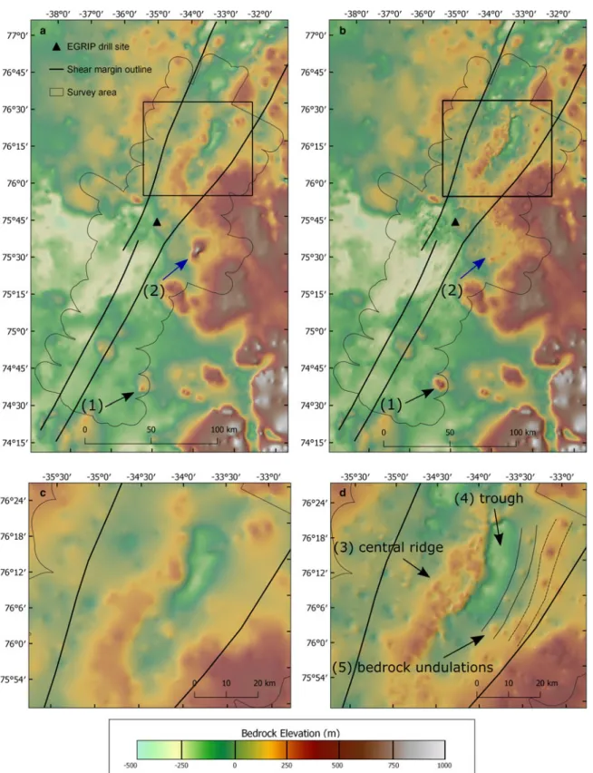
In comparison with the BMv3 bed the most prominent differences of our bed topography appear at different locations and show five main features:

(1) Figures 2band3aandbshow a location with elevation differences as large as 367 m. This isolated hill in the southeast of our survey area (indicated with a black arrow inFigs 3aand b) shows a higher basal elevation and larger surface area in the EGRIP-NOR-2018 topography in comparison with BMv3.

(2) A hill in the central southeast of our survey area, which is visible in the BMv3 bed topography (Fig. 2band marked with a blue arrow inFigs 3a andb) and roughly 20 km away from the eastern shear margin, is not present in our bed topography. At this position, we find no significant change in ice surface topography but a strong internal reflection above the bed (Fig. 4). The highest elevation of BMv3 at this point is 697 m higher than our bed elevation. Three survey lines cover this feature and reveal strongly folded isochrones in our echograms. An internal anticline extending up to 15 km along the track exhibits elevation differences of isochrones of more than 900 m (Fig. 4). Furthermore, this radargram shows a strong power return of a similar amplitude as the bottom reflector in the proximity of the anticline. This reflection is irregularly shaped with interruptions, steeply dip- ping flanks and shows multiple layering. Underneath this anticline, we observe a weaker reflection, which we interpret as the real bed echo.

(3) A longitudinal ridge in the center of the ice stream 35–90 km downstream of the EGRIP drill site is located 300–500 m higher than the surrounding bed. In contrast to BMv3, this topographic high is now represented as being more isolated from the high elevated area in the east, that coincides with the position of the eastern shear margin on its western edge. The ridge is oriented only a few degrees off from the direction of the surface ice flow of the NEGIS.

(4) Southeast of the ridge, we find a trough. The transition is marked by a high elevation gradient of up to 500 m over a distance of 2–5 km. The trough shows an increasing depth in the along-flow direction and ends abruptly with a 300 m elevation increase over a distance of 3 km.

(5) Further east of the trough our radar lines show isolated bed undulations, which are aligned in the ice flow direction and bend downstream toward the western shear margin. The shape of this alignment is similar to the eastern and western slope of the trough to the West.

Discussion

Large scale bed structures

The EGRIP-NOR-18 bed topography shows several structures which are not present in previous bed elevation models. This is mainly due to our increased density in line spacing than in former surveys. Previous radar survey lines by AWI and Operation IceBridge (OIB) only covered parts of our survey area. At feature (1) inFigures 3aandb, only the edge of the bed feature was covered by one former survey line. However, the profile lines of other surveys indicate that this structure does not extend further than 10 km to the East. Feature (2) inFigure 3ais an ice bottom track- ing error resulting from a strong reflection that does not represent the ice–bed interface (seeFig. 4).

Except for these larger scale differences between previously available datasets, the new nested bed elevation model mainly differs by more definition and steeper topographic gradients

(5)

afforded by the increased spatial resolution of our data. The steeper gradients stand out in the region downstream of the EGRIP drill site, where a ridge in the center of the ice stream and an adjacent trough toward the east are delineated by a 300 m drop in bed elevation over 2 km. These structures are oriented almost parallel to ice flow (labeled with 3 and 4 inFig. 3d). Further toward the east, the trough is bordered by a chain of bed undulations, which very likely form a connected ridge (Fig. 3d, features labeled 3, 4 and 5), also orientated roughly along ice flow. However, due to the lack of flow-parallel survey lines in this region this remains speculative. The trough shows the characteristics of an elongated, closed topographic depression: an overdeepening. These are common features in formally glaciated landscapes, and have been also documented underneath existing ice sheets and glaciers (e.g. Cook and Swift, 2012; Patton and others,2016). A section of the bed along a flow line shows the typical profile of an overdeepening over two terraces, with the deeper part shifted toward the head (upstream) and a gentler upward slope downstream in each part of the basin. This indicates ongoing erosion by quarrying on the upstream end, leading to further deepening (Cook and Swift, 2012). This geomorphology is usually more common toward the margins of the ice sheet, where large, fast-flowing outlet glaciers drain through confined valleys. Patton and others (2016) suggested that the overdeepening structures found in their analysis of the bed topography beneath the central part of the Antarctic and Greenlandic ice sheets might have been initiated in a period with a thinner ice layer, when the ice flow was more defined by the basal topography. The unusually high surface velocities of NEGIS, at least for the central region of the ice sheet, appear to facilitate ongoing erosion of the previously existing bed morphology. Patton and others (2016) also suggest that sedimentation of eroded material at the downstream end of the overdeepening would lead to a stabilization of the structure, preventing erosion downstream due to the softness of the sediment layer and thus, protecting the bed. This would then also

result in the flattening of the surface profile. In case of the NEGIS there is a distinct step in the surface elevation at the downstream boundary of the basin, which might be interpreted as the erosion material being effectively flushed away.

As noted before by Christianson and others (2014), the position and shape of the ice stream cannot be directly linked to the bed topography. The widening of the ice stream from a narrow channel with a width of 15 km upstream of the EGRIP Camp to a more than 50 km wide stream at the downstream end of our survey area is coincident with a 300 to 500 m step in the topography aligned perpendicular to the flow direction.

Interpretation of off-nadir reflections

For the major part of the survey area, the bed shows a clear reflection signature. Survey lines oriented transverse to ice flow show a variable bed topography with frequent elevation changes.

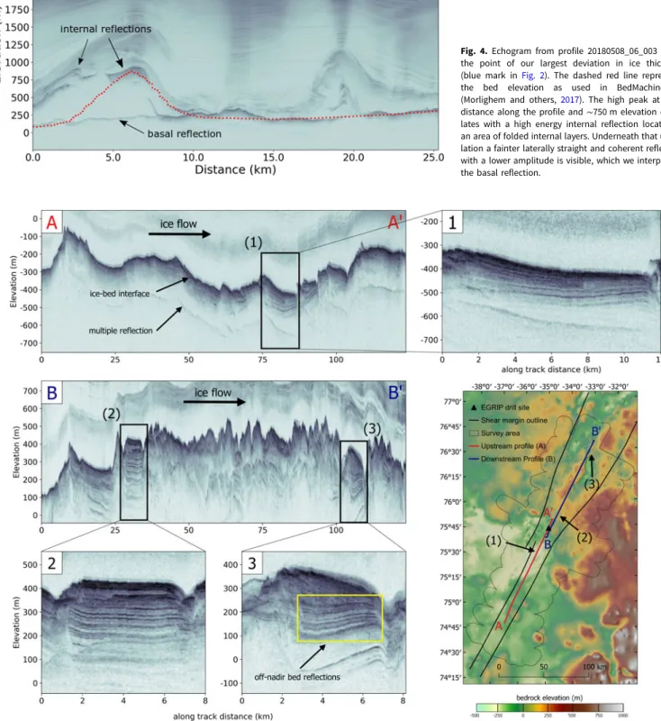
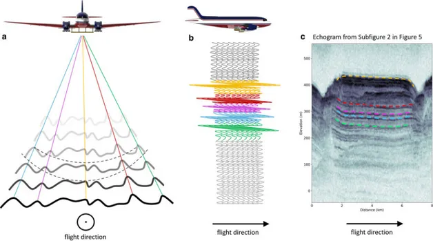
Radargrams parallel to ice flow show a smooth and straight basal reflection. Elevation changes appear as elongated steps rather than a pattern of ridges and troughs. Several of the along-flow radargrams show off-nadir events underneath the initial bed reflection (Fig. 5). These events are only found in survey lines from within the ice stream. We interpret them to likely be caused by side reflections off-nadir, that is by elevation changes in the across- track dimension.Figure 6shows a sketch of what kind of structures along the flight direction could generate these reflections in the radargrams. In some cases, we detect reflections in the form of straight lines, almost parallel and very similar to the shape of the primary bed reflection (subfigures 1, 2 and 3 inFig. 5). These features are too close to the primary bed event to represent multiple reflections. We argue that the topography in these areas shows elongated ridges oriented parallel to ice flow, which are not visible in the large-scale topography of Figure 3 because of a lack of adequate spatial coverage and data point density. Considering the geometry of the radar beam and the footprint at the base of

Fig. 2.(a) Map of ice thickness distribution based on the data of the AWI radar survey 2018, termed EGRIP-NOR-2018. EGRIP-NOR-2018 ice thickness minus BMv3 ice thickness is shown in the right image (b). Blue colors represent higher and red colors lower ice thickness in our dataset, respectively. The numbers 1–5 indicate the locations of the main features.

(6)

the ice sheet, the multiple reflectors could be generated by ridges with a height difference of tens of meters, and a ridge-to-ridge distance in the range of a hundred meters. However, on the basis of our data, this can only be evaluated qualitatively. These off-nadir reflection signatures are absent at the upstream end of our survey area, where ice-sheet velocity is below 30 m a⁻¹. They become more pronounced with increasing velocity in the downstream area, approximately around the EGRIP camp, where the ice stream begins to widen. They appear in the western trough as well as on

the central ridge. Unfortunately, there are no flow-parallel survey lines along the overdeepening in the east, so we cannot determine their presence. The structures have a length of up to 10 km (feature (1) inFig. 5A). It is possible that the ridges extend even further, as the flight trajectory might not be exactly parallel to the orientation of the structures, which would cause a fading of the reflections in the radar data and thus interruptions in their appearance. In most cases the main bed reflection along these features is very smooth, at constant depth or with a very gentle slope, while at the

Fig. 3.Bed topography of (a) BedMachine v3 (Morlighem and others,2017and (b) the EGRIP-NOR-2018 bed topography derived from our ice thickness data. A magnified view for the area upstream of the EGRIP drill site for both models (a and b) is shown on the two lower images (c and d, respectively). Two locations with strong elevation differences are marked with a black and blue arrow (feature 1 and 2). In the magnified sections, (c) and (d), we show the location of features 3–5. The black lines in feature 5 outline a possible connection of the single undulations.

(7)

downstream end of the multiple reflections a significant change in the bed slope can be detected (Figs 5AandB). This indicates that the flight line here is cutting the grooved bed at a small angle.

Thus, it is not possible to derive the exact along-flow extension of these features from the airborne data, but we can only provide a lower estimate.

The small-scale subglacial elongated landforms, which we deduce from the interpretation of side reflections, are probably a result of the flow activity of NEGIS in its current configuration, as they are parallel to the direction of observed surface ice flow.

Elongated ridges at the ice–bed interface of a similar scale have been mapped underneath active ice streams before. Holschuh and

Fig. 4.Echogram from profile 20180508_06_003 along the point of our largest deviation in ice thickness (blue mark inFig. 2). The dashed red line represents the bed elevation as used in BedMachine v3 (Morlighem and others,2017). The high peak at 6 km distance along the profile and∼750 m elevation corre- lates with a high energy internal reflection located in an area of folded internal layers. Underneath that undu- lation a fainter laterally straight and coherent reflection with a lower amplitude is visible, which we interpret as the basal reflection.

Fig. 5.A set of radargrams from the upstream (A) and downstream part (B) of the survey area oriented parallel to ice flow. The data were recorded with an increased radar cross-track beam angle. Subsections of the radargrams indicating the location of off-nadir reflections are shown in the radargrams 1, 2 and 3. An example of the off-nadir bed reflection pattern in the radargram is indicated in radargram 3 with the yellow outline. The position and the orientation of the radargrams (A to A^′in red and B to B^′in blue) as well as the location of the off-nadir reflection patterns 1, 2 and 3 are indicated in the map in the lower right corner.

(8)

others (2020) used swath radar data at Thwaites Glacier in Antarctica and mapped subglacial landforms which show a clear link between bedform orientation and ice flow. Jezek and others (2011) interpreted ridges underneath parts of the Jakobshavn Isbræ as linear erosion of a hard bed, a landform which is also known from previously glaciated areas (Bradwell and others, 2008). To create these structures high flow velocities and a significant sliding between ice and bed is required. However, data from a seismic survey close to the EGRIP Camp indicate a layer of soft, water saturated sediments beneath the main trunk of the ice stream.

Saturated deformable sediments are one facilitator of fast-flowing ice streams (Winsborrow and others,2010) which can produce elongated bedforms, such as MSGL (Stokes and Clark, 2002). Apart from areas with relict MSGLs, they have also been documented beneath active ice streams, for example in West Antarctica below the Rutford Ice Stream by King and others (2009), as well as below Pine Island Glacier (Bingham and others, 2017). MSGLs may be produced by either rapid ice flow over a short time, or slower ice flow over a longer duration (Stokes and Clark,2002).

We observe our features in areas of slow to moderate ice surface flow velocities of 30–80 m a⁻¹(based on surface velocities provided by Joughin and others,2018). This would indicate that these subglacial features can either form at lower flow velocities or that ice flow in this region has persisted for a long time or at higher velocities than at present, and that dilatant till is present over a wide area beneath the ice stream. It is also possible that there are transitions between hard-bedded eroded streamlined landforms to soft-bedded landforms caused by different basal lithologies or a changing dynamic activity over several glacial cycles. Without further evidence about the nature of the ice–bed interface this remains speculative.

Conclusion

A new high-resolution ice thickness dataset has been computed on the basis of airborne radar data. We derived a bed elevation model and analyzed topography related structures in the area of the NEGIS in the vicinity of the EGRIP drill site. Basal

topography is resolved in greater detail than in current bed elevation models of Greenland and covers a greater area than previous investigations and identified several misinterpretations of earlier ice thickness and thus bed elevation data. The enhanced resolution and more accurate geometry of the bed topography influences estimates of hydropotential and basal water routing. We observe an elongated topographic overdeepening, which indicates long-term erosion, potentially even over multiple glacial cycles.

Small-scale elongated subglacial landforms in the center of the ice stream oriented parallel ice flow probably cause off-nadir reflections in our radargrams. Due to the survey line spacing and without additional geophysical data, the nature and geomorphology of these structures cannot be determined further.

Either these landforms are formed by erosion in hard bed or by depositional processes, in which case they could represent MSGLs. The latter would also be consistent with the observations of Christianson and others (2014), who found a meter thick layer of sediment across the ice stream located in the vicinity to the locations where we identify these features. Another set of seismic profiles and a higher resolution of the bed topography in regions where we interpret our basal radar return as subglacial landforms would be helpful to evaluate our hypothesis in terms of the composition and structure of elongated bedforms and the existence of sediments. However, a full 3-D bed elevation model is basically a requirement to more comprehensively interpret areas where we find evidence for the types and formation subglacial landforms.

Nevertheless, our current analysis significantly improves previous bed elevation dataset in terms of coverage and accuracy, thus fos- tering more reliable ice flow model applications to investigate driving ice-dynamic process of NEGIS.

Data

The gridded ice thickness and bed topography data as well as the TWTs of the ice thickness along the radar profiles are available at the Data Publisher for Earth & Environmental Science (PANGAEA:https://doi.pangaea.de/10.1594/PANGAEA.907918).

Fig. 6.This sketch shows how the bed structures of our interpretation of basal off-nadir reflections can look like. (a) Side reflections are scattered toward the receiver from elongated landforms aligned parallel to the flight trajectory. The black lines represent the bed reflector at different positions along the flight path. The different off-nadir reflections, which are most likely caused by scattered reflections by the elongated structures, are shown here in five different colors.

(b) If the structure is parallel to the flight direction, a similar reflection pattern is recorded in the traces along the flight trajectory. (c) In the example of echogram section of the profile 20180515_01_007, the recorded signal could potentially look as indicated by the colored dashed layers. Plane model by courtesy of University of Kansas, Department of Engineering (2015).

(9)

and Marine Research), Japan (National Institute of Polar Research and Arctic Challenge for Sustainability), Norway (University of Bergen and Bergen Research Foundation), Switzerland (Swiss National Science Foundation), France (French Polar Institute Paul-Emile Victor, Institute for Geosciences and Environmental research) and China (Chinese Academy of Sciences and Beijing Normal University). We acknowledge the use of software from CReSIS generated with support from the State of Kansas, NASA Operation IceBridge grant NNX16AH54G, and NSF grant ACI-1443054.

The authors would like to thank Emerson E&P Software, Emerson Automation Solutions, for providing licenses in the scope of the Emerson Academic Program. We thank Martin Siegert and two anonymous reviewer for comments that improved the quality and readability of this manuscript.

Author contributions. Steven Franke wrote the manuscript and conducted the main part of the data processing and analysis. Olaf Eisen and Daniela Jansen were PI and Co-I of the campaign and designed the study. Daniela Jansen coordinated and conducted the field work together with Tobias Binder and John Paden. Veit Helm processed GPS data and assisted with further data processing together with Daniel Steinhage. John Paden and Nils Dörr contributed to the radar data processing with the CReSIS Toolbox and imple- mented the set-up for the nested bed elevation model. Daniela Jansen, Steven Franke and Olaf Eisen interpreted the radar and bed topography data. All co-authors discussed and commented on the manuscript.

References

Allen CT, Mozaffar SN and Akins TL(2005) Suppressing coherent noise in radar applications with long dwell times. IEEE Geoscience and Remote Sensing Letters2(3), 284–286. doi:10.1109/LGRS.2005.847931

Aschwanden A, Fahnestock MA and Truffer M(2016) Complex Greenland outlet glacier flow captured.Nature Communications7(May 2015), 1–8. doi:

10.1038/ncomms10524

Bamber JL and 10 others(2013) A new bed elevation dataset for Greenland.

Cryosphere7(2), 499–510. doi:10.5194/tc-7-499-2013

Bingham RG and 12 others(2017) Diverse landscapes beneath Pine Island Glacier influence ice flow. Nature Communications 8(1), 1618. doi: 10.

1038/s41467-017-01597-y

Bohleber P, Wagner N and Eisen O(2012) Permittivity of ice at radio fre- quencies: part II. Artificial and natural polycrystalline ice. Cold Regions Science and Technology 83–84, 13–19. doi: 10.1016/J.COLDREGIONS.

2012.05.010

Bradwell T, Stoker M and Krabbendam M(2008) Megagrooves and streamlined bedrock in NW Scotland: the role of ice streams in landscape evolu- tion.Geomorphology97(1–2), 135–156. doi:10.1016/j.geomorph.2007.02.

040

Christianson K and 7 others(2014) Dilatant till facilitates ice-stream flow in northeast Greenland.Earth and Planetary Science Letters401, 57–69. doi:

10.1016/j.epsl.2014.05.060

Church JA and 13 others(2013) 2013: Sea level change.Climate Change 2013:

The Physical Science Basis. Contribution of Working Group I to the Fifth Assessment Report of the Intergovernmental Panel on Climate Change, Cambridge, UK, pp. 1137–1216. doi:10.1017/CB09781107415315.026 Cook SJ and Swift DA(2012) Subglacial basins: their origin and importance

in glacial systems and landscapes.Earth-Science Reviews115(4), 332–372.

doi:10.1016/j.earscirev.2012.09.009

CReSIS-Toolbox(2019) J Paden. Available at https://ops.cresis.ku.edu/wiki/

index.php/Main{\_}Page, accessed: 2019-06-01.

Dowdeswell JA and 5 others (2014) Late Quaternary ice flow in a West Greenland fjord and cross-shelf trough system: submarine landforms from Rink Isbrae to Uummannaq shelf and slope. Quaternary Science Reviews92, 292–309. doi:10.1016/j.quascirev.2013.09.007.

Dutrieux P and 6 others(2013) Pine Island glacier ice shelf melt distributed at kilometre scales.Cryosphere7(5), 1543–1555. doi:10.5194/tc-7-1543-2013 Fahnestock M, Abdalati W, Joughin I, Brozena J and Gogineni P(2001) High geothermal heat flow, basal melt, and the origin of rapid ice flow in

thickness datasets for Antarctica.The Cryosphere7(1), 375–393. doi:10.

5194/tc-7-375-2013

Gardner AS and 14 others(2013) A reconciled estimate of glacier contributions to sea level rise: 2003 to 2009.Science340(May), 852–857.

Gazdag J (1978) Wave equation migration with the phase-shift method.

Geophysics43(7), 1342–1351. doi:10.1190/1.1440899

Gillet-Chaulet F and 7 others(2012) The Cryosphere Greenland Ice Sheet contribution to sea-level rise from a new-generation ice-sheet model.The Cryosphere6(6), 1561–1576. doi:10.5194/tc-6-1561-2012

Goelzer H and 41 others (2020) The future sea-level contribution of the Greenland ice sheet: a multi-model ensemble study of ismip6. The Cryosphere Discussions2020, 1–43. doi:10.5194/tc-2019-319

Gogineni S and 9 others(2001) Coherent radar ice thickness measurements over the Greenland Ice Sheet.Journal of Geophysical Research106(D24), 33761–33772. doi:10.1029/2001JD900183

Hale R and 6 others(2016) Multi-channel ultra-wideband radar sounder and imager center for remote sensing of ice sheets, University of Kansas Alfred Wegener Institute, Germany. 2016 IEEE International Geoscience and Remote Sensing Symposium (IGARSS), Beijing, China.

Hogan KA, Ó Cofaigh C, Jennings AE, Dowdeswell JA and Hiemstra JF (2016) Deglaciation of a major palaeo-ice stream in Disko Trough, West Greenland.Quaternary Science Reviews147, 5–26. doi:10.1016/j.quascirev.

2016.01.018.

Holschuh N, Christianson K, Paden J, Alley R and Anandakrishnan S(2020) Linking postglacial landscapes to glacier dynamics using swath radar at Thwaites Glacier, Antarctica.Geology48(3), 268–272. doi:10.1130/g46772.1.

Howat IM, Joughin I and Scambos TA(2007) Rapid changes in ice discharge from.Science315(5818), 1559–1561. doi:10.1126/science.1138478 Howat IM, Negrete A and Smith BE(2014) The Greenland ice mapping pro-

ject (GIMP) land classification and surface elevation data sets.Cryosphere8 (4), 1509–1518. doi:10.5194/tc-8-1509-2014

IPCC(2019)IPCC Special Report on the Ocean and Cryosphere in a Changing Climate[H.-O. Pörtner, Roberts, D. C., Masson-Delmotte, V., Zhai, P., Tignor, M., Poloczanska, E., Mintenbeck, K., Nicolai, M., Okem, A., Petzold, J. Rama, B. Weyer, N. (eds.)]. Technical report. doi:https://www.ipcc.ch/report/srocc/

Jezek K and 6 others(2011) Radar images of the bed of the Greenland Ice Sheet.Geophysical Research Letters38(1), 1–5. doi:10.1029/2010GL045519 Jezek K, Wu X, Paden J and Leuschen C(2013) Radar mapping of isunn- guata Sermia, Greenland.Journal of Glaciology59(218), 1135–1146. doi:

10.3189/2013JoG12J248

Joughin I, Smith BE and Howat IM(2018) A complete map of Greenland ice velocity derived from satellite data collected over 20 years. Journal of Glaciology64(243), 1–11. doi:10.1017/jog.2017.73

Joughin I, Smith BE, Howat IM, Scambos T and Moon T(2010) Greenland flow variability from ice-sheet-wide velocity mapping.Journal of Glaciology 56(197), 415–430. doi:10.3189/002214310792447734

Keisling BA and 8 others(2014) Basal conditions and ice dynamics inferred from radar-derived internal stratigraphy of the northeast Greenland ice stream.Annals of Glaciology55(67), 127–137. doi:10.3189/2014AoG67A090 Khan SA and 12 others (2014a) Sustained mass loss of the northeast Greenland ice sheet triggered by regional warming. Nature Climate Change4(4), 292–299. doi:10.1038/nclimate2161

Khan SA and 10 others (2014b) Glacier dynamics at Helheim and Kangerdlugssuaq glaciers, southeast Greenland, since the Little Ice Age.

Cryosphere8(4), 1497–1507. doi:10.5194/tc-8-1497-2014

King EC, Hindmarsh RCA and Stokes CR(2009) Formation of mega-scale glacial lineations observed beneath a West Antarctic ice stream. Nature Geoscience2(8), 585–588. doi:10.1038/ngeo581

Kjær KH and 21 others (2018) A large impact crater beneath Hiawatha Glacier in northwest Greenland. Science Advances 4(11), eaar8173. doi:

10.1126/sciadv.aar8173

Legarsky JJ, Gogineni SP and Akins TL(2001) of ice-sounder data collected over the Greenland Ice Sheet.October39(10), 2109–2117.

Leuschen C, Gogineni S and Tammana D(2000) SAR processing of radar echo sounder data.IGARSS 2000. IEEE 2000 International Geoscience and

(10)

Remote Sensing Symposium. Taking the Pulse of the Planet: The Role of Remote Sensing in Managing the Environment. Proceedings (Cat.

No.00CH37120), Honolulu, HI, USA, 2000, vol. 6, pp. 2570–2572. doi:

10.1109/igarss.2000.859643

Leysinger Vieli GM, Hindmarsh RCa and Siegert MJ (2007) Three-dimensional flow influences on radar layers stratigraphy.Annals of Glaciology46, 22–28.

Li J and 8 others(2013) High-altitude radar measurements of ice thickness over the Antarctic and Greenland ice sheets as a part of operation icebridge.

IEEE Transactions on Geoscience and Remote Sensing51(2), 742–754. doi:

10.1109/TGRS.2012.2203822

Martos YM and 5 others(2018) Geothermal heat flux reveals the Iceland hotspot track underneath Greenland. Geophysical Research Letters 45(16), 8214–8222. doi:10.1029/2018GL078289

Morlighem M and 31 others(2017) BedMachine v3: complete bed topography and ocean bathymetry mapping of Greenland from multibeam echo sounding combined with mass conservation. Geophysical Research Letters44(21), 11051–11061. doi:10.1002/2017GL074954

Mouginot J, Rignot E, Scheuchl B and Millan R (2017) Comprehensive annual ice sheet velocity mapping using Landsat-8, Sentinel-1, and RADARSAT-2 data.Remote Sensing9(4), 1–20. doi:10.3390/rs9040364.

Newton AMW and 6 others(2017) Ice stream reorganization and glacial retreat on the northwest Greenland shelf.Geophysical Research Letters44 (15), 7826–7835. doi:10.1002/2017GL073690

Patton H, Swift DA, Clark CD, Livingstone SJ and Cook SJ (2016) Distribution and characteristics of overdeepenings beneath the Greenland and Antarctic ice sheets: Implications for overdeepening origin and evolu- tion.Quaternary Science Reviews 148, 128–145. doi: 10.1016/j.quascirev.

2016.07.012.

Rignot E and Mouginot J(2012) Ice flow in Greenland for the international polar year 2008–2009.Geophysical Research Letters39(11), 1–7. doi:10.

1029/2012GL051634.

Rignot E, Velicogna I, Van Den Broeke MR, Monaghan A and Lenaerts J (2011) Acceleration of the contribution of the Greenland and Antarctic ice sheets to sea level rise. Geophysical Research Letters38(5), 1–5. doi:

10.1029/2011GL046583

Robel AA, Degiuli E, Schoof C and Tziperman E(2013) Dynamics of ice stream temporal variability: modes, scales, and hysteresis. Journal of Geophysical Research: Earth Surface118(2), 925–936. doi:10.1002/jgrf.20072 Roberts DH and Long AJ(2005) Streamlined bedrock terrain and fast ice flow, Jakobshavns Isbrae, West Greenland: implications for ice stream and ice sheet dynamics. Boreas 34(1), 25–42. doi: 10.1111/j.1502-3885.2005.

tb01002.x

Roberts DH, Long AJ, Davies BJ, Simpson MJR and Schnabel C(2010) Ice stream influence on West Greenland Ice Sheet dynamics during the Last Glacial Maximum.Journal of Quaternary Science25(6), 850–864. doi:10.

1002/jqs.1354

Robinson A, Calov R and Ganopolski A(2012) Multistability and critical thresholds of the Greenland ice sheet.Nature Climate Change2(6), 429– 432. doi:10.1038/nclimate1449

Rodriguez-Morales F and 17 others(2014) Advanced multifrequency radar instrumentation for polar Research.IEEE Transactions on Geoscience and Remote Sensing52(5), 2824–2842. doi:10.1109/TGRS.2013.2266415 Rogozhina I and 9 others(2016) Melting at the base of the Greenland ice

sheet explained by Iceland hotspot history.Nature Geoscience9(5), 366– 369. doi:10.1038/ngeo2689

Rückamp M, Goelzer H and Humbert A(2020) Sensitivity of Greenland ice sheet projections to spatial resolution in higher-order simulations: the AWI contribution to ISMIP6-Greenland using ISSM.The Cryosphere Discussions 2020, 1–26. doi:10.5194/tc-2019-329

Schlegel NJ, Larour E, Seroussi H, Morlighem M and Box JE (2015) Ice discharge uncertainties in Northeast Greenland from boundary conditions and climate forcing of an ice flow model. Journal of Geophysical Research: Earth Surface120(1), 29–54. doi:10.1002/2014JF003359 Shi L and 8 others(2010) Multichannel coherent radar depth sounder for

NASA operation ice bridge.International Geoscience and Remote Sensing Symposium (IGARSS), Honolulu, HI, USA, pp. 1729–1732. doi:10.1109/

IGARSS.2010.5649518

Stokes CR and Clark CD(2002) Are long subglacial bedforms indicative of fast ice flow?Boreas31(3), 239–249. doi:10.1111/j.1502-3885.2002.tb01070.x Truffer M and Echelmeyer KA(2003) Of Isbræ and ice streams.Annals of

Glaciology36, 66–72. doi:10.3189/172756403781816347

Vallelonga P and 22 others(2014) Initial results from geophysical surveys and shallow coring of the Northeast Greenland Ice Stream (NEGIS).Cryosphere 8(4), 1275–1287. doi:10.5194/tc-8-1275-2014

Wang Z and 13 others (2014) Wideband imaging radar for cryospheric remote sensing.International Geoscience and Remote Sensing Symposium (IGARSS), Quebec City, QC, Canada, pp. 4026–4029. doi: 10.1109/

IGARSS.2014.6947369)

Winsborrow MC, Clark CD and Stokes CR(2010) What controls the location of ice streams?Earth-Science Reviews103(1–2), 45–59. doi:10.1016/j.earscirev.2010.07.003

Wright AP, Siegert MJ, Le Brocq AM and Gore DB(2008) High sensitivity of subglacial hydrological pathways in Antarctica to small ice-sheet changes.

Geophysical Research Letters35(17), L17504. doi:10.1029/2008GL034937

Appendix A

Radar data processing

As a preliminary result, which is also generated in the field, we produce a quick look echogram with presumed unmigrated data. This output is used to automatically determine the ice surface location by using a maximum power layer tracker. CReSIS SAR processing algorithms use the surface location to model the ice as a layered media for fk migration (Leuschen and others,2000). A simple dielectric half-space is used for representing the layered media with a relative dielectric permittivity of ice of 3.15. Recorded radar signals of each channel are processed individually and stacked coherently, equivalent to beam- forming toward nadir. Depending on the number and pulse duration of the transmitted waveforms, different receiver gains are applied to increase the dynamic range. Radargrams with low and high gain are combined into a single image. The low gain echogram is used for the upper part of the image and the high gain echogram is used for the lower part of the image.

Pulse compression in the frequency domain is used to improve range resolution and SNR. As a result of this processing step, range sidelobes appear on both sides of the main return with a time window of twice the pulse duration (Li and others,2013). A Hanning window is applied in the frequency domain to suppress range sidelobes and both the transmit signal and the matched filter are tapered with a Tukey window in the time domain. Range resolution depends on the propagation speed of the radar wave, and thus on the real part of the relative permittivityεr, the bandwidth of the transmitted chirpB and a factor for window widening due to the frequency and time domain win- dows,ki, according to

d(r)= kic

2B√1r. (A1)

For the NB bandwidth of 30 MHz, the theoretical range resolution in ice withεr= 3.15 andki= 1.53 is 4.31 m.

Transmit equalization

Prior to the data acquisition, transmit equalization of the emitted radar signals was performed on open water on the transit to Greenland. Adjustment of coefficients for amplitude, phase and time delay for each transmitter and each receiver helps to compensate any mismatches caused by hardware. This adjustment is of particular importance for beam-focusing and array processing to increase SNR. The coefficients are determined during a test flight prior to the actual data acquisition.

Motion compensation

Fourier-based processing algorithms for SAR processing require a uniformly sampled linear trajectory of the receivers along the extent of the SAR aperture and high precision timing information. Any deviation from a straight line reduces the maximum possible SNR of the received signal and induces phase errors, which degrade the target focusing (Legarsky and others,2001).

Velocity variations, for instance, alter the along-track sampling and create an irregular sample spacing. High precision processed GPS and INS data from the aircraft are used to correct these effects. Before SAR processing, we (1) resampled the data in along-track using a windowed sinc interpolation ker- nel and (2) corrected any flight path deviations with a time delay.

(11)

2000). The processing uses signal information from adjacent traces and the result is based on the dielectric model of the subsurface to determine the radar wave propagation speed (Legarsky and others,2001). For the migration we use a layered velocity model with two constant permittivity values (ε= 1 for air andεr= 3.15 for ice). The air–ice interface is determined with an automatic surface tracker on unmigrated data. Time delays occurring due to changes of the aircraft trajectory and altitude are also corrected during this step (Rodriguez-Morales and others, 2014). The SAR aperture length at each pixel is chosen to create a fixed along-track resolution of 2.5 m.

Array processing

Coherent combination of return signals in the cross-track dimension is applied to increase SNR and to reduce surface clutter. For our processing, the antenna array beam is steered toward nadir. Since surface clutter due to crevasses is not prominent in our data, we applied the‘delay and sum’method for channel combination. This algorithm uses multi-looking of ambient pixels of the image pixel that is combined followed by along-track decimation (Jezek and others, 2013). To multilook, the array processed output is power detected and then averaged with neighboring pixels. In this case, the averaging window is 5 range lines before and 5 range lines after the current range line, resulting in reduced signal variance or fading and a coarser resolution of 2.5 m × 11 = 27.5 m along track. An output is generated every 6 range lines so that the sampling or posting in the final image is 2.5 m × 6 = 15 m.

whereHis the height of the aircraft over the ice surface andcthe speed of light. Our flights were all performed at an elevation of∼365 m above ground, which corresponds to a cross-track footprint of 300–350 m for an ice column of 2000–3000 m in our survey region. The bed return, however, is in some cases characterized by layover signals from off-nadir due to topography. In this case, cross-track resolution depends on the full beam width,βy, of the antenna array:

by=arcsinlc

Ndy

, (A3)

whereλcis the wavelength at the center frequency,Nis the number of array elements and dyis the element spacing of 46.8 cm. Cross-track resolution can now be calculated as

sy=2H+T 1

√ tanbykt

2 , (A4)

whereTis the ice thickness andktis the window widening factor which 1.53 for 20% Tukey time-domain window on transmit. Considering Eqn (A4) with a beam angle of∼21° corresponds to a cross-track resolution for the bed layer of 800 to 1100 m for an ice thickness range of 2000–3000 m.