Characterization of Reflection Seismic Systems in Glaciology by Data Analysis of the PALAOA-Observatory
Masterarbeit im Studiengang Geowissenschaften Fachbereich Geowissenschaften
Universität Bremen
angefertigt am
Alfred-Wegener-Institut für Polar- und Meeresforschung von
Maximillian Grahs Bremen, 2020
1. Gutachter
Prof. Dr. Olaf Eisen 2. Gutachter PD Dr. Karsten Gohl
Fachbetreuer:
Dr. Coen Hofstede
Abstract
With the critically intensifying global climate change the scientific interest in the Arctic and Antarctic increases continuously. Polar ice sheets are in a constant dynamic state and flow, depending on conditions of the subglacial bed. Information about the subglacial bed are important for estimating the ice sheet evolution and climate modelling.
Seismic observations are basic methods to estimate spatial and physical properties of the subglacial bed. Different parameters that depend on the material and system characteristics like the attenuation, reflection coefficient and source amplitude drive the behaviour of elastic waves and furthermore the assessment of the results in glaciology. This leads to large uncertainties in defining the subglacial material. The PALAOA observatory is a set of calibrated hydrophones placed within the water column beneath the Ekström Ice Shelf, Antarctica. Its main purpose is to identify the underwater sea life soundscape, but can also be used for recording seismic shots triggered at the ice surface. The unique location of the hydrophones provides new opportunities of observing seismic signals, due to different ray paths in comparison to conventional methods.
24 shots triggered by a Vibroseis truck at the ice surface at 6 different locations are analysed.
Ray paths and travel times of four signals of various reflections at each shot point are calculated and identified in the seismograms. The analysis of amplitudes of different signals in correlation with known properties of ice and water aims to provide estimations about attenuation of seismic waves depending on the shot point distance.
This thesis presents a new method for analysing seismic data. The results highlight, that the time delay between the first signal arrival and the highest amplitudes (main signal) of single shots increases with an increasing shot distance. This is caused by sp-converted waves at the ice – water interface. Amplitudes show a strong decrease with increasing offsets. Several uncertainties complicate the seismogram interpretation which are discussed. Finally this thesis depicts in a first approach, how the usage of hydrophones could complement methods in observations of seismic data in glaciology and further constitutes the basis of prospective future studies.
Kurzfassung
Der während der letzten Dekaden sich intensivierende Klimawandel verstärkt das wissen- schaftliche Interesse in das Verständnis polarer Regionen. Eisschilde in der Arktis und Antarktis fließen kontinuierlich in Abhängigkeit des sich darunter befindlichen Materials.
Genaue Kenntnisse über subglaziale Fazies sind eine wichtige Grundlage vergangener und zukünftiger Eisschild- und Klimamodellierung.
Seismische Untersuchungen dienen der Analyse räumlicher und physikalischer Eigenschaften des Untergrundes. Kenngrößen wie Dämpfung, Reflektionskoeffizient und Quellamplitude beeinflussen die elastischen Wellen und führen besonders in der Glaziologie zu Ungenauigkeiten, die eine Materialbestimmung des Untergrundes erschweren. Bei der PALAOA-Horchstation handelt es sich um Hydrophone, die unterhalb des schwimmenden Ekström-Eisschelfs in der Antarktis in der Wassersäule platziert sind. Sie können neben der Observation mariner Lebewesen auch der Aufzeichnung der mittels an der Eisoberfläche durch Vibrationen ausgelösten seismischen Signale genutzt werden. Die besondere Lokation der Hydrophone ermöglicht eine neue Strategie zur Untersuchung seismischer Signale durch andere Laufwege im Vergleich zu herkömmlichen Methoden. Mittels Laufzeitberechnungen können einzelne Signale in den Seismogrammen zugeordnet werden. Die Messung der Amplituden verschiedener Signale liefert im Einklang mit bekannten physikalischen Eigenschaften von Eis und Wasser Informationen über die Dämpfung in Abhängigkeit des Laufweges.
Die Arbeit präsentiert eine neuartige Messmethode zur Analyse seismischer Studien. Die Untersuchung der Seismogramme weist einen zunehmenden Versatz zwischen Ersteinsatz und Hauptsignal mit starken Amplituden mit zunehmender Entfernung der Schusspunkte auf. Dies lässt sich mit der Ankunft von an der Eisunterkante sp-konvertierten Wellen erklären. Die Amplituden verschiedener Signale zeigen deutliche Abnahmen mit zunehmenden Laufwegen.
Die durch die neuartigen Grundlagen entstehenden Komplexitäten werden mit der Arbeit aufgezeigt. Abschließend veranschaulicht die Arbeit den möglichen Nutzen der Hydrophone als vielversprechendes Messelement und bildet die Grundlage neuer Studien.
Danksagung
An dieser Stelle möchte ich mich bei all denjenigen bedanken, die mich während der Masterarbeit unterstützt und mir diese ermöglicht haben.
Zunächst gilt mein Dank Herrn Prof. Dr. Olaf Eisen für die Bereitstellung des äußerst interessanten Themas, für die Begutachtung der Arbeit sowie die schnelle Beantwortung meiner Fragen.
Ebenso möchte ich mich bei Herrn PD Dr. Karsten Gohl bedanken, der die Zweitprüfung übernommen hat.
Ganz besonderer Dank gilt meinem Betreuer Herrn Dr. Coen Hofstede, der mich während des gesamten Bearbeitungszeitraums unterstützt hat und stets für Fragen bereit stand. Ebenso stand er in häufigem Kontakt mit weiteren Mitarbeitern, um beispielsweise das Prozessingproblem mit Paradigm zu beheben, oder offene Fragestellungen zu beantworten.
Weiterhin möchte ich mich ganz herzlich bei meiner Familie bedanken, sowie bei meinen Freunden: Jerry, Yannis, Cedric, Kai und Andi, die nicht nur ein offenes Ohr für Fragen bezüglich der Arbeit hatten, sondern auch stets für die notwendige Ablenkung sorgten. Danke euch!
Außerdem gilt ganz besonderer Dank an Judith, die mich während der gesamten Masterarbeit unterstützt und ermutigt hat.
Ich danke euch allen ganz herzlich.
Acknowledgement
The author would like to thank Emerson E&P Software, Emerson Automation Solutions, for providing licenses for the seismic software Paradigm in the scope of the Emerson
Academic Program
Erklärung gem. § 10 Abs. 11 Allg. Teil d. Master-PO vom 27.10.2010
Ich versichere hiermit, dass ich meine Masterarbeit selbständig verfasst und keine anderen als die angegebenen Quellen und Hilfsmittel benutzt habe. Wörtliche oder dem Sinn nach aus anderen Werken entnommene Stellen sind unter Angabe der Quellen kenntlich gemacht.
Die Arbeit wurde nicht in einem anderen Prüfungsverfahren eingereicht.
Weiterhin erkläre ich, dass die Masterarbeit in unveränderter Fassung der Öffentlichkeit zur Verfügung / nicht zur Verfügung* gestellt werden kann. *Zutreffendes bitte markieren
Bremen, 13.05.2020__________ __________________________
Ort, Datum Unterschrift
Table of Contents
1. Introduction ... 1
1.1. Structure of ice sheets and ice shelves ... 3
1.2. Densification from firn to ice ... 6
1.3. Seismics in glaciology – state of the art ... 7
1.4. Motivation and structure of the thesis ... 9
2. Theoretical background ... 11
2.1. Seismic waves ... 12
2.1.1. Body waves ... 12
2.1.2. Surface waves ... 13
2.2. Wave propagation characteristics ... 14
2.3. Seismic source ... 18
2.3.1. Vibroseis signal ... 18
2.3.2 Cross-correlation ... 20
2.4 Receivers ... 21
2.4.1 Surface geophones ... 21
2.4.2 PALAOA hydrophone ... 22
3. Database and Methodology ... 23
3.1 Field site ... 23
3.2 Data acquisition and measurement setup ... 24
3.3 Travel time and ray path calculations ... 27
3.4 First arrival analysis ... 32
3.5 Amplitude calculation ... 33
4. Results ... 34
4.1 Timing correction and geometry ... 35
4.2 Ray paths and travel times ... 36
4.3 Event detection ... 40
4.4 Event Amplitudes ... 43
5. Discussion and Interpretation ... 50
5.1. Geometry and velocities ... 50
5.2. Seismogram interpretation ... 52
5.3. Error analysis of event arrival times ... 54
5.4. Amplitude interpretation ... 58
5.5. Critical discussion ... 61
6. Conclusion ... 63
7. Outlook ... 64
8. Bibliography ... 65
9. Appendix A ... 70
1. Introduction
With the critically intensifying global warming since the beginning of the pre-industrial era at the middle of the 19th century, the interest in scientific questions and observations of the polar regions increases constantly. Over this timespan, the average worldwide temperature rose by about 1.0 °C and it accelerates with an increasing rate especially during the last 30 years (IPCC Special Report on Global Warming; Masson-Delmotte et al., 2019). The evolution of the temperature differs depending on the location. It increased more than twice as much at the poles than on the global average within the last two decades (IPCC SROCC; Pörtner et al., 2019, in press). The polar ice sheets in the Arctic and Antarctic would not only cause a global sea level rise of about 65 m due to their immense size if they would melt (Cuffey and Paterson, 2010), but they would also indirectly impact the whole worldwide ecosystem. Because ice acts as a kind of mirror that reflects solar radiation back into the space, the energy and heat will not be absorbed in the atmosphere and the environment. If ice is melting, the mass changes its state of aggregation from brighter ice or snow to darker water. Whereas ice or snow-covered surfaces have a high albedo (a parameter that characterizes the strength of backscattering solar radiation) of 68-90%, water has an albedo of less 30-35 % so the ocean absorbs the radiation of the sun instead of reflecting it like ice or snow (Kishtawal, 2013). Less ice causes less backscattering and thus more heat is absorbed in the atmosphere, cryosphere and hydrosphere and that increases the temperature that furthermore decreases the ice covered areas so the processes amplify themselves.
Because polar regions are very important for the worldwide ecosystems, scientists of different specialisations like geophysicists, meteorologists, chemists etc. around the world perform local scientific campaigns for in situ (in direct, natural state) observations for a better understanding of the processes that drive the behaviour of ice sheets. All different aspects of the cryosphere have to be taken into account to connect the information and finally make assumptions of future ice sheet development and sea level rise. There are three kinds of the ice masses like inner ice sheets, ice shelves (floating part of the ice) or continental glaciers. Different properties affect the dynamic state of ice sheets like spatial distribution, mass balance, internal structures and the subglacial bed. Several methods are used to examine the most important physical parameters like snow accumulation rate, surface and basal melting, temperature and density profiles and further flow velocity and strain rates. Furthermore, in addition to the analysis of ice, the physical properties of the subglacial bed like basically spatial distribution, density, porosity, roughness and water content are exceedingly important, because the dynamic features of ice sheets are facilitated by sliding or motion at their beds or deformation of the ice above the subglacial bed (Smith and Murray, 2009). Because of the spatial extent of the East Antarctic ice sheets of more than 1000 kilometres in length and width and a thickness up to 4500 m
maximum (Lüthi et al., 2017), only point measurements by drilling are possible to reach direct contact to the subglacial bed. Boreholes are cost-intensive, time consuming and just give a local point information. However, they can provide a lot of detailed information that can be combined with geophysical methods.
Seismic is a geophysical method commonly used and base on the propagation of elastic waves.
It is used to display and analyse the internal spatial structures and layering of englacial and subglacial material (Booth et al., 2013). A seismic source transmits elastic waves triggered by an Air-Gun offshore, in polar cases with an impulse source like explosives charges or with vibroseismic trucks (Vibroseis). The waves penetrate into the ground and be reflected at an interface of two different media. Geophones placed at the surface record the incoming seismic signals and provide information about the ground like its thickness or velocity. Due to a lack of specific quantitative knowledge about the effective source amplitude, attenuation and reflection coefficient of seismic campaigns on ice, scientists often make several assumptions that cause large uncertainties that prevent an accurate identification of the subglacial material (Holland and Anandakrishnan, 2009). Especially the attenuation of the waves within the ice is an important factor based on its sensitivity to lithology, anisotropy, fluid content, porosity and temperature (Peters et al., 2012).
The Perennial Acoustic Observatory in the Antarctic Ocean (PALAOA) Observatory now consists of two calibrated hydrophones that are arranged in the ocean cavity below the Ekström Ice Shelf in East Antarctica. After Kindermann et al., (2008) PALAOA contained originally four hydrophones but two of them are now defect. Since 2005 the hydrophones observe the underwater soundscape of marine sea life below the ice shelf (Kindermann et al., 2008). In 2010 seismic shots and Vibroseis sweeps were triggered on the ice surface that were recorded by the PALAOA hydrophone. By analysing the records of vibroseismic shots, only one way travel time downwards the hydrophone has to be examined. The aim of the thesis is to characterize the acoustic records of PALAOA by observing the amplitudes of different seismic events and further to quantify the source amplitude and the amount of the attenuation by traveling of the waves through the ice shelf. The amplitudes of several reflections will be compared with the results of the surface geophones, in dependence of an increasing offset. Finally the work aims to decrease the general uncertainties in seismic surveys in glaciology like the source amplitude and the attenuation of the seismic waves through the ice.
1.1. Structure of ice sheets and ice shelves
Fundamentals of glaciers
In the following discussion ice sheets and glaciers are described after Benn and Evans (2010).
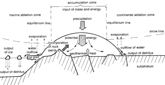
Glaciers can be divided into three main types: ice sheets and ice caps (unconstrained by topography), glaciers constrained by topography and ice shelves. Furthermore several subclasses like outlet glaciers, ice domes, valley glaciers etc. exist. Glaciers basically contain a mass gaining (accumulation zone) and a mass dispensing (ablation zone) area. They are divided by the equilibrium line of altitude (ELA) which position depend on the location and height of the glacier as well as climate and geographical factors. The accumulation zone has an annual average positive mass balance, so the snowfall or windblown snow as a form of precipitation adds more mass to the region as it is losing by surface and basal melting. The ELA marks the line where the annual accumulation is in equilibrium with the annual ablation. The accumulation zone is accordingly located at the inner and / or higher elevation part of the glacier or ice sheet (Figure 1) with extents for hundreds of kilometres in length and width and some kilometres in height (Kuhn, 1995). The ablation zone contains in the most cases the lower (and older) part of the glacier as well as the floating ice shelves. In the ablation zone the glacier loses mass. The distribution of the accumulation and ablation zone and finally its flow behaviour describe the dynamic state of the glacier (Cuffey and Paterson, 2010; Benn and Evans, 2010). The ice divides (ID) are boundaries with an opposing ice flow direction. Whereas the flow along the ice divide is zero, it is on either sides orientated in the opposite direction (Benn and Evans, 2010). The flow direction depends on the surface slope orientation and the
Figure 1: Sketch of different domains in an ice sheet (Brodzikowski and van Loon, 1990).
gravitational force. The ice flows from the ID towards the coast where the ice starts sliding in form of ice streams. When the ice streams pass the grounding line (the area that marks the boundary between grounded and floating ice) they become floating ice shelf. Ice shelves will be explained in detail in the following.
Ice Shelves
Ice shelves are floating ice masses and fringe about 74% of the Antarctic’s coastline (Hogg and Gudmundsson, 2017). They are the interacting part between the land ice and the ocean. As the ice is already floating and displacing water, it is calving or “break off”, so the loss of larger ice bergs or melting, does not directly affect the global sea level. Ice shelves act as a barrier that buttress the grounded ice masses located upstream (Hogg and Gudmundsson, 2017). Calving
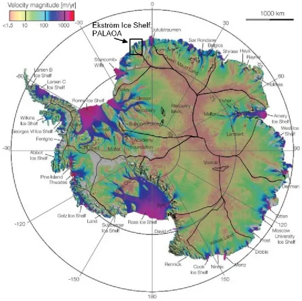
Figure 2: Map with flow velocities of the Antarctic ice sheets modified after by Rignot et al., (2011). Ice shelves at the surrounding edge of the continent show higher velocities than the inland ice sheets. Black lines mark ice divides. Ekström ice shelf and the location of PALAOA is mentioned in the black rectangle.
of ice shelves causes an acceleration of grounded ice (Rignot et al., 2004) and thus increases the masses adding to the ocean that once again affect the global sea level. One example is the giant break off in 2017 of the new ice berg A18 at the Larsen C ice shelf on the Antarctic Peninsula (Hogg and Gudmundsson, 2017).
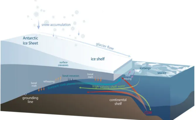
Different processes at the surface and the base impact the state of ice shelves. Ice has fluid and elastic properties. The flow of ice can be described by internal deformation, basal sliding and soft bed deformation caused by dipping angles of the subglacial bed, basal melt and the gravitational force (Jiskoot, 2011). Several processes drive the effective anisotropy of the ice in ice shelves. The top layer consist of snow or ice crystals including a high amount of air particles in the pores. Furthermore fabric anisotropy is caused by the stress regime with higher depths (Diez et al., 2014). Melting and refreezing in the upper firn constitute different layers with changing sizes and formations of crystals up to the surface. Finally a consequent densification with depth builds a single layer with different densities and velocities that consequences will be explained later.
Percolating warmer ocean currents may melt ice at the base of the shelf. On the other hand the ice can refreeze water once again. Freezing and melting changes the volume of the ice shelf and furthermore the fresh water content and thus the ocean water conditions (Marshall and Speer,
Figure 3: Sketch of an ice shelf with its state driving processes (modified after Padman et al., 2018).
2012). Surface rifts can be reinforced by basal and surface melting that are possibly followed by ice berg calving (Figure 3).
1.2. Densification from firn to ice
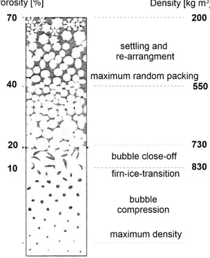
The surface of glaciers commonly consists of freshly fallen or wind transported snow. With adding mass and force by settled snow the densification and transformation process to ice begins. The porosity and content of air bubbles decreases with depth while the grain size increases (Cuffey and Paterson, 2010). Freshly fallen snow under calm conditions accumulates with a density of 50-200 kg/m³ due to its high porosity (Figure 4). Settled snow that survived one melt season without being transformed into ice is called firn (Cuffey and Paterson, 2010;
Benn and Evans, 2010). Firn has a density of 430 – 800 kg/m³ (Cuffey and Paterson, 2010).
With increasing depth a gradual increase in density occurs up to the maximum density of pure ice that is about 917 kg/m³ (Benn and Evans, 2010) and thus lower than the density of water. After Herron and Langway (1980) and Arnaud et al. (2000) three main stages of densification exist during the transformation from firn to ice. The first and main stage occurs up to a “first critical density” of ρ = 550 kg/m³ (Figure 4). Getting to this density, the shape of the snow crystals changes from dendritic, hexagonal flakes to spheres by adhesion because of the principle of the state of smallest free energy (Arnaud et al., 2000;
Benn and Evans, 2010). Further the almost perfect spheres slide at each other and decrease the porosity to 40% to a maximum random packing. At the second stage, the
interconnected air bubbles get separated to single bubbles because of the continuative densification (Herron and Langway, 1980). The third stage, below the pore close-off zone, describes the mechanical compression of the separated and conserved air bubbles. At this stage the firn has a density of >830 kg/m³ and is called ice (Herron and Langway, 1980).
Finally the maximum density of pure ice at a temperature of 0° C and low pressures is ρ = 917 kg/m³. For massive polar ice sheets with lower temperatures and higher pressures because of
Figure 4: Different densification stages from firn to ice (modified after Blunier and Schwander, 2000)
their immense size, the maximum density can vary up to 922 kg/m³ (Cuffey and Paterson, 2010).
1.3. Seismics in glaciology – state of the art
Several studies with seismic campaigns were carried out in different regions and glaciers during the last decades. Explosive shots within a borehole were always common. In addition a vibration system (Vibroseis) was used for the first time by the Alfred-Wegener-Institut für Polar- und Meeresforschung (AWI) in 2010, also a detonation cord became more feasible later (Hofstede et al., 2013). The first applications at the beginning of the 21th century prove that a vibrator as a seismic sources works on ice in the Antarctic (e.g. Eisen et al., 2010a (unpublished report);
Kristoffersen et al., 2010; Hofstede et al., 2013; Eisen et al., 2015). In comparison to explosive shots, a vibration system has some benefits. While for detonation charges holes with a depth of 2-5m have to be drilled (Hofstede et al., 2013), that is time consuming, a vibration system is a fast repeatable method for seismic profiling. It is also non-pollutive and decreases risks and transport effort (Hofstede et al., 2013). Furthermore explosive shots create a noisy signal called
“ghost” that describes a wave moving up to the ice surface and then downwards creating holes in the frequency spectrum (Eisen et al., 2010a) that does not occur with sources triggering shots at the surface like Vibroseis. On the other hand in comparison to explosive shots, the frequency bandwidth of a vibrator is limited for higher frequencies so the resolution of explosives is superior that makes englacial reflections more clearly visible (Hofstede et al., 2013). Over a long time period of studying the technique of seismic campaigns is being proved for its meaningful and accurate predictions about spatial conditions in glaciology. Several studies during the last decades depict the importance about uncertainties regarding to different physical parameters that will be explicated below.
Subglacial reflection coefficient
Seismic waves triggered at the surface propagate through the ice column and reflect or refract at an interface. The reflection coefficient gives the relative amplitudes (so the ratio) of the incident and reflected waves (Dobrin and Savit, 1988). A lack of knowledge of the absolute source amplitude and the attenuation of the waves causes uncertainties in calculating the reflection coefficient that further makes it impossible to absolutely identify a subglacial material (Holland and Anandakrishnan, 2009).
The angle dependent reflection coefficient can be calculated with the receiver amplitude, the source amplitude, the ray path and the attenuation. Holland and Anandakrishnan (2009)
described new methods to calculate englacial reflection coefficients without a prior knowledge of the source amplitude or the englacial attenuation. A number of previous studies like Smith (1997; 2007) and others used calculations based on dependences between attenuation and energy. One method is to quantify the changes in energies between multiple bed reflections based on the assumption that the attenuation does not change within normal incident angles (Smith, 1997). Holland and Anandakrishnan (2009) illustrated the important difference between linking the attenuation to the amplitude instead of the energy. The attenuation is defined relative to the amplitude (Sheriff and Geldart, 1995). Because the amplitude ratio is the square root of the energy ratio (Dobrin and Savit, 1988), this causes wrong estimations about the reflection coefficient at the interface of ice the subglacial material. The second approach is the direct path method where the offset-dependent decrease of the amplitude of the arriving direct wave along the surface is observed. With respect to the spherical divergence the ratio of the amplitudes of different distant receivers can be extrapolated and give information about the source amplitude.
Temperature dependence of attenuation
Holland and Anandakrishnan (2009) mentioned the need to know the seismic attenuation α of seismic waves. Without a prior knowledge about the attenuation it is not possible to distinguish between a crystalline rock and unconsolidated sediments as a subglacial material (Holland and Anandakrishnan, 2009). Peters et al. (2012) further showed the sensitivity of the attenuation or internal friction to the temperature regime within the ice column and the ice crystal orientation.
Using a spectral ratio method they calculated the seismic quality factor Q and generated a temperature profile with depth. They show results with a good agreement between their calculated temperature profiles dependent on the quality factor and given temperature profiles of boreholes. Peters et al. (2012) showed that their method can be used to determine the thermal regime within an ice sheet that further enables the evaluation of the attenuation. Because they link their results to existing borehole data, it is difficult to make general estimations as boreholes are cost intensive and only give point measurements. Furthermore Peters et al. (2012) disregarded uncertainties by the undefined absolute coupling to the ground as described by Holland and Anandakrishnan (2009). The unique location of the PALAOA Observatory gives the motivation of the thesis.
PALAOA Observatory
The Ekström Ice shelf (EIS) is well studied because of the German scientific station Neumayer III and the previous Neumayer II station. Several seismic surveys on the EIS were executed (e.g.
Eisen et al., 2010a; Hofstede et al., 2013; Kristoffersen et al., 2014). In 2005 four hydrophones were set up beneath the ice shelf to study the underwater soundscape (Kindermann et al., 2008).
First impressions show that the hydrophone is able to record seismic shots and finally becomes the fundamental idea of this thesis. As it is different to other seismic campaigns, the coupling of the hydrophone to the surrounding water is very good. The reflection coefficient that is exceedingly important for seismic analysis in this study is well known.
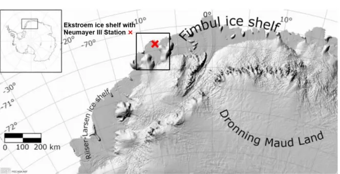
Figure 5 (upper): The map shows the survey area located on the Ekström Ice Shelf in Dronning Maud Land in the Antarctic. The red cross marks the location of the Neumayer III Station (modified after Jacobs et al., 2019). Lower, left: Configuration of PALAOA (Kindermann et al., 2008). Lower, right: Vibroseis sweep recorded with the PALAOA hydrophone on 4th February 2010 (Eisen et al., 2010a).
1.4. Motivation and structure of the thesis
Because of the location and configuration of the PALAOA hydrophone this thesis presents a new way of analysing glaciological seismic data on ice. Several uncertainties are common in glaciological seismic surveys on ice like the source energy that penetrates into the ice and the amount of seismic attenuation.
The primary aim of the thesis is to interpret the seismograms recorded by one PALAOA hydrophone (Figure 5) and calculate amplitudes of different event arrivals, e.g. the direct wave or seafloor reflection. For this, the ray paths and travel times of different events will be calculated before. During the survey in 2009/10 also a surface geophone streamer was used. The approach of the streamer data is to get an overview about the ice thickness along the shot points and ice shelf and further the seismic velocity in the ice shelf. Details about the source, geophone streamer and hydrophone configuration are mentioned in chapter 3. This is important to get the basics of the geometry of the ray paths and the velocity of the seismic waves. Before calculating travel times, the spatial conditions have to be reviewed.
Given that the hydrophone is placed in the water column, the seismic waves follow a ray path that enables a new way of observing and analysing their physical properties. With well-known values of ice and water density and velocity and Snell’s Law (1621), the travel times of different events can be calculated. Three different amplitudes will be calculated: (1) Maximum Amplitude (Max), (2) Root-Mean-Square Amplitude (RMS) and (3) Average Amplitude (Avg.) within different time gates at the time of arrival of the different events. In combination with the shot geometry with increasing offsets (= distance between source and receiver / hydrophone) to the fixed PALAOA hydrophone the changes of amplitudes are analysed to give an outlook about the impact of the attenuation of the seismic waves through the ice column and the representation of the results as an alternative way to advance seismic on ice shelves.
2. Theoretical background
Figure 6: General remarks of seismic campaigns on ice shelves (white) floating on sea water (blue) with thicknesses matching the spatial conditions on Ekström Ice Shelf. The source P(t) transmits seismic waves with a wavefront (red lines) and the travel path L (red dashed lines) that propagate through the media in the ground where they reflect based on the reflection coefficient (R(p) at the ice-water interface) and move back towards the receivers P(r) (modified after Eisen et al., 2010a). The incident angle i depends on the position of the source and the particular receiver.
The main purpose of seismic observations is the determination of different lithology’s and their thicknesses and physical properties. The setup of the surveys consists of a source and receivers.
Sources can vary in type of signal triggering but all function aiming an identical purpose.
Receivers are generally geophones or hydrophones (in marine seismics) placed as a group within a streamer so a single shot is measured by a plurality of receivers. With an assumed velocity and the downward – upward travel time, the two-way traveltime (TWT), of the reflected waves the proper subsurface structure can be constructed.
The seismic wave field consists of two different types of waves (body waves and surfaces waves), each separated into two subclasses (body waves = compressional and shear waves; surface waves
= Rayleigh- and Love-waves). Body waves propagate through a medium away from the surface and surface waves arise at an interface of two media like the earth’s surface and move along them. In all cases the propagation takes place by an elastic displacement of particles but in a different direction of motion of the particles with respect to the direction of wave propagation.
Each of the four types of seismic waves follows Huygen’s Principle (1678) of wave propagation.
The principle indicates that in a single medium every point of a wavefront can be regarded as a new spherically spreading wave front (Dobrin and Savit, 1988; Lowrie, 2007). In a homogenous, isotropic medium, the wavefront spreads spherically with a constant curvature at the same time and distance to the source where all particles vibrate in the same phase. As the energy from a point source spreads spherically with increasing distance r, the energy decays with a factor 1/r² and the amplitude, being proportional to the root of the energy, decays with a factor 1/r.The
loss in energy and amplitude caused by the spreading of the wavefront is called spherical divergence and its correction is a basic part in seismic data processing (Yilmaz, 1987) (in Figure 6 is r = L). The direction perpendicular to the wavefront is the raypath and a central part of observation and analysis in this work. The physical properties of the different waves will be explained in the following.
2.1. Seismic waves 2.1.1. Body waves
Body waves can be classified into compressional and shear waves.
Compressional or longitudinal waves have the highest velocity of all wave types within the same medium and are the first or primary (P-waves) waves arriving in seismometers or geophones (Haldar, 2013). The direction of the particle motion is the same as the direction of propagation of the wavefront (longitudinal) so they are one-dimensional waves (Figure 7). Let the moving direction 𝐹 of the wavefront 𝐴 be the x-axis (Figure 7), the medium experiences a stretching and compressing parallel to the x-axis. The distance between the particles in x-direction changes. P-waves appear in all three phase states of a medium (solid, fluid, gas). The
velocity of compressional waves depends on the elastic moduli and can be expressed after Lowrie (2007) as:
𝑣 =
µ
,
(2.1.1)with the bulk modulus k, the shear modulus μ and the density ρ.
Figure 7: The propagation of compressional (P-waves) occurs in a strechting and compressing of the medium (upper part) parallel to the moving wavefront direction (x- axis in the lower part) (Lowrie, 2007).
Shear or transversal (S-waves) waves are the second type of body waves but differ in their properties to compressional waves.
The particle motion does not occur in a stretching and compressing parallel to the direction of propagation but perpendicular to it in y- or z-direction (Lowrie, 2007).
There are two types of shear waves. 𝑆 waves describe shear waves with particles moving in a vertical direction, whereas 𝑆 waves indicate a horizontal particle motion (Figure 8). The velocity of shear waves can be expressed as:
𝑣 = µ
.
(2.2.2)The parameters are explained in equation 2.2.1 above. Because the shear modulus becomes zero in liquids and gases, S-waves only occur in rigid bodies (Lowrie, 2007). The bulk modulus stays always positive so the velocity of shear waves is lower than for P-waves (𝑣 𝑣 ) so they occur later in seismograms or at geophones but with higher energies.
2.1.2. Surface waves
There are two types of surface waves named Rayleigh- and Love waves that differ in their particle motion (Figure 9). Whereas P-waves swing one-dimensionally in propagation direction and S- waves two-dimensionally in the propagation direction and vertically (𝑆 ) or horizontally (𝑆 ) perpendicular to it, the surface
waves can be regarded as a combination of both (Lowrie, 2007). The particles within a Rayleigh-wave experience a combination of a P-wave and a 𝑆 -wave and move in a retrograde ellipse perpen- dicular to the surface. Love- waves propagate parallel to the free surface and perpendicular
Figure 8: Shear or transversal waves (S-waves) occur with a horizontal or vertical movement of the particles perpendicular to the propagation direction through a solid medium (modified after Steeples, 2005)
Figure 9: Particle motion of Love- and Rayleigh waves (surface waves) in dependence of the propagation direction (modified after Steeples, 2005).
to the propagation direction as a combination of a P-wave and 𝑆 -wave. Surface waves occur at surfaces and interfaces and move with lower velocities along it. They are frequency dependent and have the highest amplitudes and energies and are visible in seismograms showing up as large and responsible for damages.
2.2. Wave propagation characteristics Acoustic Impedance
As mentioned before propagating seismic waves follow Huygen’s Principle (1678). This implies that each ray has a unique travel path and is calculated by the medium velocity and the time after the shot was fired. Figure 10 shows a spherically spreading wavefront propagating in a medium. A basic assumption for simplified ray paths is that the medium is homogeneous and isotropic so its density and the acoustic velocity or the orientation of the particles does not change within the medium. As the wavefront propagates spherically the rays move in every direction of all three dimensions with the travel path r (Telford et al., 1991; Lowrie, 2007). The energy and amplitude of the waves depends on the travel path r. When a seismic shot was fired at the surface of a solid medium (e.g. on an ice shelf) the P- and S-waves propagate into the ground through different media with changing physical properties. The acoustic impedance Z of a medium is given by its density ρ and velocity v and defined as:
Z = ρ*v. (2.2.3)
At an interface of two media with an abrupt change in their acoustic impedance reflection and transmission takes place (Figure 11).
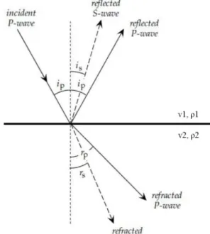
Snell’s Law
An incident P- or S-wave reflects at a media interface and travels back to the upper surface. The angle of incidence 𝜃 (in Figure 11 it is 𝑖 ) is equal to the angle of reflection. The amplitude decreases depending on the acoustic attenuation and travel path and furthermore the reflection coefficient that is also depending on the angle of incidence. A refracted wave propagates into the lower medium at a media interface and changes its angle of travel path according on Snell’s law:
=
.
(2.2.4)Snell’s Law depends on the sine of the incident angle 𝜃 and the velocity 𝑣 of the upper medium and the refracted angle 𝜃 and velocity 𝑣 in the lower medium (Dobrin and Savit, 1988; Lowrie,
2007). The angles 𝜃 and 𝜃 are directed to the lot perpendicular to the layer boundary (in Figure 11 it is 𝑖 , and 𝑟, ). An incident P-wave can also be converted into a refracted S-wave at the layer interface (P-S-Conversion) and inverse (S-P-Conversion).
Diving waves
Diving waves occur in regions where the density is constantly increasing within a single medium like firn. A diving wave is a constantly refracted wave, as Snell’s law predicts. This makes the waves propagate in a different ray (Figure 12). Diving waves occur in seismic data in the upper part so they can overlay and disturb important signals like direct waves or reflections. For sweeping signals of a Vibroseis this can be decreased as the energy is propagated
directional downwards. Figure 12: Travel path of diving waves within a single medium caused by constant changing density and / or velocity (e.g. on an ice shelf) (Diez, 2013).
Figure 11: An incident P-wave creates different kinds of refracted and reflected waves at a layer interface where physical properties (density and / or velocity) change (modified after Lowrie, 2007).
Figure 10: When a seismic shot is triggered with a source at the point P the waves propagate on a sphere in every dimension with the distance r to the source. The spherical wavefront is built by body and surface waves (Lowrie, 2007).
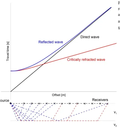
Travel time curves
Different types of waves have different characteristics. The direct wave propagates directly from the source to receiver. Direct waves are the first signals in receivers and useful for calculating seismic velocities of the medium. With lower offset and thus shorter travel paths of the seismic waves the first arriving signal at the receiver is the direct wave. With increasing offsets at a critical point the critically refracted wave overtakes the direct one because of its higher velocity in the lower medium (in two layered media conditions with 𝑣 < 𝑣 (also Figure 13)). The reflected waves are the last signals and not arriving in a linear delay with respect to the offset but as a hyperbole caused by the normal move out (NMO) that will be explained later (Figure 13).
Reflection (RC) and transmission (TC) coefficient at normal incidence
As similar to reflected waves, the amplitude of refracted waves changes depending on the physical properties. Because in this study the hydrophone stays in the lower medium, the transmission coefficient is important. The reflection and transmission coefficients depend on the acoustic impedance Z. Near normal incidence angles up to about 15 ° do not make significant changes in the amplitude (Lowrie, 2007), but with increasing angles (larger offsets, so larger distances between the source and receiver), the reflection coefficient changes. Then,
Figure 13: Travel time curves of direct, reflected and refracted P-waves (upper part) and their travel paths within a homogenous and isotropic medium (2 layers) and 𝑣 <
𝑣 (lower part).
the partitioning of energies at a media interface follows the Zoeppritz-Equations, a set of complex equations (Aki and Richards, 2002; Dobrin and Savit, 1988). The reflection angle is always equal to the incident angle because the medium velocity is the same (Dobrin and Savit, 1988). In case of normal incidence the ratio of reflected energy 𝐸 and incident energy 𝐸 of two media is given by the impedances (equation 2.2.3) according to:
²
². (2.2.5)
The square root of equation 2.2.5 depicts the amplitude ratio of the incident and reflected waves and thus the reflection coefficient R of incident waves at an interface of two media. The reflection coefficient can be positive or negative due to the velocity or density of the lower medium. If the velocity is lower than in the upper medium the reflection coefficient contains a 180° shift phase and becomes negative (Dobrin and Savit, 1988). It can be recognized by the following equation:
𝑅 = . (2.2.6)
The reflection coefficient is given by the impedance 𝑍 , velocity 𝑣 and density 𝜌 of the upper medium and the impedance 𝑍 , velocity 𝑣 and density 𝜌 of the lower medium.
After Holland and Anandakrishnan (2009) the reflection coefficient especially for seismics in glaciology should be calculated in an alternative way with the following equation:
𝑅 𝜙 r 𝜙 𝑒 . (2.2.7)
Here the angle dependent reflection coefficient 𝑅 𝜙 depends on the source amplitude 𝐴 , the receiver amplitude 𝐴 , the ray path r and the temperature dependent wave attenuation α. The equation is more specific as the very dominant and important attenuation α is taken into account.
The transmission coefficient T gives the amplitude change of traveling waves caused by different velocities of two media. The transmission coefficient stays always positive and can be calculated with equation 2.2.8. The sum of R and T at an interface is always 1. Variables match that ones in equation 2.2.6.
TC = = (2.2.8)
2.3. Seismic source
2.3.1. Vibroseis signal
Vibrator seismic (Vibroseis) is commonly used on land, as it is non-destructive, non-pollutive and a fast reducible method. The AWI in Bremerhaven was the first and the only institute using vibration systems in glaciology (Kristoffersen et al., 2014; Polom et al., 2014). There are some difference between other conventional methods. First is the duration of a Vibroseis signal known as a sweep with a time duration T of several seconds. Thus the analysis and interpretation of the data is different to other methods as the generated sweep has to be cross-correlated with the source sweep to make amplitude peaks in time or frequency domain visible (chapter 2.3.2).
There is a better source control using a baseplate in comparison to explosive charges. Further the motion of the plate is purely vertical so the signal penetrates efficiently downwards. Because the source is at the surface, there is no ghost as mentioned before that disturbs the signal. In most cases a Vibroseis truck on ice by the AWI is used with a geophone streamer behind it.
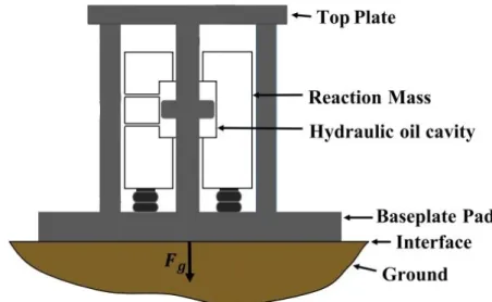
Preparation and signal triggering just takes several minutes as soon as the shot point (SP) is reached (Eisen et al., 2010a). The driving force is generated by an electrodynamic, hydraulic or magnetic system applied to the baseplate that is connected with a top plate and a reaction mass (Figure 14) (Baeten, 1989). The connection of the baseplate to the ground depends on the ground conditions like roughness and porosity.
Figure 14: Sketch of the operating method of a seismic vibrator system (Modified after Huang et al., 2018).
A sweep consists of a sine wave with a linearly increasing frequency (Figure 15). An increasing frequency leads to a decrease in the wavelength, the mathematical form of a sweep can be expressed [After Baeten (1989)] as:
s(t) = a(t) sin [2πθ(t)] , (2.3.1) with the sweep signal s(t), a taper function a(t) and the time dependent frequency function θ(t).
The amplitude stays at the same value during the sweep generation. The taper function reduces mathematical errors at the edge of filtering known as the Gibbs’ phenomenon that describes a ringing caused by the Fourier transformation.
Figure 15: Example of a sweep triggered by a Vibroseis with a linearly increasing frequency range from 1 to 5 Hz over a time gate of 8 seconds (modified after Braile, 2016).
Figure 16: Synthetic linear sweeps with a taper function of 0.5 seconds (upper) and 5 seconds (lower) (Brittle et al., 2001).
2.3.2 Cross-correlation
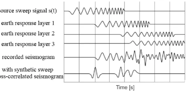
To make the source signal of Vibroseis shots visible, a cross-correlation has to be applied. It is a standard method to filter the original signal out of the seismogram. The source sweep signal s(t) with the time duration T penetrates with a linearly increasing frequency into the ground.
Different layers with abrupt changing impedances reflect the source signal to the receiver that sums all incoming reflected signals at different interfaces within a timespan (Figure 17
“recorded seismogram”). A cross-correlation of two identical sweeps is an auto-correlation.
Using the cross-correlation, a synthetic signal with the same fundamentals of the source sweep (T = 10 s, frequency range: 10 – 100 Hz were used during the data acquisition this thesis deals with) superimposes the recorded seismogram over time. If the synthetic sweep completely matches the recorded signal, the cross-correlation sums the multiplication of both signals. This creates a time dependent signal with peaks that represent the summed amplitude of different reflection events. A large positive peak represents a nearly complete match of the earth responded source sweep and the synthetic one. Because the whole sweeps are multiplied and summed, the resulting amplitudes become very large on the orders of 10 and higher (e.g.
amplitudes of explosive charges are in orders of 1-10).
Figure 17: Sketch of the principle of a cross-correlation. A source sweep (pilot sweep) with a linearly increasing frequency reflects at exemplary different layers as earth response. The lowest graph shows the seismogram of the input trace cross-correlated with a synthetic sweep (modified after Lindseth, 1968).
2.4 Receivers
2.4.1 Surface geophones
In general seismic waves are recorded by geophones on land and by hydrophones in marine observations. Geophones detect arriving energy in form of ground motion transformed into an electrical impulse (Onajite, 2013). The geophone contains a magnet within a coil creating a permanent magnet field. Arriving seismic waves accelerate the magnet relatively to the coil caused by ground motion. This induces a voltage proportional to the particle motion in the ground (Onajite, 2013). Because the measured energy of a single geophone is very small, several geophones are grouped together in a channel. Furthermore ground roll of surface waves that disturb the results can be decreased. Thus, the sum of amplitudes within one phase that matches the length of the geophone chain becomes zero (Figure 18). On the other hand this configuration has a disadvantage: With large offsets the wavefronts arrive in low angles at the geophones that induces spatial aliasing. To avoid this, the streamer configuration was changed (explained in chapter 3). A number of channels with a given distance to each other are grouped together in a streamer. This allows the record of a single shot with several geophones along a distance at the
Figure 18: Ground roll suppression by eight geophones grouped in a channel (Hofstede et al., 2013).
surface. The electric signals are transferred to the data acquisition, including analogue to digital conversion.
2.4.2 PALAOA hydrophone
In contrast to the grouped channels of geophones in a streamer the PALAOA station has a different setup. PALAOA contains actually two active hydrophones of which one is used for this work. The exact location is shown in chapter 3 (Figure 20, 21, 24). The hydrophone is a Teledyne Reson TC4033 Spherical Reference Hydrophone (Eisen et al., 2010b, unpublished report). It measures the acoustic waves triggered by the seismic source using a piezoelectric sensor element. The piezo effect describes an electric signal generated by the movement of electric charges. Basically there are two regions in the element: one partially positive loaded and one partially negative loaded. Without any impacts the loads are balanced so there is no electricity. If a seismic or acoustic wave arrives at the enclosing membrane the piezo element gets compressed and the two partially loaded regions are moved with respect to each other.
Thus, on both sides an excess of electrical load arises and triggers an electrical signal. The acquired signal is calibrated and thus directly proportional to the sound pressure level in the water. The hydrophone has a frequency range from 1 Hz – 140 kHz with a sensitivity of -203 dB re 1μPa/V.
Figure 19: Schematics of Teledyne Reson TC4033 Spherical Reference Hydrophone. It consists of a piezoelectric sensor element that builds the acoustic centre. It is coupled to a cable that is connected with digital systems at the ice surface (modified; from: http://www.teledynemarine.com/reson-tc-4033; last call: 21.04.2020)
3. Database and Methodology 3.1 Field site
Figure 20: The map shows the survey area located on the Ekström Ice Shelf in Dronning Maud Land in Antarctica.
The red cross marks the location of the Neumayer III Station (modified after Jacobs et al., 2019).
The data was acquired during the LIMPICS (Linking micro-physical Properties to macro features in ice sheets with geophysical Techniques) ANT 2009/10 campaign that was focussed on a Vibroseis survey on the Ekström Ice Shelf (EIS) and a seismic survey with explosive charges in combination with low-frequency radar Halfvarryggen ice dome (HID) (LIMPICS). The Ekström Ice Shelf is located in the East Antarctic at the north-western Dronning Maud Land (DML) (Figure 20) and thus part of the Antarctic coastal zone. With a size of about 6800 km² the Ekström Ice Shelf measures about 60 km in east-west direction and 120 km from north to the south so it is a comparatively small ice shelf (Neckel et al., 2012). The shelf reaches into the Atlantic Section of the southern ocean. Several studies estimates an average ice thickness of about 100 m at the edge of the shelf increasing to almost 1000 m towards the inland ice sheet. The underlying water column exhibits thicknesses of about 160 m at the area of interest
Figure 21: Location of seismic shots during LIMPICS ANT 2009/10 campaign between the PALAOA hydrophone and Neumayer III Station. Red circles mark explosive shots, black dots show Vibroseis shots (Eisen et al., 2010a).
(Sandhager and Blindow, 2000; Kindermann et al., 2008; Eisen et al., 2010a; Smith et al., 2020).
On the EIS different surveys were operated. At PALAOA two surveys from the 4th to the 6th of February 2010 with different streamer configurations were operated. One of them was operated in the south of Neumayer III Station (STR) between the 29th of January and the 2nd of Feburary but not recorded with PALAOA The data used for this work was acquired between the PALAOA hydrophone at the northern edge of the shelf and the Neumayer III Station that is positioned 15 km to the south (Figure 21) named as the PALAOA Traverse (PTR). The exact locations of the shots are shown in Table 2.
3.2 Data acquisition and measurement setup
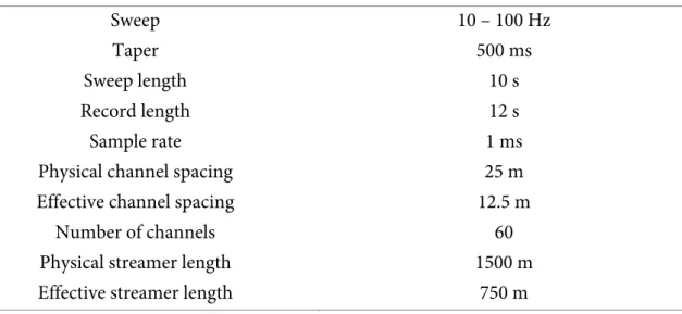
The seismic shots were acquired with the Failing 1100 Vibrator Vibroseis truck of the University of Bergen with a full weight of 16 tons (Eisen et al., 2010a). The data were recoded with a 60 channel streamer. Eight 14 Hz geophones (gimballed SM4 geophones) build one channel. The use of a streamer is very important for amplitude studies and the information about the ice and water velocity and thickness. The shot information is listed in Table 1.
The streamer was placed behind the truck with a distance (=offset) of 44 m between the first geophone and the source. The streamer has had a full length of 1500 m including 60 channels with a spacing of 25 m. Because the upper 500 m was the zone of interest, the streamer was towed in a loop so reflections in deeper regions will not arrive the geophones. It was also applied to minimize the channel spacing and thus spatial aliasing. This creates an effective streamer length of 750 m with a channel spacing of 12.5 m. Therefore, channel 30 has had the largest offset to the source while channel 60 was the closest one (see Figure 23). Two sweeps were triggered at every shot point (SP). After two shots the truck moved by 6.25 m (as half the distance of two channels) while the streamer stayed at the same position and another two shots were triggered. This simulated a 120 channel streamer with a spacing of 6.25 m and 4 shots per SP. The distance between groups of four shots was 375 m.
Altogether 98 shot points with each two sweeps were triggered in this streamer configuration.
The source generated a sweep with a 10 second duration and a frequency range of 10 to 100 Hz and a sample rate of 1 ms. Data were recorded with the surface geophones with a length of 12 seconds.
The first shot was located 130 m in the North of PALAOA and the survey direction was to the southern in direction of the Neumayer III station (see Figure 24). The PALAOA data on the other side was not coupled to the source so the data for the work are audio files converted into segy-data by Dr. Veit Helm (AWI) with a record length of 20 seconds and a different sample rate of 0.5 ms that include the shot signal (Figure 22).
Table 1: Source and receiver setup information during PTR in February 2010.
Sweep 10 – 100 Hz
Taper 500 ms
Sweep length 10 s
Record length 12 s
Sample rate 1 ms
Physical channel spacing 25 m
Effective channel spacing 12.5 m
Number of channels 60
Physical streamer length 1500 m
Effective streamer length 750 m
Figure 22: One explosive shot (left) and Vibroseis sweep (right) recorded with PALAOA at the 4th February 2010 (Eisen et al., 2010a)
The streamer configuration is illustrated in the following.
Figure 23: Streamer configuration during the PALAOA Traverse data acquisition (modified after Hofstede et al., 2013
Figure 24: The Figure shows the first 5 shot points with each 4 shots (each 2 points with a distance of 6.25 m).
Between every signed shot point is a distance of 375 m. The red star beneath PALAOA shows the locations where the hydrophone is placed in the water column (modified after Eisen et al., 2010a).
Several processing steps from the streamer data were applied by Dr. Emma Smith and Dr. Coen Hofstede at AWI to create a seismic profile. This was used to get a visual overview of the research area and to compare the thickness of the ice shelf and the water column with the calculated values of the single shots (chapter 4.1). The processing steps will not be explained here because it was not part of the thesis. We used the first six sweep locations of the PTR profile recorded by PALAOA hydrophone. Every sweep locations contains four sweeps. Detailed information about the different shots are shown in Table 2 below.
Table 2: Detailed information of several shots including their coordinates, time of triggering [UTC] and horizontal distance to PALAOA hydrophone [m]. Date of data acquisition was the 4th of February 2010.
Shot Point Shot name Time [hh:mm] PALAOA Offset [m]
1 PTR001a 20.41 130
1 PTR001b 20.45 123.75
2 PTR002a 21.50 247
2 PTR002b 21.53 253.25
3 PTR003a 22.24 615
3 PTR003b 22.27 621.25
4 PTR004a 22.52 991
4 PTR004b 22.54 997.25
5 PTR005a 23.19 1369
5 PTR005b 23.21 1374.25
6 PTR006a 23.53 1774
6 PTR006b 23.56 1780.25
3.3 Travel time and ray path calculations
Several studies roughly indicate values but especially the mean P- and S-wave velocities within the ice body need to be accurately known. To calculate the correct ray paths and travel times, detailed information about the thickness and velocity of the ice and water body are necessary.
To accomplish this, we use the streamer data. With familiar source and streamer geometry, the P- and S-wave velocities can be calculated in a first step. The velocities are necessary for calculating further the ice shelf thickness and the depth of the seafloor. All four shots of each of the first six shot points are spectated. Figure 25 below shows the first two shots of the survey (PTR001b) acquired with the 60 channel snow streamer, processed by Dr. Emma Smith and Dr.
Coen Hofstede.
To calculate the compressional and shear wave velocity within a medium, the direct P-wave and direct S-wave can be examined. Both are identifiable by a linear trend in time and distance.
Other reflections are visible as hyperbola (see Figure 25 and also Figure 13 in chapter 2.2). As the Vibroseis truck is located at the surface, the direct waves travel along a ray path at the snow surface to the geophones. Its velocity v can be calculated by the equation:
𝑣 , = = = (3.3.1)
The variable x indicates the distance s [m] and y gives the travel time t [s]. Note, that Figure 25 shows the two-way travel time but for calculating the velocity, one-way travel time has to be used. To get values for 𝑥 , and 𝑦 , a horizon can be picked (Figure 25) along the identified P- and S-wave. Every shot point contains 2 locations with a distance of 6.25 m (Table 2). Because this displacement has no significant impact on the whole travel path of the seismic rays, both locations (e.g. PTR001a and PTR001b) build one shot point and its offset to PALAOA is assumed to be 130 m. Each shot contains 2 vibration shots, so every shot point contains 4 shots (e.g. shot point one contains 2 shots at PTR001a and PTR001b). The shot with the best visible data at every shot point was used to calculate the velocities. This gives six values for the P- and S-wave velocity in ice and the ice thickness along the survey direction.
The ice base marks the interface between the ice shelf layer and the water column. To get information about the ice thickness, two different signals can be used: the difference of the multiple P-wave reflection of the ice base and the seafloor reflection and further the S-wave reflection of the ice base. The reflection from the ice base of the P-wave can’t be used because its arrival superimposes with several surface waves so it is quite difficult to distinguish between the signals. Both signals are visible as hyperbolic reflections in the data. The reflection from the ice base of the S-wave occurs later because of its lower velocity. The ice base reflection of the S- wave is very distinctive because of the high amplitudes of the S-waves. By converting the equation 3.3.1 the ice shelf thickness can be calculated with now familiar information about the velocity and the two travel time through the ice shelf.
Figure 25: Shot gather of Vibroseis shots 3, 4 (PTR001b) measured by the surface streamer containing 60 channels.
Dashed red lines mark direct waves and reflections caused by P- and S-waves. X-axis shows resorted streamer channel numbers 1-60, y-axis shows two-way travel time in seconds.
In the streamer data, the direct P-wave is characterized as the first arriving signal and constitutes a linear signal in the shot gather, followed by later arriving and bended diving waves (Figure 12). The direct S-wave and surface waves are also characterized by a linear shape but with a larger time delay and higher amplitudes. The direct S-wave is faster than the surface waves.
Reflections occur in a hyperbolic shape caused by the Normal Move Out (NMO). This is clarified by an increasing time delay of a horizon (e.g. the ice base reflection) because of the increasing travel path caused by an increasing distance of the channels to the source.
Because the PALAOA hydrophone stays within the water column, the rays follow a different travel path as if they are recorded with surface geophones. The rays propagate through the ice shelf layer into the water column refracted based on Snell’s Law (chapter 2.2). The theoretical ray paths are derived below. The simplest path is the direct one, which is just refracted at the ice – water interface and thus different to the direct wave recorded by surface geophones. Other ray paths, (=“events”) which include multiple reflections, and their travel times can be theoretically calculated, according to the actual geometry (Figure 26-28).
Figure 26: Rays of P-waves which propagate from the shot point at the ice surface to the PALAOA hydrophone through the ice shelf and are refracted at the ice base. Based on their different travel path, the traveltime of different events can be calculated. The reflection and refraction angles do not match the real values because the sketch just illustrates the theoretical shape of the ray paths. Colours indicate different paths with the names indicated as used in the text.
The geometry of the PALAOA experiment is well constrained, because the lateral and vertical position of the hydrophone is known as well as the ice shelf thickness and water depth, so the theoretical ray paths and travel times of different events can be calculated. The ray paths can be calculated theoretically by dividing them into two areas given by the ice shelf and water column medium. As shown in Figure 27, the ray path can be expressed as the hypotenuse of two rectangular triangles whose shapes are based on the incident and refracted angle at the ice – water interface, which again depends on the medium velocities and Snell’s Law.
Figure 27: Mathematical principle for the P-wave ray path and travel time calculation. The ray path corresponds the hypotenuse of two rectangular triangles in the ice and water column and thus became the sum of c1 and c2.
The angles within the triangles base on θ1 and θ2 that once again base on the seismic velocities.
Because the interfaces at the ice – air, ice – water and water – seafloor are assumed to be perfectly horizontal, the triangles comply the principle of Pythagoras so the hypotenuses of the triangle in the ice becomes (Figure 27):
𝑐 = 𝑎 ² 𝑏 ². 3.3.2
With the distances a, b and c, and for the triangle in the water:
𝑐 = 𝑎 ² 𝑏 ². 3.3.3
Because of geometrical conditions, the incident angle 𝜃 matches α in triangle 1 (in the ice).
The angle 𝛽 is given with respect to the knowledge of 𝛼 and 𝛾 . Because the distance 𝑏 matches the available ice thickness, the distance 𝑎 (further “Offset ice”) can be calculated with:
𝑎 = ∗ . 3.3.4
Therefore the hypotenuse 𝑐 becomes the combination of equations 3.3.2 and 3.3.4 as:
𝑐 = 𝑏1sin β ∗sin α1
1 𝑏 ². 3.3.5
Comparable conditions are valid in triangle 2 in the water. The angle of refraction 𝜃 is known to depend on Snell’s Law. With respect to rectangle conditions, 𝛽 becomes
𝛽 = 180° - 𝜃 𝛾 , with 𝜃 𝛼 . 3.3.6
The distance 𝑏 matches the depth of the PALAOA hydrophone. The information is given by Kindermann et al. (2008) and Eisen et al. (2010a). Therefore, the distance 𝑎 forms the “Offset water” and can be calculated with:
𝑎 = ∗ . 3.3.7
As in equation 3.3.5, the hypotenuse 𝑐 becomes the summary of equation 3.3.3 and 3.3.7 as:
𝑐 = 𝑏2sin β ∗sin α2
2 𝑏 ². 3.3.8
Finally the ray path x becomes the sum of both hypotenuses (equation 3.3.5, 3.3.8) as:
x = 𝑏1sin β ∗sin α1
1 𝑏 ² + 𝑏2sin β ∗sin α2
2 𝑏 ². 3.3.9
With given parameters for ice shelf 𝑏 and water column 𝑏 thickness, velocities for each medium and the offset (horizontal distance between the shot points and PALAOA location, the sum of 𝑎 and 𝑎 ), there is just one possible ray path that exactly reaches the hydrophone. Its ray path can be calculated with respect to Snell’s Law. All calculations can be found in the appendix. Three more events are characterized: (1) The ray path “Multiple” that travels from the source to the ice base, reflecting back to the surface, reflecting again at the ice – air interface
and then propagates to the PALAOA hydrophone with a refraction at the ice – water boundary.
(2) The event “Seafloor” that describes a ray refracting at the ice – water interface and then reflecting at the seafloor. (3) The finally event is the “Ice Base” that follows the “Seafloor” event and afterwards reflecting back at the water – ice interface down to the PALAOA hydrophone (Figure 26).
As the sweeps generated both P- and S-waves, we also derived the ray paths for generated S- waves which were converted into P-waves at the ice - water interface. The experiment has the same geometry (source, hydrophone location etc.) but the shear waves have a lower velocity in ice than compressional waves in water. This leads to different incident and refracted angles at the ice – water interface and so the ray paths theoretically follow a geometry as schematically shown in Figure 28 below.
Figure 28: S-waves propagate from the shot point at the ice surface to the ice base and cause a SP-conversion. In the water column they continue as P-waves to the PALAOA hydrophone. Basing on their different travel path, the travel time of different events can be calculated. The relations, reflection and refraction angles do not match the real values because the sketch just illustrates the theoretical shape of the ray paths.
3.4 First arrival analysis
The PALAOA hydrophone records continuously. The data provided for the study are converted segy-files of the audio data of PALAOA that contain a time window of 20 seconds that include the Vibroseis sweep. There is no synchronisation between the hydrophone and the source