Controlled-source electromagnetic and seismic delineation of subseafloor fluid flow structures in a gas hydrate province, offshore Norway

(1)

Geophysical Journal International

Geophys. J. Int.(2016)206,1093–1110 doi: 10.1093/gji/ggw188

Advance Access publication 2016 May 20 GJI Marine geosciences and applied geophysics

Controlled-source electromagnetic and seismic delineation of subseafloor fluid flow structures in a gas hydrate province, offshore Norway

Eric Attias,

¹

Karen Weitemeyer,

¹

Tim A. Minshull,

¹

Angus I. Best,

²

Martin Sinha,

¹

Marion Jegen-Kulcsar,

³

Sebastian H¨olz

³

and Christian Berndt

³

1Ocean and Earth Science, National Oceanography Centre Southampton, University of Southampton, European Way, Southampton,SO14 3ZH, UK. E-mail:eric.attias@noc.soton.ac.uk

2National Oceanography Centre, University of Southampton Waterfront Campus, European Way, Southampton,SO14 3ZH, UK

3GEOMAR Helmholtz Centre for Ocean Research Kiel, Marine Geodynamics, Wischhofstr.1-3, 24148Kiel, Germany

Accepted 2016 May 16. Received 2016 April 16; in original form 2015 November 17

S U M M A R Y

Deep sea pockmarks underlain by chimney-like or pipe structures that contain methane hydrate are abundant along the Norwegian continental margin. In such hydrate provinces the interaction between hydrate formation and fluid flow has significance for benthic ecosystems and possibly climate change. The Nyegga region, situated on the western Norwegian continental slope, is characterized by an extensive pockmark field known to accommodate substantial methane gas hydrate deposits. The aim of this study is to detect and delineate both the gas hydrate and free gas reservoirs at one of Nyegga’s pockmarks. In 2012, a marine controlled-source electromagnetic (CSEM) survey was performed at a pockmark in this region, where high- resolution 3-D seismic data were previously collected in 2006. 2-D CSEM inversions were computed using the data acquired by ocean bottom electrical field receivers. Our results, derived from unconstrained and seismically constrained CSEM inversions, suggest the presence of two distinctive resistivity anomalies beneath the pockmark: a shallow vertical anomaly at the underlying pipe structure, likely due to gas hydrate accumulation, and a laterally extensive anomaly attributed to a free gas zone below the base of the gas hydrate stability zone. This work contributes to a robust characterization of gas hydrate deposits within subseafloor fluid flow pipe structures.

Key words: Marine electromagnetics; Seismic tomography; Electrical anisotropy; Gas and hydrate systems.

1 I N T R O D U C T I O N

Methane hydrates are ice-like crystalline solids composed of water and gas that may form in marine sediments where a biogenic or thermogenic methane source is available, and remain thermo- dynamically stable under high-pressure and low-temperature con- ditions (Kvenvoldenet al.1993; Kvenvolden1998; Sloan & Koh 2007). Hydrate deposits are typically located between the seafloor and maximum depth extent of 135–1000 meters below seafloor (mbsf), within water depths that range from 400 to 4500 m (Kven- volden1988,1993). Estimates for the global inventory of submarine gas hydrate fall in the range∼500–3000 GtC (Buffett & Archer 2004; Milkov2004; Archer2007), later updated to about 1000 GtC (Archeret al.2009). More recent estimates based on transfer function models suggest a worldwide inventory of biogenic hydrate in marine sediments that ranges between∼455 and 550 GtC (Wall- mannet al.2012; Pineroet al.2013). Regarding the global recover-

able quantity of marine hydrates, Boswell & Collett (2011) propose gas-hydrate-bearing sands as the most favourable target for energy extraction, with a volume on the order of∼15 GtC (∼3×10¹⁴m³).

In the Arctic, dissociation and release of gas hydrate to the atmo- sphere would likely enhance global warming (Nisbet1989; Hunter et al.2013), and may even contribute to seabed destabilization and large-scale slope failure (Mienertet al.2005).

The detection of gas hydrates deposits is normally achieved by evaluating seismic data attributes such as a bottom simulating reflec- tor (BSR; e.g. Shipleyet al.1979; Singhet al.1993; MacKayet al.

1994), a columnar seismic blanking zone (CSBZ; e.g. Woodet al.

2000; Riedelet al.2002; Boswellet al.2015) or a highP-wave seismic velocity (Vp; e.g. Yuanet al.1996; Fink & Spence1999). The BSR amplitude is often related to an underlying free gas zone that increases the acoustic impedance contrasts between sedimentary layers, which are partially hydrate and water-saturated, and partially gas-saturated (Singhet al.1993; Minshullet al.1994). A CSBZ

CThe Authors 2016. Published by Oxford University Press on behalf of The Royal Astronomical Society. 1093

at Leibniz-Institut fur Meereswissenschaften on August 4, 2016http://gji.oxfordjournals.org/Downloaded from

(2)

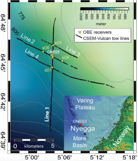
Figure 1.A map showing the CSEM survey layout along the CNE03 pockmark. Eight UoS OBEs deployed around the CNE03 pockmark. Survey lines 1–4 were conducted above the OBEs, using the DASI transmitter and the Vulcan receiver. Bottom right map: the location of the Nyegga region, bounded by the Vøring plateau and Møre basin.

is characterized by a sharp decrease in seismic amplitude, resulting from either the presence of shallow carbonate, free gas bubbles within fractures or accumulations of hydrate (Riedelet al.2002). In most cases, hydrates have no distinctive seismic reflectivity signa- ture from within the hydrate zone. Therefore seismic reflection data alone are insufficient for the quantification of gas hydrate deposits (Edwards1997; Weitemeyeret al.2011). Similar to ice, methane hydrates are electrically resistive (Edwards1997) compared to seawater and, thus, detectable by electromagnetic (EM) methods when occupying sediment pore space. The marine controlled-source electromagnetic (CSEM) technique has proven to be a promising geophysical method for the detection and evaluation of gas hydrate reservoirs (Schwalenberget al.2005; Weitemeyeret al.2011). Co- incident interpretation of seismic and electromagnetic data may allow us to distinguish between high resistivity with highP-wave velocity anomaly (hydrates) and high resistivity with lowP-wave velocity anomaly (free gas).

Offshore mid-Norway, the Nyegga region is known to accommodate about 415 pockmarks (Hustoft et al. 2010), presenting a broad range of bathymetric variations that are viable habitats for faunal communities (Hovland & Svensen2006; Paull et al.

2008; Ivanovet al.2010). The chimney and pipe structures beneath these pockmarks are estimated to contain a mean value of 710 GSm³ (GSm³ =10⁹ standard cubic metres; 85 trillion cubic

feet; equivalent to 15 million barrels of oil) of gas hydrates, that is spread over a broad region; with a resource density in the range of 0.08 GSm³km⁻²to 0.64 GSm³km⁻²(Sengeret al.2010). From the reasons mentioned above, the Nyegga region was chosen for this particular study.

In 2012, we performed a CSEM survey at one of Nyegga’s pockmarks, named CNE03 (Fig.1). The purpose of this study is to delineate both the gas hydrate and free gas reservoirs within and below the pipe structure that lies beneath this pockmark. Here we present the resistivity structure beneath CNE03 derived from 2.5-D CSEM unconstrained, seismically constrained and synthetic inversions in order to interpret this structure in conjunction with high-resolution 3-D seismic tomography from previous work by Plaza-Faverola et al.(2010,2012). This paper offers a qualitative interpretation of the results and will be followed by a second paper that will focus on quantitative analysis, using rock physics measurements of core samples from CNE03 and joint elastic-electrical models to determine the gas hydrate saturation at this pipe structure.

2 G E O L O G I C A L S E T T I N G

The Nyegga region is situated at 64^◦N, 5^◦E along the mid- Norwegian continental margin (Fig. 1) in water depths of

(3)

700–800 m, with a regional seabed slope of 1^◦ (Hovland et al.

2005; Plaza-Faverolaet al.2010). Nyegga lies at the northern flank of the Storegga slide, in the southeast part of the Vøring Plateau at the border between the Vøring and Møre sedimentary basins (B¨unz et al. 2003; Brekke2000). This area was formed by a series of rifting episodes that began in the Late Jurassic / Early Cretaceous around the Vøring and Møre basins, which led to a continental break-up by the Late Palaeocene / Early Eocene (Brekke2000).

Glacial-interglacial climate cycles have predominately shaped the depositional environment of this continental margin (Dahlgrenet al.

2002; Kjeldstadet al.2003).

The spatial extent of the Nyegga region is 200 km²(B¨unzet al.

2003), where pockmarks resulting from fluid expulsion (Judd &

Hovland1992; Plaza-Faverolaet al.2011) were detected along the seabed (Bouriaket al.2000; B¨unzet al.2003; Hovlandet al.2005;

Hovland & Svensen2006), with varying bathymetry up to 300 m wide and 12 m deep (B¨unzet al.2003; Plaza-Faverolaet al.2012).

These pockmarks are often underlain by chimney-like or pipe structures (Berndtet al.2003) that are caused by vertical fluid movement (Bouriaket al.2000; Plaza-Faverolaet al.2011). As previously described by Andresen (2012) and Karstens & Berndt (2015), we use the term chimney-like structure for large dimension diffuse vertical seismic anomalies (that have scattered complex shape, indis- tinct vertical edges and internal architecture). We use the term pipe structure for more sharply bound vertical seismic anomalies, which present internal upward deflection of seismic reflectors. The Nyegga chimney-like and pipe structures originate at different depths and connect to the top of the Miocene / Early Pliocene Kai Formation (Sejrupet al.2005; Eidvinet al.2007) via polygonal faults (Berndt et al.2003). They may reach the seafloor or terminate within the Plio/Pleistocene Naust Formation (B¨unzet al.2003; Berndtet al.

2003).

The CNE03 pockmark features a central crater at the seafloor that is underlain by a pipe structure, assumed to accommodate high hydrate concentration (Chenet al.2011). At CNE03, free gas from deep reservoirs is inferred to migrate vertically into the gas hydrate stability zone (GHSZ) via polygonal faults and fractures (Plaza- Faverolaet al.2010) and forms hydrate in veins (Hornbachet al.

2004; Jain & Juanes2009). Additionally, water with methane in solution continues to propagate upwards, forming small amounts of hydrate and authigenic carbonate near the seafloor (Foucheret al.

2009), both of which are electrically resistive. The pipe diameter is∼200 m at the seabed and∼500 m along the inferred base of the gas hydrate stability zone (BGHSZ) at 230 mbsf (B¨unzet al.

2003; Plaza-Faverolaet al.2010). At pockmarks 10 km away from CNE03, based on core samples, hydrate was found preferentially along the bedding planes and fractures (Mazziniet al.2006; Ivanov et al.2007). It is likely that gas hydrates at CNE03 are predominantly fracture filling due to the low permeability of the glacial-interglacial muddy sediment deposits found in this region (B¨unzet al.2003;

Westbrooket al.2008; Jain & Juanes2009).

3 M E T H O D S

3.1 Marine CSEM survey

Gas hydrate targets are commonly located in the top few hundred metres below the seafloor. They are predominantly manifested by a resistivity contrast of a fewm increase compared to the background resistivity (Collettet al.1998). Consequently, the marine CSEM technique (Constable et al. 1998; Constable 2006; Key

2012) was modified to use higher transmitted frequencies and a fixed offset three-axis electric field receiver, to extend the CSEM capability to detect shallow and subtle resistivity anomalies with high resolution (Weitemeyer & Constable2010). CSEM sounding is highly sensitive to volumetric changes in resistivity (Edwards2005;

Constable2010), mainly related to pore fluid properties; therefore, it can detect robustly fluid migration pathways and quantify porosity (Harris & MacGregor2006; MacGregor & Tomlinson2014; Naif et al.2015).

Our CSEM survey was conducted using the University of Southampton (UoS) CSEM system along with the GEOMAR CSEM system. In this paper, we discuss the results derived from the raw data acquired by the UoS system. The UoS CSEM survey included three types of equipment: a deep-towed active source instrument (DASI) transmitter (Sinhaet al.1990), ocean bottom electrical field receivers (OBEs; Minshullet al.2005), and a fixed- offset towed three-axis electric field receiver (Vulcan; Weitemeyer

& Constable2010; Constableet al.2012,2016). The DASI transmitter generates an electric current dipole to create a time-varying electromagnetic field that diffuses through the seawater and the seafloor. The returning secondary EM field is then recorded by the OBEs and Vulcan instruments. In this survey DASI transmitted an 81 Ampere square wave AC output current at a frequency of 1 Hz along a 100 m horizontal electric dipole (HED), generating a source dipole moment of 10.3 kAm. DASI’s position was tracked by Posidonia, an ultrashort baseline (USBL) acoustic navigation system. An altimeter was used to monitor the altitude of DASI from the seabed. A conductivity, temperature, and depth device (CTD) provided continuous measurement of the water conductivity and DASI’s depth.

Eight OBEs recorded the horizontal electric field data at a sam- pling frequency of 125 Hz, using electrodes placed on each end of two 12 m long horizontal perpendicular dipoles. OBEs 1–6 and 8 were mounted with previously used Ag-AgCl electrodes while OBE s07 was equipped with a new set of electrodes for the purpose of testing, which resulted in unusable data and, therefore, the data were discarded. The 8 OBEs were deployed (from∼20 m altitude) on the seabed using a Posidonia acoustic release attached to the ships CTD cable. The seabed positions of OBEs s04, s05, s06 and s07 were determined by the USBL acoustic navigation system while those of OBEs 01, s02, s03 and s08 were determined by the ship navigation system (due to USBL malfunction). Four OBEs were deployed within the central zone of CNE03 (s02, s03, s04, s07- spaced from each other by∼200 m) and the other four (s01, s05, s06 and s08) were placed at 1.5 km distance from the pockmark centre (Fig.1). This particular survey layout was designed to correspond with the 3-D tomographic seismic survey layout that was previously performed at CNE03 (Westbrooket al.2008). The DASI transmitter and Vulcan (towed 300 m behind DASI’s antenna) were flown approximately 50 m above the seafloor at an average speed of 1.5 knots along 5 survey lines (Fig.1, survey line 5 not shown, only Vulcan data were acquired along that line). The interpretation of the Vulcan data set is beyond the scope of this paper, however these data were used here to correct the drift in the transmitter clock.

3.2 CSEM data processing

To assess and interpret the data in the frequency domain the time series data were processed into the frequency domain using the procedure detailed in Myer et al. (2011) and summarized here.

(4)

Table 1. A table listing the Ex and Ey dipole arms orientation. The uncertainty in dipole arms orientation is2^◦.

OBE Ex orientation Ey orientation

s01 147^◦ 237^◦

s02 132^◦ 222^◦

s03 359^◦ 89^◦

s04 276^◦ 6^◦

s05 356^◦ 86^◦

s06 38^◦ 128^◦

s08 202^◦ 292^◦

The CSEM data were fast Fourier transformed using time win- dows of 1 s to give amplitude and phase data in the frequency domain. Corrections were applied to the OBEs clock drift (<1 ms d⁻¹). The data were then stacked over 60 s intervals to increase the signal-to-noise ratio. Finally, the transmitter and receivers nav- igational information was merged with the stacked data. The navigation of DASI and the OBEs were obtained using the USBL system and ship positioning as described in Section 3.1. We applied Key & Lockwood (2010) orthogonal procrustes rotation analysis (OPRA) inversion technique to calculate the orientation of the OBE dipoles (Table1). Myeret al.(2011) processing method was customized here to account for limitations in the data that were imposed during the acquisition stage. First, a significant drift in the crystal clock of DASI led to a drift in phase. A drift rate of

∼85 ms d⁻¹was used to correct for the phase drift of the transmitter. This phase drift was determined by flattening the Vulcan phase data where there are background sediments. Second, the absolute phase was not recorded and the transmitter was switched off at the end of each survey line. Therefore, static phase offsets were cor- rected for each of the towlines as derived from a comparison of the phase data with synthetic phase derived from half-space 1-D forward models.

The recorded electric field data saturated at 10⁻⁹VA⁻¹m⁻²within a transmitter (Tx)–receiver (Rx) range of∼1 km, due to the high gain of the OBE pre-amplifier. The electric field noise floor at 1 Hz (the fundamental frequency) is approximately 10⁻¹³VA⁻¹m⁻², and the DASI signal drops below this value at a Tx–Rx range of

∼3500 m.

3.3 Uncertainty analysis and error structure

Uncertainties in CSEM data can emerge partially from measurement noise and from errors in the position and orientation of both the transmitter and receivers (Myeret al. 2012a,b). Any errors in geometry will alter and ultimately bias the derived resistivity model. Thus, a well-constrained transmitter and receiver geometry is imperative to achieve a reliable interpretation of the data (Weitemeyer & Constable2014). In this survey, the transmitter dip was not recorded, therefore, we assumed a dip of 0^◦, based on the relatively flat bathymetry in the survey area. To obtain the positions of the instruments, the USBL navigation system uses a sound velocity profile of the water column. Failing to use a sound velocity obtained from the survey area may lead to errors in positions of both the transmitter and receivers. Here, the USBL system used a uniform water velocity profile (1500 m s⁻¹) rather than a stratified one, which led to a tolerable uncertainty in DASI position (mean error of∼3.5 m). This error was calculated by comparing the USBL measured depth using constant water velocity to a calculated depth assuming stratified velocity profile. To account for uncertainties in the positions of the receivers (see Section 3.1),

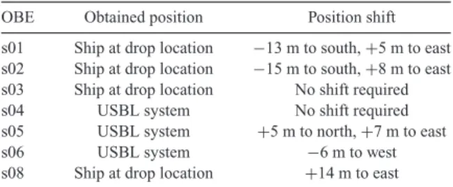
Table 2. A table listing the shift in position that were applied to the OBEs in order to achieve a symmetric distribution of the in-tow / out-tow data over the 1-D forward models.

OBE Obtained position Position shift

s01 Ship at drop location −13 m to south,+5 m to east s02 Ship at drop location −15 m to south,+8 m to east s03 Ship at drop location No shift required

s04 USBL system No shift required

s05 USBL system +5 m to north,+7 m to east

s06 USBL system −6 m to west

s08 Ship at drop location +14 m to east

we applied relative positional shifts to the OBEs as detailed in Table2. The required shifts were determined by iteratively comparing between the OBE data and synthetic electric field data derived from 1-D half-space forward models. To validate the applied OBE shifts we compared inversion results for unshifted receivers and shifted receivers and found that the applied OBE shifts insignifi- cantly alter the final model, but reduced the conductive anomalies beneath the OBEs, improved the model smoothness and lowered the final RMS.

We applied the OPRA inversion (Key & Lockwood2010) to the 1 Hz data acquired by the OBEs along survey lines 1 and 2, in order to resolve the orientations of the OBE dipole arms (Table1). The inversion required 20 iterations to fit most of the data to RMS misfit of 1.5, using an error floor of 5 per cent. When comparing between line 1 and line 2 OPRA inversions for the same OBE, the difference in orientations was in all cases2^◦.

The Occam inversion algorithm weights all data by their errors, therefore choosing a sensible error structure is almost as important as the data set itself (Constableet al.2015). Here, the inversions were assigned a fixed error structure for the amplitude, derived from the estimated geometric uncertainties and random noise error. The phase error structure was calculated using: δφ = δr/r∗180/π; whereδφrepresents the uncertainty in phase,δr is the amplitude uncertainty,ris the amplitude and the last factor converts radians to degrees (Key2009). An efficient method to estimate the error structure is by assessing the uncertainty of each position parameter using perturbation analysis (Myeret al.2012a). This analysis uses the navigated Tx and Rx geometries along with 1-D forward modelling code (Key2009) to yield a varying error structure derived from the uncertainty in data as a function of the inline / cross-line component, range and frequency. In this study, we applied a perturbation analysis to back calculate the geometric uncertainty of each Tx and Rx position parameter. This analysis indicates that the uncertainty values are: Rx orientations±2^◦, Tx dip±1^◦, Tx azimuth

±3^◦, Tx altitude±3 m, inline range±4 m, and cross-line range

±7 m. Geometry-driven uncertainties are not equal in amplitude and phase. Thus, some uncertainties may produce errors in phase that are smaller than the errors in amplitude (Myeret al.2012a).

Therefore, inverting the data decomposed into amplitude and phase is preferable to using real and imaginary parts with equal errors, which may suppress some of the accuracy available in the phase (Myeret al.2012a,b). Here, we used an average value of 4 per cent for the errors in amplitude and 2.29^◦for the errors in phase.

3.4 Properties of the 2.5-D CSEM inversion

For the 2.5-D CSEM inversions, Key & Ovall’s (2011) MARE2DEM inversion code was applied. MARE2DEM is a paral- lel goal-oriented adaptive finite element solver to compute solutions

(5)

in terms of 2.5-D models for multifrequency CSEM responses, with a high level of accuracy (Key & Ovall2011). MARE2DEM is con- ceptually based on the regularized nonlinear Occam’s inversion method (Constableet al. 1987), that seeks the smoothest model that fits the data within a specific target misfit tolerance. To balance between the model smoothness and misfit, the Occam approach utilizes a Lagrange multiplier that is an optimization parameter, updated at each inversion iteration.

Our inversion starting model included a 10¹² m air layer, 13 fixed parameters of the stratified water column with seawater resistivity values ranging between 0.2669m (at the sea surface) and 0.3389m (near the seafloor), and 1m for the subseafloor resistivity. The seawater resistivity values were derived from the conductivity data acquired by the CTD instrument (mounted on DASI). Constructing a starting model using a fine grid of finite element triangles in the shallow subseafloor, enhances the model ability to handle more complex structures and reduces the inversion total run time (Key & Ovall2011). For the subseafloor structure, we applied a finely discretized model mesh (to avoid large jumps in resistivity), with a Delaunay triangulation grid as follows: 30 m triangle size from ∼720 m to 1 km below sea-surface (the top 300 mbsf), 60 m triangle size between 1–1.5 km, 90 m triangle size between 1.5 and 2 km, 120 m triangle size between 2 and 2.5 km and 150 m triangle size from 2.5 to 3 km below sea surface.

Outside of the discretized mesh boundaries, the triangular element size increases with growing distance from the area of interest. This starting model meshing scheme resulted in 8000–13 000 free parameters, depending on the length of the towline. In this study, for the real data inversions we used a half-space model with 1m as the starting model, while for the synthetic and prejudiced inversions, we constructed variousa priorimodels that were implemented as our starting models. When the subseafloor resistivity of the starting model is much lower than that of the true model, inversion using linearly scaled data forms may lead to flat misfit curves (no mini- mization of the misfit with successive iterations due to misfit saturation), a behaviour that can prevent model convergence (Wheelock 2012). This behaviour does not happen when inverting the phase and log-scaled amplitude data since the normalized residuals will grow larger, which in turn will guide the inversion away from poorly fitting models (Key & Ovall2011). Therefore, we ran our inversions using phase and logarithmic amplitude data, which stabilize better and converge faster to a solution than inversions that uses real and imaginary components or linear amplitude and phase data (Wheelocket al.2015).

To obtain the ideal inversion model, we aimed for the lowest possible RMS target misfit while seeking for a combined criteria of model smoothness and geological plausibility. Starting from a 1m half-space model the data were inverted several times to different RMS target misfit that were between 0.5 and 1.5. We found that our preferred model is the smoothest one achieved before reaching the overfit model. Our preferred model had a target misfit of 0.9. This target misfit that is only slightly lower than the expected value of unity suggests that our error estimates were reasonably successful and, therefore, a 2-D model approximation is sufficient to fit the data (Constableet al.2015). For this paper, we ran approximately three hundred 2.5-D CSEM isotropic / anisotropic unconstrained and seismically constrained inversions, while applying various model parameterizations, to seek for the optimum inversion model parameterization for this specific data set that yielded a structurally sensible final model (Table3). We favoured solutions that produced the minimum necessary structure to fit the data, thus implementing Occam’s razor (Myeret al.2015).

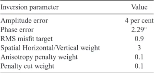
Table 3. Parametrization of the 2.5-D CSEM inversions, applied by the MARE2DEM inversion code (Key & Ovall2011).

Inversion parameter Value

Amplitude error 4 per cent

Phase error 2.29^◦

RMS misfit target 0.9

Spatial Horizontal/Vertical weight 3

Anisotropy penalty weight 0.1

Penalty cut weight 0.1

4 R E S U L T S

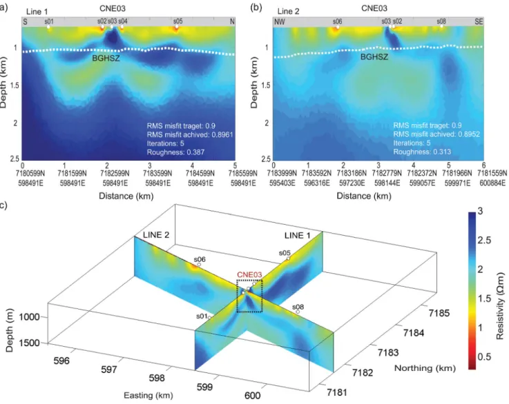
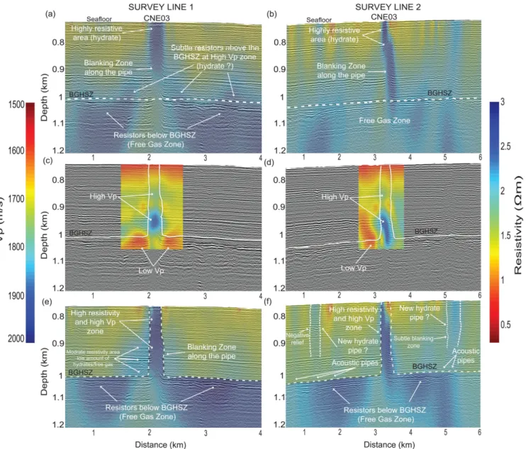
4.1 Isotropic 2.5-D CSEM unconstrained inversions The isotropic 2.5-D multifrequency (1, 3, 5, 7, 9, 11 Hz) unconstrained smooth inversion results for the south (S) to north (N) survey line 1, and northwest (NW) to southeast (SE) survey line 2 are shown in Fig.2(a). Both inversions resolved the same anomalously resistive features beneath the CNE03 pockmark. The 2.5-D inversion for line 1 shows a resistive feature of∼3m that is located between receivers s03 and s04. The ∼3m resistivity anomaly stretches from the seafloor (∼724 m below sea level) to a depth of∼270 m (∼1000 m from sea surface), within the GHSZ. This delineates a typical pipe structure, suggested to contain gas hydrate vertically beneath the location of the CNE03 pockmark (Westbrook et al.2008; Plaza-Faverolaet al.2010,2012). Below the BGHSZ, located roughly at 1.1 km depth, a∼150 m thick horizontal resistive anomaly is present (Fig.2a), which indicates free gas accumulation (Plaza-Faverolaet al.2010). The region beyond ∼1.7 km depth shows a large and laterally extensive resistor, which might be either an free gas zone (FGZ) that is the source of gas feeding the upper structure, or an artefact resulting from inversion insensitivity below this depth.

The line 2 isotropic smooth inversion (Fig.2b) shows a similar trend to that observed in line 1; a resistive pipe structure beneath CNE03 that is slightly skewed to the southeast, narrower and deeper (∼1.1 km depth) than the one present in line 1 inversion. The intersection between line 1 and line 2 adequately locates the pipe structure at CNE03, as imaged by both lines (Fig.2c). Line 1 and 2 isotropic inversions were converged to a target misfit of 0.9 after 5 iterations while producing very smooth resistivity models (low roughness values).

Shallow conductive anomalies are observed beneath the receivers as shown in Figs2(a) and (b). We do not interpret these anomalous areas as we believe they are inversion artefacts. We were unable to determine the absolute cause, however a phase only inversion did not exhibit the conductive anomaly below each OBE suggesting the is- sue is embedded in the amplitude data. Inversions with different dip, OBE shifts, and seawater resistivity all resulted in a main resistive pipe structure observed beneath the CNE03 pockmark and therefore it is a feature required by the data. To determine the horizontal and vertical sensitivity of the inversions, we ran various synthetic and prejudiced inversions, which are presented in Section 4.5.

In a CSEM unconstrained smooth inversion, subtle resistors that are unassociated with a seismic blanking zone or acoustic pipes might be the result of a smearing effect due to the diffusive nature of the EM field. Such subtle resistors are observed above the BGHSZ in line 1 unconstrained inversion (Fig.4a), that besides artefacts may also indicate low saturations of hydrate. To resolve this ambiguity and better constrain the pipe structure at CNE03, we performed seismically constrained inversions (Section 4.3), using

(6)

Figure 2. (a) Line 1 unconstrained smooth isotropic inversion. (b) Line 2 unconstrained smooth isotropic inversion. The circles represent OBE sites. The inferred depth of the BGHSZ situated slightly under 1 km below sea surface taken from Plaza-Faverolaet al.(2010). (c) Fence diagram showing inversion results for towlines 1 and 2. The CNE03 pipe structure observed at the towlines intersection. Towline 2 southeast shallow resistor is likely to be interlink with the deeper resistor below the BGHSZ.

both the seismic reflection data and a smooth Vp model that we constructed (Section 4.2) using Plaza-Faverolaet al.(2010) layered Vp model.

4.2 3-D seismic tomography

Resistivity anomalies due to hydrate and free gas in a pockmark pipe structure can be distinguished by considering the seismic velocity contrast between the high-velocity zone (HVZ) due to hydrate and the low-velocity zone (LVZ) due to gas, where the HVZ–LVZ boundary is indicative to the BGHSZ location. Traveltime tomography seeks to resolve the subsurface velocity model that best satisfies the traveltimes of seismic waves that propagate through the subsurface (Plaza-Faverolaet al.2010). The layered Vp model for the CNE03 pockmark (Plaza-Faverolaet al.2010) was created using TomoInv, a pre-stack traveltime tomography software, developed at Institut Franc¸ais du P´etrole (Delboset al.2001,2006).

Here we present two representations of the CNE03 pockmark Vp model, the original layered representation and a smoothed version (Fig.3). We show planar slices through the velocity model that

correspond to the cross-lines (line 1 and 2) of the CSEM survey.

The smoothed version was built using a Gaussian filter with an effective filter width of∼5 m in thex/y-direction and∼50 m in thez-direction. The dimensions of this particular filter were chosen by gradually increasing the smoothing scale until minimal discontinuity between the layers was achieved. Both Vp representations start at the seafloor (∼727 m below sea-surface) and extend to a depth of 1000 m (line 1, S to N) and 1050 m (line 2, NW to SE), below sea-surface. The velocities in the first and the second layer (727–750 m, and 750–800 m) are poorly constrained at the pipe structure interior and its flanks, due to a low density of seismic- ray impact points in this region (Plaza-Faverolaet al.2010). The model shows an increased seismic velocity along the pipe structure compared with the surrounding strata, most probably resulting from the presence of hydrate in the pores of the host sediments within the GHSZ (Figs3a and c). In the line 1 Vp model at∼1000 m, a decrease in seismic velocity is observed (Figs3a and b) that co- incides with the location of the inferred BGHSZ. This decrease in P-wave velocity is attributed to a free gas layer that lies below the BGHSZ. In the line 2 Vp model (Figs3c and d), the highest velocity

(7)

Figure 3.Vp models of the CNE03 chimney structure. (a,b) Layered and smooth Vp models of line 1. (c,d) Layered and smooth Vp models of line 2. (e) A fence diagram showing smooth Vp model of line 1, line 2 and the BGHSZ horizon. The tomographic inversion was implemented using data from both single channel seismic (SCS) and 16 ocean bottom seismic (OBS) recorders (Plaza-Faverolaet al.2010).

region is elongated, extends deeper than the equivalent zone in line 1 and is slightly tilted towards the east, which is consistent with the pipe resistivity anomaly at CNE03, as shown in Fig.2(b). The high Vp regions of both lines are located beneath the CNE03 pockmark (Fig.3e). East of CNE03 high velocities exist immediately above the BGHSZ, whereas low velocities appear west of CNE03 (Fig.3e).

4.3 Seismically constrained 2.5-D CSEM inversions Our isotropic CSEM unconstrained inversion results, for both line 1 and line 2 co-rendered with the corresponding seismic reflec-

tion sections, present a reasonable fit between the seismic blanking zone of the CNE03 pipe structure and the vertical resistive anomaly (Figs4a and b). To improve the unconstrained inversion results for line 1 and line 2, we constrained them with seismic information. In a seismically constrained CSEM inversion, the structural smoothing regularization enables any seismically derived stratigraphic attribute to constrain the EM data, thus yielding a refined and geologically realistic final model (Wiiket al. 2015). In our seismically constrained inversions, the regularization is relaxed across seismically defined interfaces, thus enabling a discontinuity to appear if one is favoured by the data. Our seismic constraint scheme here is primar- ily based on the seismic reflection data and supported by the 3-D

(8)

Figure 4.A comparison between unconstrained and seismically constrained 2-D CSEM inversion. Both the unconstrained and constrained inversions are co–rendered with the corresponding seismic reflection sections. (a,b) Lines 1 and 2 unconstrained inversions. (c,d) Vp models of lines 1 and 2, the area within the white lines, represent the constrained region applied in the seismically constrained inversions. (e,f) Lines 1 and 2 seismically constrained inversions. To acquire the seismic reflection sections, a GI-gun source and a seismic streamer with three 25 m long active parts (carrying 37 hydrophones per section at a spacing of 0.6 m) were used (Westbrooket al.2008).

seismic tomography. The seismic reflection sections were acquired using a mini-GI-gun and a two-channel seismic streamer (Exley &

Westbrook2006; Westbrooket al.2008).

4.3.1 CNE03 pipe structure delineation

The upper pipe structure of CNE03 was constrained using the seismic reflection data, by tracing the vertical blanking zone slightly beyond the pull-up reflections (Figs4c and d). The lower part of the pipe structure below 820 m depth was constrained horizontally by the vertical boundaries of the blanking zone and the coincident highP-wave velocity in that zone which supports the presence of hydrates. The CSEM inversions were constrained also across the inferred BGHSZ horizon, as shown in Figs4(c) and (d). These constrained inversions successfully aligned the vertical resistivity anomalies with the columnar seismic blanking zone (Figs4e and

f). The line 1 constrained inversion shows that the pipe structure boundaries properly confine the anomaly that stretches continuously from the seafloor to the BGHSZ (Fig.4e). This result contrasts with the unconstrained inversion where the anomaly magnitude de- creases at∼900 m (Fig.4a), and the Vp model where anomalously high velocities start to appear only from∼100 mbsf (Fig.3b). The pipe structure is∼200 m wide and∼290 m in vertical length. Re- sistivity features above and below the BGHSZ were significantly decoupled by the constrained inversion, as seen by the sharp contrast in resistivity across the BGHSZ. This decoupling suggests that the subtle resistors observed above the BGHSZ in line 1 unconstrained inversion are more likely to be artefacts caused by the inversion smoothing rather than hydrate deposits. However, in the constrained inversion a moderate resistor remained in the area located between the BGHSZ and the outer southern part of the pipe structure (Fig.4e). To determine if this resistive area is an artefact or a real geological feature, we applied a forward model based on

(9)

line 1 constrained inversion final model. In this forward model the resistive region deep beneath OBE s02 between the pipe structure and the BGHSZ, were assigned with the background resistivity. This forward model significantly degraded the model fit to the amplitude data and correspondingly increased the residuals. This result suggests that the moderate resistive area is a real geological feature, most likely representing a low concentration of hydrate or free gas.

From a comparison between line 1 unconstrained and constrained inversions, no change is observed in the distribution of the resistive anomalies along the FGZ, though both the pipe structure resistor and the FGZ resistor present higher resistivity values in the constrained inversion (Figs 4a and e). The line 2 unconstrained and constrained CSEM inversions both show two vertical anomalies that extend from the seafloor to a depth of about 940 mbsf, one at a distance of∼1.2 km (NW) and a second at∼5.3 km (SE), as seen in Fig. 4(f). Both anomalies coincide with several acoustic pipes and subtle blanking zones. These subtle resistors may indicate the presence of pre-existing fluid pathways or new emerging ones that have yet to be manifested as pockmarks. In the constrained inversion, the pipe structure resistive anomaly is well bounded by the columnar seismic blanking zone, though still slightly tilted from NW to SE (Fig.4f). The resistors in the FGZ, are more extensive than the resistors observed in the unconstrained inversion (Figs4b and f).

4.3.2 Model to data fit

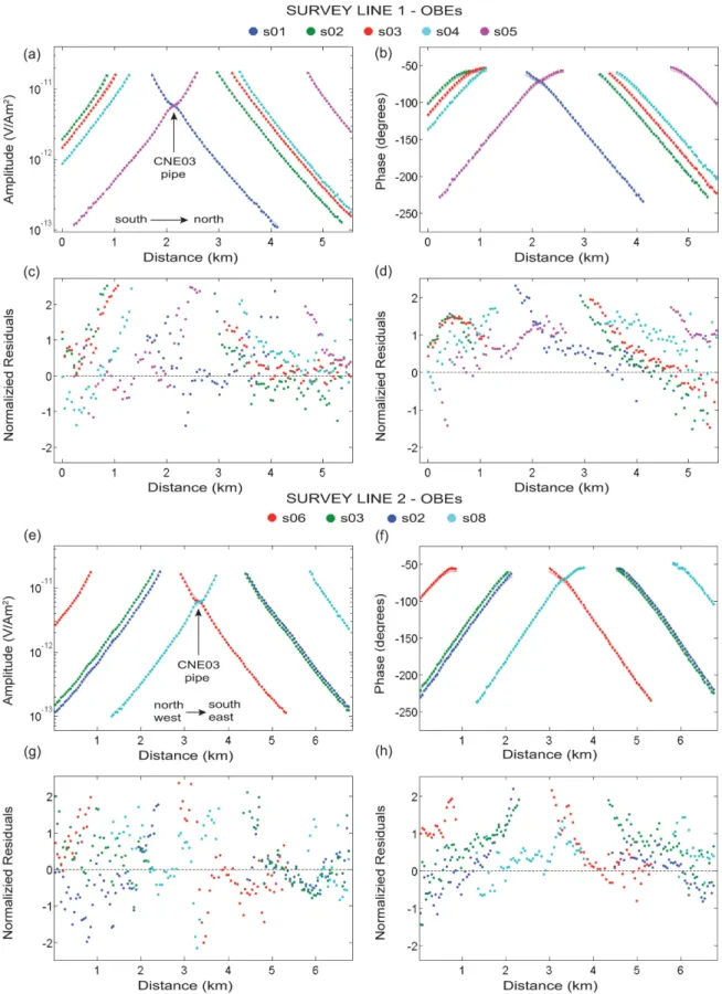
The same model parameterization (Table3) was applied for both the unconstrained and seismically constrained inversions. As for the unconstrained inversions, the seismically constrained inversions converged as well to a target misfit of 0.9. OBEs s01 and s05 in survey line 1, as well as s06 and s08 in survey line 2, show a subtle increase in amplitude at a Tx–Rx offset of ∼1.5 km. These ele- vations in amplitude intersect at the exact location of the CNE03 pockmark, thus representing the underlying pipe structure resistivity anomaly (Figs5a and e). For these seismically constrained inversions, the fits between the 2-D model and the amplitude and phase data at the fundamental frequency of 1 Hz are shown in Fig.5.

All OBEs achieved a reasonably good model to data fit in both amplitude and phase (Figs5a,b,e and f), though the 1 Hz normalized residuals systematically increase at short offsets (Figs5c,d,g and h).

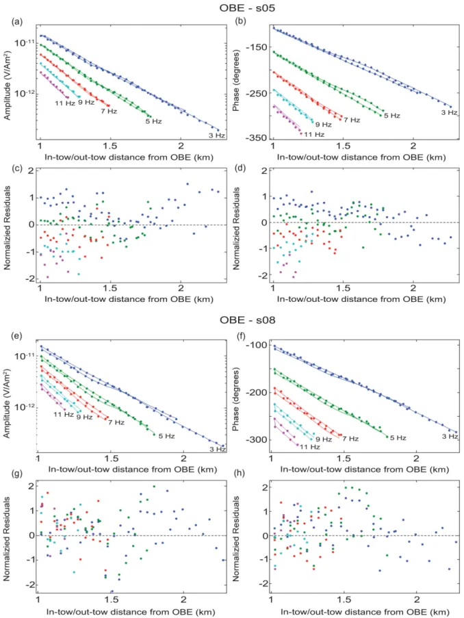
The asymmetric structure in the 1 Hz data residuals suggests it may all be due to transmitter dip, which was not measured. An inversion with a transmitter dip of 5^◦eliminated some of the residuals structure at the short offsets, but did not eliminate the shallow conductive anomalies beneath each receiver. Furthermore, the final model did not change significantly. This is because errors in navigation are accounted for in our uncertainty analysis and error budget. The bias in residuals is within the bounds of the error structure for both the amplitude (4 per cent) and phase (2.29^◦). At higher frequencies the normalized residuals are smaller and unstructured, as shown in Fig.6for OBEs s05 and s08 (all other OBEs presented similar trend). Therefore, the overall data to model fit are satisfactory.

4.4 Anisotropy at CNE03

Thin-layer horizontal sediment grain alignment would most likely result in electrical anisotropy (Ramananjaona & MacGregor2010).

Seismic anisotropy may also exist in regions where vertical to sub- vertical, fluid-filled fractures and micro-cracks are present (Exley et al. 2010). The Nyegga pockmarks region exhibits a subhori-

zontal stratigraphy (Kjeldstad et al. 2003) as seen from extensive seismic reflection data (B¨unzet al.2003; Berndtet al.2003;

Westbrooket al.2008; Plaza-Faverolaet al.2010,2011). The underlying chimney-like and pipe structures cut vertically through the horizontal layers (B¨unzet al.2003; Berndtet al.2003; Plaza- Faverolaet al. 2011). The geological setting and the presence of upwardly migrating free gas via vertical structures, both increase the probability for anisotropy at CNE03. Electrical anisotropy is commonly defined as the ratio between the vertical resistivity and the horizontal resistivity while a ratio above 1.5 indicates the exis- tence of significant anisotropy (Werthm¨ulleret al.2014). Analysing anisotropic structure by applying isotropic CSEM inversion may provide biased results that are inconsistent with other data sets such as seismic and well logging (Ramananjaona & MacGregor2010).

Therefore, accounting for anisotropic effects may be necessary to accurately describe a given earth structure by a resistivity model.

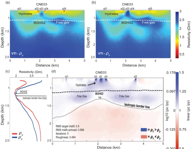
Here, we applied a vertical transverse isotropic (VTI) multifrequency (1, 3, 5, 7, 9 and 11 Hz) CSEM inversion for the data acquired from survey line 1 (Fig.7). VTI is also known as TIZ—transversely isotropic perpendicular to thez-axis (ρx= ρy =ρz, whereρ is resistivity), which is one form of the conductivity tensor that represents anisotropy (Key & Ovall2011). Spatial variations in our model were penalized (3:1 bias against horizontal versus vertical variation) and the penalty for anisotropy was reduced from 1 to 0.1 as part of the inversion regularization, thus, enabling the inversion to better resolve anisotropic anomalies. The conductive anomalies observed below the receivers in the isotropic models, diminished significantly in the anisotropic vertical resistivity model (Fig.7b).

Thus, the anisotropic model offers a slightly better fit to data. This result supports the notion that a moderate level of anisotropy is present in the first layer of sediments below the receivers. The vertical resistivity model (ρz) shows the shallow anomalous resistors as well as the deeper resistor slightly better than the horizontal resistivity model (ρy) which resolve poorly the resistivity at the pipe structure and along the BGHSZ beneath s01 and s02 (Figs7a and b).

The anisotropy ratioρz/ρyshows that the vertical resistivity is about 1–1.2 times greater than the horizontal resistivity beneath CNE03 and along the BGHSZ region. From∼1.3 km downward,ρz/ρyra- tio changes such thatρybecomes roughly 1–1.1 times greater than ρz(Figs7c and d).

4.5 Sensitivity analysis using synthetic and prejudiced inversions

In synthetic model studies where the true model is known, the inversion algorithms and survey parameters can be examined for their capability to resolve the true EM structure (Constableet al.

2015; Tsenget al. 2015). To produce reliable synthetic models, pragmatically it is advisable to introduce simple structures within a homogenous host (Constableet al.2015). Here, we conducted numerous synthetic studies aiming to describe the sensitivity and resolution of the 2.5-D inversion to the real data, and to reveal any false positive resistivity features that are artefacts introduced by the survey layout or the inversion process. Our synthetic data sets were constructed using the same frequencies, geometric configuration, data coverage, source navigation and receiver position that were applied to invert survey line 1 real data. We added Gaussian noise to the synthetic data sets equal to the error structure used for inverting the real data (Table3).

As observed in both the unconstrained and constrained inversions (Figs2and4), the resistivity anomaly at CNE03 is 1–1.5m,

(10)

Figure 5.Lines 1 and line 2 seismically constrained inversions model to data fits: showing the electric field amplitude and phase data at 1 Hz, with their corresponding normalized residuals. The dots represent the data, lines represent the 2-D model responses and the vertical bars are data uncertainties. All OBE receivers present similarly adequate fit between the 2-D model and the data.

(11)

Figure 6. OBE s05 (line 1) and OBE s08 (line 2) model to data fits from the seismically constrained inversions, showing the electric field amplitude and phase data for 3, 5, 7, 9, and 11 Hz, with their corresponding normalized residuals. The dots represent the data, lines the 2-D model responses and the vertical bars are data uncertainties. Adequate fit between the 2-D model and the data is observed at all frequencies.

(12)

Figure 7.Survey line 1 CSEM anisotropic inversion. (a) Horizontal resistivity, (b) vertical resistivity, (d) vertical to horizontal resistivity ratio (ρz/ρy). The ρz/ρyratio presented in both linear and log10scales. The circles represent OBE sites. The blue colour represents the areas whereρz> ρyand the red colour shows the areas of whichρz< ρy. The white colour represents isotropic regions. (c) A comparison betweenρy(red line) andρz(blue line) vertical profiles.

The profiles extracted from the centre of the pipe structure, horizontally at 2.16 km. Areas where the profiles overlap represent isotropy.

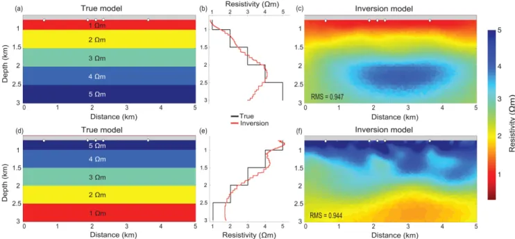
which is a factor of∼2, above the background resistivity of the host sediments. Therefore to assess the inversion resolution for this particular resistive anomaly, we tested layered synthetic models (resistive to conductive and vice versa) with fine increments of only 1m every 500 m (apart from the first∼250 m layer) extending from the seafloor to a depth of 3 km, as presented in Fig.8. In the case of the conductive to resistive layered synthetic model (Fig.8a), the inversion successfully differentiated between the layers up to a depth of∼2.5 km, with high sensitivity both vertically and horizontally (Fig.8c). The recovery of the last detectable layer (4m) is mostly satisfactory, while horizontally the inversion is mainly sensitive to the area between∼1.7–3.7 km along the survey line. The inversion was not able to resolve the lowest 5m layer (Fig.8b).

The resistive to conductive layered model (Figs8d–f) resulted in a laterally varying inversion model though the general layering trend was resolved by the inversion with only subtle vertical shifts. The deepest layer (2.5–3 km depth) remained unresolved (Figs8e and f), while the lowest resolved resistivity is∼1.6m, located horizontally between∼1.5–3.7 km. From these synthetic models we conclude that, for this particular data set, the inversion is sensitive to depths from the seafloor to∼2.5 km and horizontally sensitive

from∼1.5–3.7 km along the survey line. Therefore, we only interpret resistivity structures that emerged from the data inversions within this region.

To test the vertical sensitivity inferred by the synthetic models, we inverted line 1 real data with an addition of a ‘prejudice’ conductive (250 m in thickness) layer positioned between 1.5 and 3 km in six successive isotropic inversions (Fig.9). In a prejudiced inversion, any deviation from ana prioribackground value is penalized. Here, the penalty weight for the prejudice conductive layer was set to 1.0. In these inversions, our primary assumption is that when the conductive layer that we forced upon the model is positioned deeper than the maximum depth of sensitivity, we expect to get a final model that is not affected by the presence of this prejudiced layer. Hence, a final inversion model that is similar to the real data model both in structure and model to data fit. When positioned successively at depths between 1.5 and 2.25 km, the conductive layer strongly affects the final model, as implied by the observed oscillatory model and artefact features (Figs9a–c) compared to the smooth inversion final model (Fig.2a). No significant changes are observed in the resistivity structure for the three inversions where positioning the conductive layer at 2.25–3 km depth (Figs 9d–f). In the last two

(13)

Figure 8. Layered synthetic model studies that utilize the geometry, data range and properties of survey line 1. (a) Synthetic layered conductive to resistive forward model. (b) Vertical resistivity profiles that compare between the true (black line) and inversion (red line) models of the conductive to resistive synthetic test. The resistivity versus depth profiles extracted at a horizontal distance of 3 km. (c) Inversion model of the synthetic data from the conductive to resistive forward model. (d) Synthetic layered resistive to conductive forward model. (e) Vertical resistivity profiles that compare between the true (black line) and inversion (red line) models of the resistive to conductive synthetic test. The resistivity versus depth profiles extracted at a horizontal distance of 3 km.

(f) Inversion model of the synthetic data from the resistive to conductive forward model. The circles represent OBE sites.

Figure 9.Line 1 real data CSEM isotropic inversions, with an addition of a 250 m thick conductive horizontal layer, positioned at successive depths, ranging from (a) 1.5 km to (f) 3 km. The prejudiced conductive layer affects the inversion model when located between 1.5 and 2.5 km. Below 2.5 km, the conductive layer no longer alters the final inversion model. The circles represent OBE sites. The RMS target misfit to all models is 0.9.

inversions (Figs9e and f) the models fits the data just as well as in the smooth inversions. Thus, we deduce that the inversion has no sensitivity to features that are deeper than∼2.5 km, the depth at which the prejudiced conductive layer no longer alters the final inversion model.

Next, we performed a series of synthetic inversions in which resistivity structures observed in line 1 real data inversion were added successively. These synthetic tests were specifically designed to (1) distinguish which structures are real and which are artefacts;

and (2) estimate the depth, thickness and extent of the resistor

(14)

that gave rise to the lateral resistivity structure (free gas layer) below the BGHSZ (Fig.2a). First, to mimic the upper resistivity structure seen in the real data inversion, a synthetic model was constructed containing a 3m pipe structure embedded in 1.6m horizontal layer and a background resistivity of 2m (Fig.10a).

The inversion model successfully resolved the synthetic features, though also added two subtle artefacts (conductive and resistive) beneath the true upper structure (Fig.10b). Second, to the synthetic model seen in Fig.10(a), we added a 3m horizontal layer that merges with the primary pipe structure (Fig. 10c) to mimic the entire upper structure as seen in the real data inversion (Fig.2a).

Once again, the synthetic inversion adequately resolved the whole upper structure and added two conductive features at ∼1.5 km (Fig.10d) that were also observed in the real data inversion at these particular locations. Therefore, we infer that these features are artefacts possibly resulting from the inversion smoothing process rather than real subseafloor structures. Finally, to characterize the free gas layer below the BGHSZ, we alternately added a 3 m (250 m thick) horizontal resistor at depths 1.75–2.75 km (Figs10e, g, i and k). Only the inversions in which the resistor position was at depths 1.75–2 km and 2–2.25 km produced an extensive lateral resistivity structure (Figs10f and h), similar to the one observed in the real data inversion (Fig.2a). If the actual position of the free gas layer is deeper than∼2.5 km, it would have been undetectable by the real data inversion (beyond the depth sensitivity), as shown by the synthetic inversion in Fig.10(l). Therefore, we propose that the free gas layer that lies beneath CNE03 is about 250 m thick, located between∼1.75–2.25 km depth and extends horizontally further than the horizontal inversion sensitivity (>2 km), which is governed by receiver spacing and survey design.

5 D I S C U S S I O N

5.1 The potential of CSEM data to detect gas hydrate provinces

CSEM inversion methodologies are inherently non-unique due to the diffusive nature of the electromagnetic field. Such non- uniqueness may lead to interpretation ambiguity that can be miti- gated adequately by integrating all available geophysical data for the purpose of forward, inverse and synthetic modelling (Tseng et al.2015). Our 2.5-D CSEM inversions were proven to be effective in detecting resistivity anomalies in the pockmark region.

However, these inversions might present biased results due to their limited lateral and vertical sensitivity and possible artefacts. Here, we demonstrated that by using various synthetic inversions we were able to determine both the horizontal and depth sensitivity of the inversions, as well as distinguish between real resistive anomalies and those that are artefacts which appear beneath the CNE03 pockmark. The magnitude of the main resistivity anomaly (>3m) beneath CNE03 that emerged from our inversions is consistent with the magnitudes found in other gas hydrate exploration studies (Schwalenberget al.2005,2010; Weitemeyeret al.2011; Sun et al.2012). The data here presented moderate sensitivity to the presence of anisotropy at CNE03 though using EM data solely to determine the level of anisotropy present in the real subseafloor structure is a challenging task (Constableet al.2015). Therefore, since anisotropy is not essential in order for the model to fit the data, we infer that isotropic inversions are sufficient to describe the resistivity structure that lies beneath the pockmark. Both the CSEM and the seismic data sets indicated the same pipe structure anomaly

at CNE03, which strongly verifies the presence of hydrates at this location. The seismically constrained inversions successfully delin- eated the structural boundaries of the resistive pipe and the free gas layer beneath the BGHSZ.

5.2 Geological implications

The strongest resistivity anomalies observed at the shallow part below the pockmark within the pipe structure suggest the presence of authigenic carbonates or gas hydrate. Chemical analysis of core samples from the G11 pockmark (nearby CNE03) suggests that seafloor authigenic carbonates are gas hydrate origin (Mazziniet al.

2006); while gravity cores obtained from several Nyegga pockmarks (CNE03, Sharic, Bobic, Tobic and G1l) displayed distinctive signs of gas hydrate in the sediment (Ivanovet al.2007). Therefore, we suggest that the subseafloor high-resistivity anomalies observed in our inversion models represents the accumulation of hydrate rather than carbonates. We infer that the saturation of hydrate is higher in this upper region than elsewhere along the pipe structure and at the BGHSZ. High hydrate saturation at that location is probably due to preferential gas advection and interaction of the gas hydrate stability field with the free gas (Flemingset al.2003; Liu & Flemings 2007; Smithet al.2014). While high resistivities can result from both free gas and gas hydrate, high seismic velocities can only be caused by gas hydrate. Therefore, the high velocities observed at the pipe centre (∼820–1050 m) that coincide with relatively high resistivities, are indicative of high hydrate saturation at these depths. Westbrooket al.(2008) suggested hydrate saturation of up to 35 per cent within the CNE03 pipe structure, while based on a more detailed analysis, Plaza-Faverolaet al.(2010) proposed a saturation range between 14 to 27 per cent.

Archie’s Law (Archie1942) is a commonly used method for the interpretation of electrical resistivity (Ellis2008). Using a re- lationship based on Archie’s equation (eq. 1), the formation bulk resistivity of any geological feature could be related to the hydrocarbon concentration,

ρb=aϕ⁻^mS_w⁻ⁿρw. (1) In this equation,ρb represents the in situ formation bulk resistivity, ρwis the formation pore water resistivity andS_w is the pore water saturation. Here, we applied Archie’s equation to obtain a preliminary estimation of gas hydrates saturation along the CNE03 pockmark. For this calculation we used a porosity (ϕ) of 60 per cent from Hustoftet al.(2009), a formation pore water resistivity of 0.325m, and a bulk resistivity value of 3m from the 2-D unconstrained inversion. Based on the analysis of Hyndmanet al.(1999), we used a tortuosity coefficienta =1.40, a cementation coeffi- cientm=1.76, and a saturation exponentn=2. According to our Archie’s Law calculation, the CNE03 pipe structure has a hydrate concentration of approximately 38 per cent. At Vestnesa Ridge, West Svalbard margin (∼1500 km north–northeast to Nyegga), a pockmark with similar characteristics to CNE03 is present. Based on a similar analysis, the Vestnesa Ridge pockmark is estimated to have a hydrate saturation of 52–73 per cent within the upper part of the chimney-like structure (Goswamiet al.2015).

At CNE03, there is a discrepancy between the resistivity anomalies that begin at the seabed surface and extend all the way to the BGHSZ via the pipe structure and the Vp anomalies that only start from∼100 m below the surface. This discrepancy may be attributed to an artefact in the seismic tomography, caused by the low density of reflection points (Plaza-Faverolaet al.2010). Consequently,

(15)

Figure 10.A series of synthetic inversions, based on the characteristics of survey line 1. Resistive features observed in the real data inversion consecutively added to the synthetic forward model. Left column: synthetic forward models. Right column: inversion models of the synthetic data from the forward models.

The circles represent OBE sites. The RMS target misfit to all models is 0.9.

(16)

our resistivity model is likely to better represent the distribution of hydrates in the upper part of the pipe structure than the Vp model.

A low anisotropy ratio was derived from our anisotropic inversion, suggesting that only a moderate anisotropy may exist beneath the CNE03 pockmark. We propose that in regions where the horizontal resistivity is greater than the vertical resistivity (1.5 km depth), a vertical structure is present that accommodates a high density of fractures. This vertical structure acts as a pathway for an upward migration of free gas into the GHSZ, where methane hydrate forms in veins. Linked vertical hydrofractures and micro- cracks, may provide vertical flow pathways for methane-rich fluids (Mazziniet al.2003). Such vertical flow could decrease the pore pressure and may induce localized stress rotations around the gov- erning regional fault (Wright & Weijers2001; Zoback2010). Thus, we propose that the tilted nature of the CNE03 pipe structure towards SE might be a result of the local stress regime, subjected to changes in fluid flux and direction of the underlying fault, vertical fractures, and fluid flow at CNE03.

6 C O N C L U S I O N S

To estimate reliably the amount of hydrate that occupies submarine pipe structures on a global scale, a rigorous characterization of these hydrate systems is required. The CSEM method offers a new and independent tool to detect, delineate and quantify hydrate provinces due to its sensitivity to pore fluid properties. The results of this study indicate the following:

(1) The CNE03 pipe structure is approximately 200 m wide and 290 m long, as derived from our seismically constrained CSEM inversions.

(2) The3m resistivity anomaly that exist both at the pipe structure and below the BGHSZ, along with the Vp contrast across the BGHSZ, confirm that hydrates predominantly occupy the sediment’s pore space within the pipe above the BGHSZ, while free gas dominates the region below the BGHSZ.

(3) The CNE03 pipe structure is tilted towards the SE, possibly due to rotation of the minimum stress direction away from horizontal.

(4) The synthetic studies revealed two artefact features (conductive anomalies) beneath the BGHSZ, and determined the width (∼2 km) and depth (∼2.5 km) of the region to which the inversion is sensitive. Furthermore, these studies highlighted the thickness (∼250 m) depth range (∼1.75–2.25 km) and horizontal extension (2 km) of free gas accumulation beneath CNE03.

In light of the above, we conclude that our joint interpretation of the CSEM and seismic data sets were able to detect and robustly delineate both the methane hydrate and free gas deposits at the CNE03 pockmark, with a high level of accuracy.

A C K N O W L E D G E M E N T S

This paper forms part of the PhD studies of Eric Attias, who was funded by Rock Solid Images Ltd, the University of Southamp- ton, and the National Oceanography Centre (NOC). The German Research Council funded the research cruise. OBE receivers were operated by the UK Ocean Bottom Instrumentation Consortium.

TAM was supported by a Wolfson Research Merit Award. The authors would like to thank Kerry Key for providing the MARE2DEM inversion code, David Myer for the processing codes, Andreia Plaza- Faverola for the seismic velocity model, Graham Westbrook for the

bathymetric data and Christian Buckingham for helpful discussions.

Additionally, we thank Laurence North, H´ector Mar´ın-Moreno and Yee Yuan Tan, for operating the UoS CSEM system, and the captain, crew and scientific party of Meteor Cruise M87/2 COSY.

R E F E R E N C E S

Andresen, K.J., 2012. Fluid flow features in hydrocarbon plumbing systems:

what do they tell us about the basin evolution?,Mar. Geol.,332,89–108.

Archer, D., 2007. Methane hydrate stability and anthropogenic climate change,Biogeosci. Discuss.,4(2), 993–1057.

Archer, D., Buffett, B. & Brovkin, V., 2009. Ocean methane hydrates as a slow tipping point in the global carbon cycle,Proc. Natl. Acad. Sci., 106(49), 20 596–20 601.

Archie, G., 1942. The electrical resistivity log as an aid in determining some reservoir characteristics,I. Pet Tech,5,doi:10.2118/942054-G.

Berndt, C., B¨unz, S. & Mienert, J., 2003. Polygonal fault systems on the mid-Norwegian margin: a long-term source for fluid flow,Geological Society, London, Special Publications,216(1), 283–290.

Boswell, R. & Collett, T.S., 2011. Current perspectives on gas hydrate resources,Energy Environ. Sci.,4(4), 1206–1215.

Boswell, R.et al., 2015. Prospecting for marine gas hydrate resources, Interpretation,4(1), SA13–SA24.

Bouriak, S., Vanneste, M. & Saoutkine, A., 2000. Inferred gas hydrates and clay diapirs near the Storegga Slide on the southern edge of the Vøring Plateau, offshore Norway,Mar. Geol.,163(1), 125–148.

Brekke, H., 2000. The tectonic evolution of the Norwegian Sea Continental Margin with emphasis on the Vøring and Møre Basins,Dyn. Norwegian Margin,167,327–378.

Buffett, B. & Archer, D., 2004. Global inventory of methane clathrate:

sensitivity to changes in the deep ocean,Earth planet. Sci. Lett.,227(3), 185–199.

B¨unz, S., Mienert, J. & Berndt, C., 2003. Geological controls on the Storegga gas-hydrate system of the mid-Norwegian continental margin, Earth planet. Sci. Lett.,209(3–4), 291–307.

Chen, Y., Bian, Y., Haflidason, H. & Matsumoto, R., 2011. Present and past methane seepage in pockmark CN03, Nyegga, offshore mid-Norway, in Proceedings of the 7th International Conference on Gas Hydrates, (ICGH 2011), 17-21 July 2011, Edinburgh,ICGH 2011, Edinburgh.

Collett, T.S.et al., 1998. Well log evaluation of gas hydrate saturations, in SPWLA 39th Annual Logging Symposium,pp. 1–14, Society of Petro- physicists and Well-Log Analysts.

Constable, S., 2006. Marine electromagnetic methods: A new tool for offshore exploration,Leading Edge,25(4), 438–444.

Constable, S., 2010. Ten years of marine CSEM for hydrocarbon exploration, Geophysics,75(5), 75A67–75A81.

Constable, S., Kannberg, P., Callaway, K. & Mejia, D.R., 2012. Mapping shallow geological structure with towed marine CSEM receivers: 82nd annual international meeting, SEG,Expanded Abstracts,10,1190.

Constable, S., Orange, A. & Key, K., 2015. And the geophysicist replied:

‘Which model do you want?’,Geophysics,80(3), E197–E212.

Constable, S., Kannberg, P.K. & Weitemeyer, K., 2016. Vul- can: A deep-towed csem receiver, Geochem. Geophys. Geosyst., doi:10.1002/2015GC006174.

Constable, S.C., Parker, R.L. & Constable, C.G., 1987. Occam’s inversion:

A practical algorithm for generating smooth models from electromagnetic sounding data,Geophysics,52(3), 289–300.

Constable, S.C., Orange, A.S., Hoversten, G.M. & Morrison, H.F., 1998.

Marine magnetotellurics for petroleum exploration Part I: A sea-floor equipment system,Geophysics,63(3), 816–825.

Dahlgren, K., Vorren, T.O. & Laberg, J.S., 2002. Late Quaternary glacial development of the mid-Norwegian margin: 65 to 68^◦N,Mar. Pet. Geol., 19(9), 1089–1113.

Delbos, F., Sinoquet, D., Gilbert, J.C. & Masson, R., 2001. Trust-region Gauss-Newton method for reflection tomography,KIM 2001 Annual Re- port,Institut Franc¸ais du P´etrole, Rueil, France.