Applying isotope geochemistry to identify mechanisms regulating the aquatic-terrestrial carbon and nitrogen
dynamics across scales in a moraine landscape
D I S S E R T A T I O N
zur Erlangung des akademischen Grades
Doctor of Philosophy (Ph.D.)
eingereicht an der
Lebenswissenschaftlichen Fakultät der Humboldt-Universität zu Berlin
von
M.Sc. Kai Nitzsche
Präsidentin der Humboldt-Universität zu Berlin Prof. Dr.-Ing. Dr. Sabine Kunst
Dekan der Lebenswissenschaftlichen Fakultät der Humboldt-Universität zu Berlin
Prof. Dr. Bernhard Grimm
Gutachter/innen: 1. Prof. Dr. Jutta Zeitz 2. PD Dr. Arthur Gessler 3. PD Dr. Michael Zech
Tag der mündlichen Prüfung: 10.5.2017
I Table of contents
List of abbreviations ... III List of tables ... V List of figures ... VII Summary ... IX Zusammenfassung ... XI
1. Introduction ... 1
1.1 Motivation ... 1
1.2 Biogeochemical plant-atmosphere-soil interaction in complex agricultural landscapes ... 2
1.3 The Quillow catchment – a hummocky agricultural landscape in NE Germany ... 5
1.4. Kettle holes in the Quillow catchment and their linkage to the terrestrial environment .... 7
1.5 Soil organic matter dynamics – small scale processes and their importance on the landscape scale ... 10
1.6 Stable isotopes and their use in environmental sciences ... 13
1.7 About this study ... 18
2. Regional landscape scale ... 23
Visualizing land-use and management complexity within biogeochemical cycles of an agricultural landscape ... 23
2.1 Abstract ... 23
2.2 Introduction ... 24
2.3 Material and methods ... 26
2.4 Results... 31
2.5 Discussion ... 37
2.6 Acknowledgments ... 42
3. Regional kettle hole scale ... 43
Land-use and hydroperiod affect kettle hole sediment carbon and nitrogen biogeochemistry ... 43
3.1 Abstract ... 43
3.2 Introduction ... 43
3.3 Material and methods ... 45
3.4 Results... 50
3.5 Discussion ... 57
3.6 Conclusion ... 63
3.7 Acknowledgments ... 63
4. Transect and aggregate scale ... 65
Organic matter distribution and retention along transects from hilltop to kettle hole within an agricultural landscape ... 65
4.1 Abstract ... 65
4.2 Introduction ... 66
II
4.3 Material and methods ... 68
4.4 Results... 76
4.5 Discussion ... 85
4.6 Conclusions ... 90
4.7 Acknowledgments ... 91
5. Summary ... 93
5.1 Regional landscape scale ... 93
5.2 Regional kettle hole scale ... 95
5.3 Transect and aggregate scale ... 97
6. Synthesis - Linking the scales and implications on carbon and nitrogen dynamics in the landscape ... 99
6.1 The role of the terrestrial biological activity ... 99
6.2 The role of organo-mineral associations and erosion ... 102
6.3 Land-management and climatic impacts ... 104
6.4 Grassland and forests ... 106
6.5 The role of kettle holes in the landscape ... 108
7. Conclusion and outlook ... 113
Acknowledgements ... 115
References ... 117
List of co-authors ... 131
Selbstständigkeitserklärung ... 133
Appendix ... 135
III List of abbreviations
a C isotope fractionation during stomata CO2 diffusion A carbon assimilation
AIC Akaike information criterion ANOVA analysis of variance
b discrimination during carboxylation of RuBisCO ca ambient atmospheric concentration of CO2
caRG Calcaric Regosol
ci intracellular CO2 content in the stomata
Cl- chloride
coRG Colluvic Regosol coST Colluvic Stagnosols
CH4 methane
CO2 carbon dioxide
δ13C carbon isotopic composition relative to international standard VPDB Δ13C net 13C discrimination during photosynthesis
δ2H, δD hydrogen isotopic composition relative to international standard VSMOW δ15N nitrogen isotopic composition relative to international standard AIR Δ15N plant 15N normalized by soil 15N
δ18O oxygen isotopic composition relative to international standard VSMOW DEM digital elevation model
f evaporative loss
E leaf transpiration eLV Eroded Luvisol
GDR German Democratic Republic GMWL Global Meteoric Water Line
GL Gleysols
gs stomatal conductance
HS Histosol
isoscape isotopic landscape Kr the village Kraatz LAI leaf area index
LEL isotopic evaporation line LME linear mixed effects model LMWL local Meteoric Water Line LV non-eroded Luvisols MRT mean residence time
IV
n number of samples
n.a. not analyzed N2O nitrous oxide NH4+ ammonium NO3- nitrate
n.s. not significant
OC organic carbon
OM organic matter
OMbulk organic matter in the bulk soil
OMER organic matter in the extraction residue
OMPYP Na-pyrophosphate extractable and HCl-insoluble organic matter OMPYS Na-pyrophosphate extractable and HCl-soluble organic matter OPA aggregate occluded organic particles
OPfree loosely bound organic particles p probability value
r correlation coefficient r2 coefficient of determination Ri the village Rittgarten
RubisCO ribulose 1,5-bisphosphate carboxylase oxygenase
SE standard error
SO42- sulfate
SOC soil organic carbon SOM soil organic matter
sp-type semi-permanently water-filled
T temperature
t-type temporarily water-filled TPI topographic position index TWI topographical wetness index
WEOMA aggregate-bound water-extractable organic matter WEOMfree loosely attached water-extractable organic matter WUEi intrinsic water use efficiency
V List of tables
Table 2.1. Soil and sediment δ13C, δ15N, and Δδ15N. 30 Table 2.2. Plant leaf δ13C, δ15N and Δδ15N of different species. 31 Table 3.1. Calculated average evaporative losses for kettle holes. 53 Table 3.2. Elemental concentrations, pH, O2 and elec. conductivity of kettle hole water sampled
in July 2014. 56
Table 4.1. Overview of the fractionation scheme, fractions discussed and their ecological
relevance. 75
Table 4.2. Topographic indices of soil sampling locations. 76 Table 4.3. Clay, silt, total inorganic carbon contents, cation exchange capacity, amounts of exchangeable Ca and Mg, and pH of each soil sampling location. 77 Table 4.4. Mean organic carbon (OC) contents and below in brackets their percentage of soil OC, δ13C and δ15N and molar C:N ratio of the different fractions for each landscape position. 83 Table 4.5. Results of the statistical linear mixed effects model on organic carbon content and stable isotope ratios as explanatory variables and the significant effects. 84 Table 4.6. Correlation coefficients between the organic carbon content, δ13C and δ15N and soil
characteristics including all soil samples. 84
VI
VII List of figures
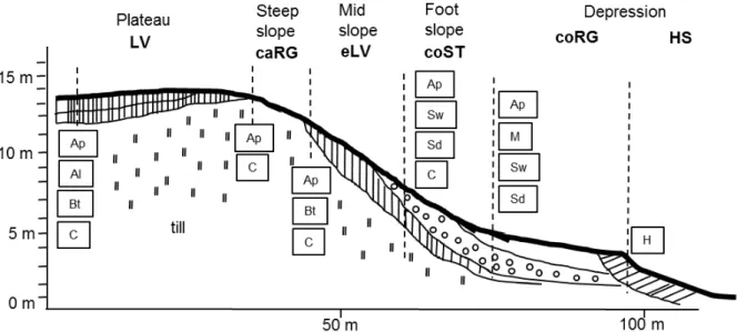
Fig. 1.1. Schematic cross-section through the hummocky moraine landscape of NE Germany with locations of characteristic soil profiles and accompanied soil horizons as well as the typical
geomorphic structures and their soil types. 7
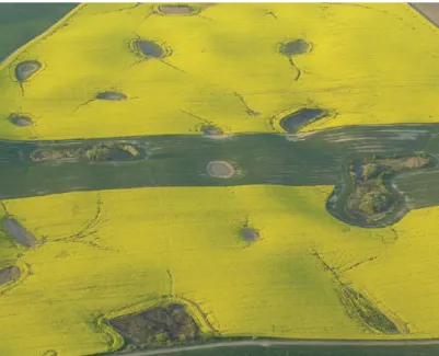
Fig. 1.2. Aerial photograph of the moraine landscape of NE Germany with several kettle holes
distributed in a rapeseed field. 8
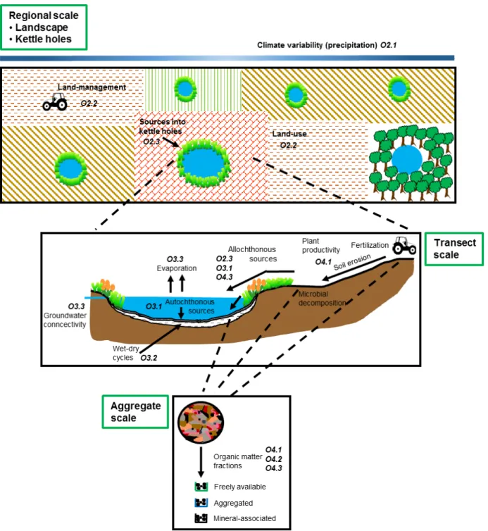
Fig. 1.3. Schematic sketch showing the scales that are target of this study, the mechanisms that may drive C and N dynamics on each scale and the objectives, which shall be answered
on each scale. 22
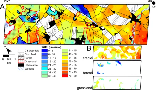
Fig. 2.1. Land-use map from 2013 (A) showing the three dominant land-use types: grasslands, forests and arable fields including the crops cultivated in 2013 and villages. Location of the study site (red rectangle) in the federal state of Brandenburg within Germany (B). 27 Fig. 2.2. Isoscapes of the intrinsic water use efficiency for plants. 32
Fig. 2.3. δ13C soil isoscape. 33
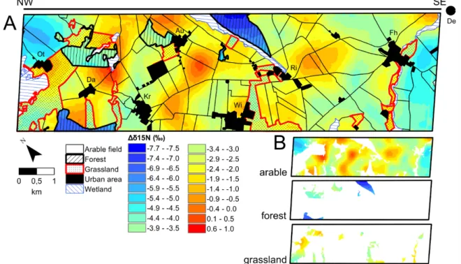
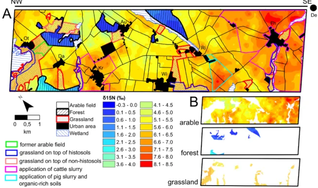
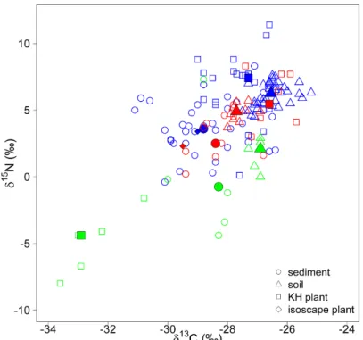
Fig. 2.4. Isoscapes of Δδ15N for plants and soils. 34 Fig. 2.5. Isoscapes of δ15N for soils and land-management effects. 35 Fig. 2.6. Bi-plot of plant, soil, and sediment isotopic composition used in the kettle hole mixing-
model analysis. 37
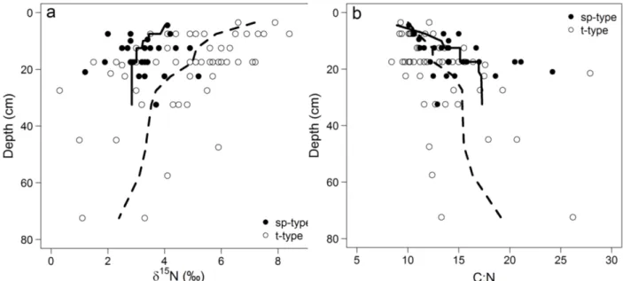
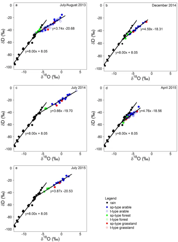
Fig. 3.1. Study site, the location of the study site in NE Germany and photographs of a temporarily water-filled kettle hole in July 2013 the same kettle hole in July 2014. 46 Fig. 3.2. Bi-plot of δ15N vs. the C:N ratio for surface and deeper kettle hole sediments. 51 Fig. 3.3. Bi-plot of the δ15N and the C:N ratio vs. mean depth dimension for each deeper
sediment sample. 52
Fig. 3.4. Bi-plots of δD vs. δ18O of kettle hole water from the different sampling periods. 54 Fig. 3.5. Agglomerative clustering results of kettle hole surface sediment data. 57 Fig. 4.1. Schematic cross-section through the catchment of the kettle hole with assumed differences in biological activity, soil mineral and environmental characteristics between depositional (wetter) and erosional (drier) areas. 69 Fig. 4.2. Elevation map of the catchment with sampling locations. 70 Fig. 4.3. Contents of iron and aluminum extracted by different agents. 78 Fig. 4.4. Proportion of organic carbon contents of organic matter fractions with respect to the total soil organic carbon for each topographic position. 79 Fig. 4.5. Plot of δ13C vs. the natural logarithm of the organic carbon content in the form of a Rayleigh distillation model for each fraction for each topographic position. 81 Fig. 4.6. Plot of δ15N vs. the natural logarithm of the total nitrogen content in the form of a Rayleigh distillation model for each fraction for each topographic position. 82 Fig. 4.7. Conceptual model illustrating the origin and parameters as well as pathways and processes that affect the fate of mineral-associated organic matter fractions. 88
VIII
Fig. 5.1. Summary of the outcomes of the three objectives on the carbon and nitrogen dynamics of different land-use structures and surface sediments from kettle holes from chapter 2 – the
regional landscape scale. 94
Fig. 5.2. Summary of the outcomes of the three objectives on the carbon and nitrogen dynamics in kettle hole sediments of different depth and on the kettle hole hydrology inferred from chapter
3 – the regional kettle hole scale. 96
Fig. 5.3. Summary of the outcomes of the three objectives on the carbon and nitrogen of specific organic matter fractions in the catchment and in subsurface sediments of one semi-permanently water filled kettle hole inferred from chapter 4 – the transect and aggregate scale. 98 Fig. 6.1. Ordinary kriging on the inorganic carbon content of top soils. 104 Fig. 6.2. Ordinary kriging on the soil organic carbon content of top soils. 105 Fig. 6.3. Ordinary kriging on the total nitrogen content of top soils. 106 Fig. 6.4. Methane production in the semi-permanently water-filled kettle holes near the villages
Rittgarten and Kraatz. 110
IX Summary
In moraine landscapes, carbon (C) and nitrogen (N) dynamics can vary greatly across landscape structures and soil types. An integral feature of these landscapes are small inland water bodies, so-called kettle holes, the roles of which on the C and N dynamics of a landscape are often neglected. Given the strong spatial heterogeneity of moraine landscapes, the sole focus on larger (landscape) scale processes may result in the ignorance of small-scale variability in C and N dynamics. To improve predictions of the impacts of global change on landscapes and to ensure their sustainable use, it is essential to identify the driving mechanisms underlying the aquatic-terrestrial C and N dynamics. This study uses stable isotopes to identify these regulating mechanisms across different scales (from regional landscape over kettle hole to aggregate scale) in the moraine landscape of NE Germany – a landscape that is intensively used for agriculture and interspersed with countless kettle holes.
At the regional landscape scale, δ13C isoscapes (isotopic landscapes) of topsoil bulk soil organic matter (SOM) and plant leaves collected from 38.2 km2 landscape unit revealed long- term inputs of organic matter (OM) from C3 crops, which imprinted their water use efficiency status onto the soil, as well as short-term inputs from corn (C4 crop). The δ15N SOM isoscape identified fertilization-induced impacts of land-management on the N dynamics of agricultural fields and grasslands, while showing that the forest N cycle was rather closed.
At the regional kettle hole scale, surface sediments were analyzed for 51 kettle holes located in the same landscape unit but differing with respect to the surrounding land-use type and the hydroperiod. Results for δ13C and δ15N reflected recent OM inputs and processes and pointed at the effect of anoxic sediment conditions and fertilization in the catchment. Deeper sediments recorded the degree to which OM had been processed within the kettle hole depending on the hydroperiod and indicated the burial of OM originating from terrestrial plants.
At the transect scale, erosion and plant productivity were the dominant drivers affecting mineral-associated OM fractions in topsoil sampled along transects spanning erosional to depositional areas in the catchment of one arable kettle hole. In contrast, freely available and aggregated OM fractions were influenced by microbial decomposition and slurry fertilization. At the aggregate scale, the pathway and magnitude of OM-mineral associations changed along the transect while binding OM of different status of decomposition. OM in mineral-associated fractions from sediments was derived from clay- and silt-sized particles from the agricultural field together with emergent macrophyte contributions to freely available and aggregated OM fractions.
By means of stable isotopes techniques, different mechanisms were successfully identified at the individual scales. Consideration of the spatial heterogeneity of all scales from aggregate scale to the entire landscape is essential to understand landscape C and N dynamics.
Small inland water bodies like kettle holes are key constituents with respect to C and N dynamics
X
in moraine agricultural landscapes, because they function as important sinks for OM and alter the environmental conditions in their catchments. However, their net role as C and N sinks or sources in landscapes needs to be determined by future studies comprising longer time scales and more detailed studies on N and C fluxes.
XI Zusammenfassung
Die Kohlenstoff- und Stickstoffdynamiken in Moränenlandschaften können über Landschaftsstrukturen und Bodentypen hinweg stark variieren. Ein besonderes Merkmal dieser Landschaften sind kleine Inlandwasserkörper, die sogenannten Sölle oder Toteislöcher, deren Rolle auf die C- und N-Dynamik der Landschaft oft vernachlässigt wird. Aufgrund der starken räumlichen Heterogenität von Moränenlandschaften kann der alleinige Fokus auf Prozesse auf größeren Skalenebenen (Landschaftsskala) zur Vernachlässigung kleinskaliger Variabilität in der C- und N-Dynamik führen. Um die Voraussagen der Einflüsse des globalen Klimawandels auf Landschaften und deren nachhaltiger Nutzung sicher zu stellen, ist es daher essenziell, die Steuerungsmechanismen der zugrundeliegenden aquatisch-terrestrischen C- und N-Dynamik zu identifizieren. In dieser Studie werden stabile Isotope und deren Verhältnisse genutzt, um diese Mechanismen über verschiedene Skalenebenen (von der regionalen Landschaftsskala bis zur Aggregatskala) hinweg in der Moränenlandschaft von Nordostdeutschland zu identifizieren; einer Landschaft, die stark landwirtschaftlich genutzt wird und in der es eine Vielzahl von Söllen gibt.
Auf der regionalen Landschaftsskala spiegeln δ13C-Isotopenkarten des organischen Materials in Oberböden und von Pflanzenblättern eines 38.2 km2 großen Landschaftsausschnittes zum einen den langfristigen Eintrag von organischem Material von C3- Pflanzen, deren Wassernutzungseffizienz im organischen Material des Bodens eingeprägt wurde, sowie den kurzfristigen Eintrag von Mais (C4-Pflanze) wider. Die δ15N-Isotopenkarte des organischen Materials in Böden weist auf bewirtschaftungsbedingte Einflüsse (v.a.
Düngungseffekte) auf die N-Dynamik von Feldern und Wiesen hin, während der N-Kreislauf in Wäldern eher geschlossen ist.
Auf der im Hinblick auf die Sölle regionalen Skalenebene wurden Oberflächen- sedimente von 51 Söllen mit verschiedener Landnutzung im Einzugsgebiet und unterschiedlicher Wasserführung im o.g. Untersuchungsgebiet analysiert. Die δ13C- und δ15N- Isotopenwerte deuten auf kürzliche Einträge organischen Materials und auf Prozesse wie saisonale Anoxia im Sediment sowie Düngung im Einzugsgebiet hin. Tiefere Sedimente sind hingegen durch die Ablagerung organischen Materials von terrestrischen Pflanzen sowie dessen Umsetzungsgrad geprägt, welcher abhängig von der Wasserführung ist.
Auf der Transekt-Skala, d.h. entlang von Transekten von Erosions- zu Depositionsgebieten im Einzugsgebiet eines Solls in einem Feld, sind Erosion und Pflanzenproduktion die dominanten Steuerungsmechanismen des mineral-assoziierten organischen Materials. Im Gegensatz dazu sind das frei verfügbare und das aggregatgebundene organische Material v.a. durch mikrobielle Umsetzungsprozesse und Gülledüngung beeinflusst. Auf der Aggregat-Skalenebene sind die Art und der Anteil spezifischer organo-mineral Assoziationen entlang des Transekts variabel, wobei organisches
XII
Material verschiedenen Umsetzungsgrades und Ursprungs gebunden ist. In Sedimenten sind Ton- und Siltpartikel vom angrenzenden Feld die dominante Quelle des mineral-assoziierten organischen Materials, während das dort frei verfügbare und aggregatgebundene organische Material terrestrischen Ursprungs ist.
Diese Studie hat erfolgreich stabile Isotopenverhältnisse zur Identifikation von Mechanismen der C- und N-Dynamik auf individuellen Skalenebenen angewendet. Die Berücksichtigung räumlicher Heterogenität auf allen Skalenebenen von der Aggregat- bis zur Landschaftsskala erwies sich als essenziell für das Verständnis der C- und N-Dynamik in der Landschaft. Aufgrund ihrer Funktion als Senken für organisches Material sowie durch die Alteration der Umweltbedingungen im Einzugsgebiet sind kleine Inlandwasserkörper Schlüsselelemente für die C- und N-Dynamik in landwirtschaftlich genutzten Moränenlandschaften. Ihre Rolle als potentielle Netto C- und N-Senken oder -quellen in der Landschaft muss jedoch durch weitere Studien mit längeren Untersuchungszeiträumen und detaillierten Messungen von C- und N-Flüssen gezeigt werden.
1 1. Introduction
1.1 Motivation
Understanding the processes that regulate carbon (C) and nitrogen (N) dynamics in landscapes is crucial in order to make solid predictions on global climate change impacts on the environment and human society (Houghton, 2007; Ussiri and Lal, 2013). Landscapes can be regarded as spatial heterogeneous areas consisting of different landscape structures that encompass both terrestrial and aquatic ecosystems (Premke et al., 2016). Yet, studies attempting to estimate landscape C dynamics often account for terrestrial ecosystems solely, therefore neglecting the role of aquatic inland ecosystems that may considerably increase the C budget of a landscape (Cole et al., 2007). Furthermore, though wetlands and their riparian zones play profound roles in N dynamics of a landscape (Merbach et al., 2002; Verhoeven et al., 2006; Ussiri and Lal, 2013), but are often ignored when trying to assess the N dynamics of a landscape.
Recent estimates suggest that the soil organic carbon (SOC) stock is around
~4000 Pg C and thus higher than the global vegetation and atmosphere C reservoirs combined (IPCC, 2013). As such, even small transformations of SOC into greenhouse gases (GHG) may considerably increase GHG concentrations in the atmosphere (IPCC, 2013). Past estimates suggest that agriculture accounts for ~50 % of global methane (CH4) and for ~60 % of nitrous oxide (N2O) emissions in 2005 (Smith et al., 2007). Agricultural landscapes are therefore under pressure to keep SOC belowground and prevent SOC from transformations into CH4 and CO2, which is in a conflict of interest with their function as ecosystem services. While many studies focus on SOC dynamics in agricultural landscapes solely (e.g. van Oost et al., 2007; Doetterl et al., 2015; Nadeu et al., 2015), microbial transformations of N into N2O and NH3 especially after fertilization practices highlights the importance of N dynamics in agricultural landscapes (Webb et al., 2010; Wolf et al., 2014). Today, agricultural lands occupy 30% to 40% of the earth‘ s ice- free surface (Foley et al., 2005; Smith et al., 2008). Agricultural landscapes show strong interactions between land-use, topography, soil types, microbial activity and climate. To date, large uncertainties especially remain on how land-use and management and climate affect biogeochemical cycles potentially altering the C and N dynamics of the landscape (Doetterl et al., 2016; Premke et al., 2016).
Terrestrial and aquatic C and N dynamics are closely linked to each other because of C, nutrient and mass transfer between both systems. New data show that standing freshwater bodies ≤ 10 ha make up to 10 % (Verpoorter et al., 2014) and ponds < 0.1 ha constitute 8.6 % (Holgerson and Raymond, 2016) of the global inland water surface area. These water bodies are characterized by high perimeter-to-area ratios emphasizing the influences of the littoral zone and allowing for strong aquatic-terrestrial interactions (Palik et al., 2001). Today, there is still a debate about C fluxes in these small ponds and impoundments: on the one hand, they are
2
regarded as C sinks through high OC burial in sediments (Stallard, 1998; Downing et al., 2008) and on the other hand and more recently, they have been identified as hotspots for C cycling in landscapes (Cole et al., 2007; Tranvik et al., 2009; Aufdenkampe et al., 2011; Buffam et al., 2011; Premke et al., 2016).
To successfully estimate terrestrial ecosystem C and N dynamics it is therefore essential to understand the underlying mechanisms of the interactions between the aquatic and terrestrial domains (Premke et al., 2016). In agricultural landscapes in general, beside biological activity (microbial decomposition, plant productivity), and intrinsic soil properties (e.g. texture, moisture, and aggregation), spatio-temporal patterns of SOC largely depend on extrinsic factors like climate, management activities and erosion (Kirkels et al., 2014; Doetterl et al., 2016), with the latter regarded as redistributing large amounts of SOC in moraine agricultural landscapes (Doetterl et al., 2012; Aldana Jague et al., 2016; Sommer et al., 2016).
Moraine landscapes cover around 1.6 × 10¹² m2 of cool-humid climate regions in the northern hemisphere and are often of agricultural use (Sommer et al., 2004). The moraine landscape of NE Germany represents an ideal investigation area since it is widely populated by small (< 1 ha) water bodies, the so-called kettle holes, that are interspersed in the landscape (Kalettka and Rudat, 2006). Hence, they pose the challenge at different spatial scales of organization, which help to characterize the major processes regulating the C and N dynamics across scales: from aggregate to the landscape level. According to Sun et al. (2012) and Zhao and Liu (2014), the sampling density largely determines SOC estimates in agricultural landscapes in general and in the moraine agricultural landscape of NE Germany in particular (Miller et al., 2016). Therefore, investigating C and N dynamics even at small scales and including small water bodies is crucial because the sole focus on the landscape scale may not consider small scale heterogeneities of C and N dynamics and the underlying processes (Kirkels et al., 2014; Hanson et al., 2015; Premke et al., 2016). Moreover, understanding the underlying driving C and N mechanisms at individual scales will allow for better policies to protect and enhance existing SOC stocks and ensure sustainable use of soils (O’Rourke et al., 2015).
1.2 Biogeochemical plant-atmosphere-soil interaction in complex agricultural landscapes Crop productivity is the key element in agricultural landscapes to fulfill their function as food supplier. Climate variability may significantly drive crop production even in fields with high crop yield (Kang et al., 2009). We can expect significant impacts on crop productivity as result of the ongoing global climate, which leads to a rise of carbon dioxide (CO2) in the atmosphere, a temperature increase and more extreme climatic events such as drought (Olesen and Bindi, 2002; Kang et al., 2009). Climatic impacts on plant growth, i.e. via precipitation, may already be investigated at the landscape scale when microclimate variability exists.
3
In addition to nutrient availability and CO2 for photosynthesis, plant productivity heavily relies on water availability. Precipitation is the ultimate source of water in the soil (Vepraskas and Craft, 2016). The vegetation also strongly interfered with the landscape water cycle since plants take up water through their roots during photosynthesis, which is either incorporated (to a very small part) into their biomass or emitted back to the atmosphere through transpiration and thus this water cannot function as groundwater recharge. Provided that sufficient water is available, plants open their stomata and assimilate C while transpiring water (Saurer et al., 1995). However, when the plant is water-stressed, then the photosynthetic activity and therefore plant productivity will be reduced. Changes in the water availability directly leads to changes in the assimilation rate of C, therefore altering the C cycle of the landscape. Assuming now microclimate variability in a given landscape, we can expect differences in the C assimilation rate over the landscape for particular plant species. After plant death, plant biomass enters the soil, where it undergoes and decomposition processes and contributes to the soil organic matter (SOM) pool. Consequently, the C input into soils will be reduced in more dry areas. This directly illustrates the feedbacks between climate, plant productivity and C dynamics in the landscape.
Since agricultural crops have been have developed for specific traits, climate variability may have profound impacts on resisting water deficit of individual plant species (Varshney et al., 2011).
Water availability to plants does not necessarily directly depend on precipitation, but also on the topographic shape of a landscape. The infiltrated water percolates through the pore space following hydraulic gradients. Depending on hydraulic gradients and the soil matrix, the water can remain in the soil where it is either taken up by plants, or directly lost through evaporation, or it can act as groundwater recharge (Vepraskas and Craft, 2016). With respect to the latter, water can collect in wet depressions changing the soil moisture of the adjacent area and providing a water source to plants depending on the topography. Thus, we may expect increasing plant productivity around small wet depressions within an agricultural field.
Next to plant productivity, soil moisture is a key player for the retention of SOM (Sierra et al., 2015). Soil fauna including earthworms, fungi and microbes decompose SOM. While on more elevated landscape positions aerobic microbial decomposition overwhelms, aerobic microbial activity is inhibited in more wet areas due to less oxygen (O2) availability because the pore space is blocked by water (Trumbore, 2009). The combined effects of plant productivity and microbial decomposition taking place at small scales as a result of topography can therefore directly drive the C and N dynamics of the landscape. Another topographic consequence on C dynamics is the transport of soils by erosion, which is a widespread phenomenon in arable landscapes that can alter the distribution and fate of SOM (Lal, 2003; Doetterl et al., 2016). As such, the mechanical stress during the transport of soil particles during water and wind erosion leads to a breakdown of aggregates and makes SOC susceptible to microbes (Lal, 2003). This
4
process may considerably impact the C dynamics of agricultural landscapes. However, there is still a debate ongoing whether soil erosion acts as C sink for atmospheric CO2 (Stallard, 1998;
Berhe et al., 2007; van Oost et al., 2007) or source (Lal, 2008). The criterion whether a watershed acts as CO2 sink is met when the combined effects of dynamic replacement of eroded C by the assimilation of new photosynthate (Harden et al., 1999) and reduced microbial decomposition in the depositional area compensate for C losses through decomposition and leaching at erosional positions (Berhe et al., 2007; Ito, 2007).
Soil erosion in agricultural landscapes is strongly enhanced via land-management practices. Conventional tillage management is common in non-organic farming and enhances the translocation of soil particles, which ultimately reshapes the landscape (Beniston et al., 2015). On smaller scales, tillage favors the breakdown of macro-aggregates and makes the OM more susceptible to microbial decomposition (Paustian et al., 2000; Six et al., 2000). As a second consequence, long-term and strong erosion may remove sorptive minerals and destroy soil matrixes, which may cause water and nutrient losses and in the end reduces plant productivity (Doetterl et al., 2016). With respect to moraine landscapes, tillage erosion can expose the glacial tills with their low clay contents reducing plant growth.
An important practice to improve soil fertility and increase crop yields is the addition nutrients via the application of fertilizers. These may include chemical fertilizers such as urea or ammonium phosphate, or organic manure and compost derived from livestock. The resulting nitrate (NO3-), ammonium (NH4+) and organic N (e.g. amino acids) are taken up by plants and increase plant productivity and plant N level (Choi et al., 2006). After plant death, the N liberated during decomposition contributes to the soil N pool. Since compost may lead to higher soil N levels than the application of chemical fertilizers solely (e.g. Choi et al., 2003), the fertilization pathway may lead to legacy effects on the N levels of a field. Fertilization therefore strongly changes the N cycle, which can be characterized as open N in arable fields. Important N losses are through leaching and gaseous N losses especially after fertilization (Goulding et al., 2000;
Zech et al., 2011). Soil fertility is further improved via catch crops to increase the humus and thus SOC content (Poeplau et al., 2015) as well as to increase soil N content since catch crops retain N from leaching (Constantin et al., 2011). In addition, soil fertility is improved via crop rotations including species differing in their C and N contents. For instance, primary crop species and catch crops can vary in their C:N ratios provided that they are not limited by N (Heal et al., 1997). As such, plant litter with high C:N ratios may cause microorganisms to immobilize N leading to lower decomposition rates, while plant litter with low C:N ratios can be preferentially decomposed since N is no longer the limiting element (Wang et al., 2008; Zhou et al., 2008;
Berhe, 2012). C and N dynamics are additionally altered depending on whether the straw leftovers are removed or remain on the fields (Blanco-Canqui and Lal, 2007; Saffih-Hdadi and
5
Mary, 2008). Consequently, the complex plant cultivation together with fertilization history will considerably alter the C and N dynamics on a field.
Next to arable fields, agricultural landscapes consist of various landscape structures such as forests, grasslands, fallows, hedgerows, villages and water bodies that are present over a range of soil types and topography (Roschewitz et al., 2005). There are not only different landscape structures, but their intrinsic biogeochemical cycles may vary themselves. As such, grasslands can be used for different purpose like pasture, hay and silage production or can be of no use. Furthermore, some grasslands may experience chemical fertilizer or slurry input as an additional N source altering the N cycle of these ecosystems. With respect to forests, deciduous, coniferous or mixed type forests may be different in their C and N dynamics also depending on age and underlying soil types (Bauhus et al., 1998; Côté et al., 2000). Without anthropogenic inputs the N cycle may be regarding closed (Zech et al., 2011). However, forest N dynamics may further be altered by land-management activities performed on adjacent fields.
Land-use changes like the transformation of forests, grassland and wetlands into arable fields to gain more land for food and biofuel production are common all over the world. Several studies showed that starting land-management, the removal of old and the introduction of new plant species considerably change the C and N dynamics of a landscape while often decreasing SOC stocks (Houghton and Goodale, 2004; Poeplau et al., 2011).
Given both the various impacts on the biogeochemical cycles due to land-use changes and management practices as well as the complexity described by different landscape structures, makes it challenging to precisely assess C and N dynamics in agricultural landscapes. We are therefore challenged to develop tools, which may visualize these complex dynamics variable over space and time based on the primary drivers land-use and management and climate.
1.3 The Quillow catchment – a hummocky agricultural landscape in NE Germany
The investigation area from this study is located in the Quillow catchment (~168 km2) as part of the young and hummocky moraine plain of NE Germany that is intensively used for agriculture. The Quillow catchment is part of the Uckermark region, located west of the town Prenzlau and covers parts of the federal states Brandenburg and Mecklenburg-Vorpommern.
The name ‘Quillow catchment’ goes back to the Quillow, which is a stream that drains the Quillow catchment from west to east until it flows into the river Ucker close to Prenzlau.
The settlement and the modulation of land in the Uckermark region started in the 12th century that caused deforestation and led to enhanced agricultural use (Kalettka et al., 2001;
Bayerl, 2006). As such, the proportion of agricultural and pasture use was around 47 % in 1864 (Müller, 1998). In the 18th/19th centuries, agrarian reforms were carried out, which not only led to the separation of fields, but also improved the value of the agricultural soils via dewatering of
6
wetlands (Bayerl, 2006; Kleeberg et al., 2016a). Agricultural intensification due to the
‘Reichsnährstandssgesetz’ during the World War II resulted again in widespread land clearance and the first introduction of fertilizers to improve soil fertility (Neyen, 2014; Kleeberg et al., 2016a). Further agrarian reforms such as the ‘Bodenreform’ and the ‘Flurneuordnung’ carried out the German Democratic Republic (GDR), led in turn to the consolidation and collectivization of agricultural fields with more than 200 ha, industrialization and the absence of erosion- inhibiting structures (Bayerl, 2006; Neyen, 2014; Kleeberg et al., 2016a. Finally, the reunion of the GDR with the Federal Republic of Germany (FRG) introduced new European Union (EU) and German laws that again impacted agricultural use (Kleeberg et al., 2016a).
The hummocky topography of the Uckermark has been shaped during repeated advances and retreats of glaciers during the Weichselian glaciation (Lischeid et al., 2016). The altitude ranges from −1 to 140 a.m.s.l. (Kleeberg et al., 2016a). Owing to the young at of the landscape, the widespread land clearance and agricultural intensification, soils are prone to water and wind erosion (Deumlich et al., 2010). Together with soil redistribution via tillage, the soil landscape is today characterized by a spatial 3D continuum typical for glacial landscapes consisting of mainly sandy to loamy soils (Sommer et al., 2008). However, due to the numerous erosion processes, soils are in a continuous change (Rieckh et al., 2014). In hummocky moraine landscapes, the topsoil is the uppermost due to tillage well-mixed layer referred to as Ap horizon, while the subsoil comprises of the clay-rich Bt horizon underlain by the carbonate-rich glacial till, the C horizon (Fig. 1.1) (Gerke et al., 2010; Deumlich et al., 2010; Gerke and Hierold, 2012). Non-eroded Luvisols (LV) with undisturbed Ap-Al-Bt-C sequences prevail on plateaus, while the relatively sandy Al horizon is a result of the vertical downward transport of clay.
Calcaric Regosols (caRG) prevail on steep slopes, in which the C horizon is already underlying the Ap horizon (FAO classification, IUSS Working Group WRB, 2014). As such, these soils are discernible by the lighter colors in the landscape. Mid slopes are characterized by Eroded, sometimes also Calcic Luvisols (eLV) with the typical Ap-Bt-C sequence. Colluvic Stagnosols (coST) occur on footslopes with Sw and Sd horizons resulted from stagnating water. However, Gleysols (GL) can be found when groundwater affects the soil. Brownish and darker Colluvic Regosols (coRG) with M horizons indicating deposited material are found in depressions. These topographical depressions may have been or are still filled with water during longer periods, in which case Histosols (HS) are the result of the formation of peat bodies. Often, these depressions are referred to as kettle holes.
7
Fig. 1.1. Schematic cross-section through the hummocky moraine landscape of NE Germany with locations of characteristic soil profiles (dashed vertical lines) and accompanied soil horizons (in boxes) as well as the typical geomorphic structures and their soil types (adapted after Gerke and Hierold, 2012). The soil classification is based on the classification the FAO, IUSS Working Group WRB (2014): LV = Luvisol;
caRG = Calcaric Regosol; eLV = Eroded Luvisol; coST = Colluvic Stagnosol; coRG = Colluvic Regosol;
HS = Histosol.
1.4. Kettle holes in the Quillow catchment and their linkage to the terrestrial environment Kettle holes (German: Sölle or Toteislöcher) are widespread features in the Quillow catchment. They can be best described as small pond-like depressional wetlands of glaciofluvial origin. Similar water bodies can be found around the world: in northern America where they are commonly termed ‘pot holes’ (Euliss et al., 2004; van der Kamp and Hayashi, 2009), in other regions of central Europe like Poland (Gołdyn et al., 2015), northern Europe and Asia. Kalettka and Rudat (2006) estimated that 150,000 to 300,000 kettle holes with depressions ranging from 0.01 to 3 ha are present in terminal and ground moraines of NE German that covers approximately 38,000 km2. Since in Germany standing water bodies >1 ha are defined as lakes by nature, the water body of a kettle hole may not exceed 1 ha (Kalettka and Rudat, 2006).
Kettle holes can be primarily found in arable fields with up to 40 per km2 (Fig. 1.2), where they cover approximately 5 % of arable land (Kalettka et al., 2001; Kalettka and Rudat, 2006). They are primarily located in agricultural fields, but also occur in grasslands and forests.
8
Fig. 1.2. Aerial photograph of the moraine landscape of NE Germany with several kettle holes distributed in a rapeseed field (from Premke et al., 2016; picture: G Verch).
Kettle holes were formed due to the delayed melting of buried dead ice blocks after the discontinuous retreat of the Weichselian glaciers approximately 12,000 to 10,000 years ago (Kalettka et al., 2001). ‘True’ kettle holes developed on top of post-glacigenic muds as sealing layers that allowed water to trap in (Kalettka et al., 2001). These kettle holes bear up to 8 m thick fen mires due to organogenic silting up of depressions in natural woodland (Kalettka et al., 2001; Merbach et al., 2002). However, some depressions remained dry due to water deficiency and because they were just relief-caused depressions resulted from the undulated glacial ice (Kalettka et al., 2001; Merbach et al., 2002). The deforestation starting in the 12th century resulted in low water retention in the uplands and increased erosion leading to flooding and continuous silting up of the ‘true’ kettle holes again, which caused a decrease in size of the kettle holes (Kalettka et al., 2001; Merbach et al., 2002). Furthermore, the former dry depressions were flooded and referred to as ‘pseudo’ kettle holes, which lack of post-glacigenic muds, but may comprise of several dm thick peat layers (Kalettka et al., 2001; Merbach et al., 2002). With intensification of agriculture after 1950, kettle holes became obstacles in the agricultural fields and attempts were made to seal or drain them (Kalettka et al., 2001). Today, kettle holes are protected by law because they are biodiversity havens (Pätzig et al., 2012), but protection strategies are not specific enough and are often ignored by farmers (Kalettka and Rudat, 2006). Based on geomorphological and hydrological variables of 268 kettle holes (hydroperiod, shore overflow tendency, depth, area, form, shore width and slope) as well as those of their catchments (area, wetland to catchment area ratio, relief), Kalettka and Rudat (2006) defined 10 hydrogeomorphic types that are regarded to support kettle hole conversation strategies.
9
Due to the young age of the moraine landscape, stream networks could not fully develop yet and therefore most kettle holes are not connected to any streams via groundwater flow (Lischeid and Kalettka, 2012). Kettle holes receive water input primarily in winter and early spring via snowmelt and runoff over partially frozen soils, direct precipitation, and seasonal lateral flow (van der Kamp and Hayashi, 2009; Gerke et al., 2010; Shaw et al., 2012). Water losses are through evapotranspiration, spillover, and lateral shallow groundwater recharge (Berthold et al., 2004; van der Kamp and Hayashi, 2009). Kettle holes can be temporarily in contact with shallow groundwater potentially resulting in discharge or recharge from the groundwater (van der Kamp and Hayashi, 2009; Heagle and others, 2013). Given their location in depressions, kettle holes are especially prone to evaporation as any other stagnant water bodies. To date, no studies exist that describe the connectivity to ground water aquifers nor studies exist that quantify the water losses of kettle holes of NE Germany, though attempts were made to assess water losses of prairie pot holes in northern America (e.g. Ferone and Devito, 2004; Hayashi et al., 1998). Further uncertainties remain on the timing and magnitude of water losses depending on land-use (arable fields, forests, grasslands). Due to climate variability, geomorphic site conditions including site conditions, many kettle hole experience pronounced wet-dry cycles.
The duration of the wet period of a kettle hole over the year is defined as hydroperiod (Kalettka and Rudat, 2006). The resulting pronounced wet-dry cycles can lead to the complete drying and rewetting of some sediments (Johnson et al., 2004; van der Kamp and Hayashi, 2009) while others may stay submerged or partially submerged over the year. Strong water level fluctuations result in changes in OM dynamics and O2 exposure during desiccation (Boon, 2006). The shift in redox conditions, from anoxic to oxic, affect organic matter availability for microbial degradation (Foulquier et al., 2013) and can change microorganism communities or their carbon metabolism, resulting in accelerated OM turnover (Fromin et al., 2010; Reverey et al., 2016; Weise et al., 2016). While in submerged conditions, anoxia is a common phenomenon and causes OM to be less efficiently used for decomposition by heterotrophic microorganisms and could therefore lead to a more intensive burial of OM in the sediment (Sobek et al., 2009).
During long-term wet conditions, internal primary production via phytoplankton and periphytic algae and OM from submerged and floating macrophytes within the kettle hole can be an important autochthonous OM source (lignin-poor OM). On the other hand, desiccation can lead to the encroachment of emergent macrophytes into kettle holes as external OM sources (= allochthonous OM rich in lignin), which may subsequently result in the formation of peat bodies (Gaudig et al., 2006). Thus, the wet-dry cycles impact the environmental site conditions and leave an imprint in the sediment record as distinct layers that may yield information about the sources of OM and the degree of OM microbial decomposition.
10
Kettle holes lie on the boundary between the aquatic and terrestrial domain and are closely linked to their catchments. Due to their location in depression they receive substantial matter input. These include soils via erosion triggered by tillage (Frielinghaus and Vahrson, 1998), plant biomass, nutrients (nitrogen and phosphorous) due to fertilization (Lischeid and Kalettka, 2012) and heavy cation contaminants originating from artificial fertilizers (Gołdyn et al., 2015). Especially the input of nutrients is problematic because it can lead to eutrophication.
Given large shifts in hydroperiod, high eutrophication and resulting high autochthonous OM production and its strong effects on sediment OM transformations, kettle holes might be a potential sources of CO2 and other trace gases (Merbach et al., 2002; Premke et al., 2016).
Furthermore, the general form of land-use, land-management practices have a large influence on terrestrial biogeochemistry. However, broad investigations of kettle hole biogeochemistry in the landscape context are few and we do not know the extent to which external (i.e. terrestrial) factors such as fertilization affect kettle hole internal OM turnover or how this is represented in the sediment column. This is information is crucial do understand kettle holes’ potential as sinks for OM in agricultural landscapes. Due to the water logging of kettle holes, their surroundings can be characterized by steep environmental gradients in moisture and texture (Merbach et al., 2002). Therefore, the moisture gradient may also influence plant productivity and SOM dynamics in the kettle hole catchment.
1.5 Soil organic matter dynamics – small scale processes and their importance on the landscape scale
Dead plant material enters the soil where it undergoes biological, physical and chemical transformations processes that decompose dead plant compounds on different rates depending on their chemical composition. Next to plant-derived molecules, molecules of microbially origin are the second important class in SOM (Schmidt et al., 2011). While microbial decomposition mineralizes a part of OM into inorganic CO2 – therefore termed mineralization – other molecules undergo further transformation and condensation processes into macro-molecules (humification) that where long time regarded as stable against further decomposition (chemical
‘recalcitrant’) and allowed for long-time stabilization of OM in soil (Stevenson, 1994; Lehmann and Kleber, 2015). Nowadays, this traditional view has changed into an emergent view in which SOM can be conceptualized as a continuum of progressively decomposing organic compounds encompassing intact plant material and low molecular, highly oxidized OM such as carboxylic acids (Schmidt et al., 2011; Lehmann and Kleber, 2015). The heterogeneous bulk SOM can be experimentally subdivided into more homogenous fractions of varying mean residence time (MRT) resulting from differences in their stabilization against microbial decomposition. Because of their different turnover dynamics, such fractions have contrasting ecological functions.
11
For example, organic particles with a recognizable morphological structure made up of residues from plants and animals serve as a readily decomposable substrate for soil organisms (Gregorich et al., 2006). Organic particle fractions from surface soils are most sensitive to climatic, land-use or management changes because of their relatively fast turnover and close connection to litter input (Bird et al., 2008). Furthermore, a small part of the soil OM can be present in soil as dissolved OM (DOM) in pore water. OM that is found in the dissolved phase is highly mobile and important when considering vertical (percolation) and lateral (water erosion) transport processes (e.g. Kaiser and Kalbitz, 2012). The DOM is considered in part easily biodegradable (Gregorich et al., 2003; von Lützow et al., 2007) because aqueous mobilization of SOM is postulated to be a critical first step towards its decomposition. However, organic particles as well as DOM in soils are not labile in total but consist of sub-fractions with various degrees of lability (Kalbitz et al., 2003). An explanation might be that organic particles as well as DOM act as binding agents during the formation of aggregates in soils (Golchin et al., 1994;
Six et al., 2000).
The long-term stabilization of OM (MRT > 100 years) in aerated, temperate topsoils against microbial decomposition is highly important for the function of soils to act as a long-term C-sink and to mitigate climate change. Here, microbial access to OM is hindered due to (i) aggregation (Six et al., 2004; Bachmann et al., 2008) (ii) interactions of the OM with polyvalent cations (chelate, crosslinking) (e.g. Masiello et al., 2004; Mouvenchery et al., 2012), (iii) associations of the OM with mineral surfaces via polyvalent cations (cation bridges) (von Lützow et al., 2006), or (iv) direct bond formation between OM and mainly Fe or Al oxides (ligand exchange reactions) (Mikutta et al., 2007; Kleber et al., 2015).
An understanding of the key factors and processes that regulate the OM stabilization in soils requires the separation of stabilized OM fractions according to specific mechanisms (Mikutta et al., 2006). During the last decades, the scientific community has developed numerous physio-chemical. These techniques are physically based only including particle-size separations (Balesdent, 1996), density-separations (Sollins et al., 2009) or combinations of both (Moni et al., 2012). On the other hand, different extraction mediums are used to extract OM such as simply water (Kaiser et al., 2010) or chemical agents (Wagai et al., 2013).
The amount and percentage of OM bound via organo-mineral associations varies greatly between soil types and depth (Kögel-Knabner et al., 2008). Soil erosion leads to the downslope transport of DOM but also of OM that is associated to clay- and silt-sized particles. In addition, organic particles either free or released from disintegrated aggregates (due to tillage or raindrop impact) are preferentially targeted by erosive transport. Especially clay- and silt-sized mineral particles < 53 µm are usually enriched in OC relative to the bulk soil (Hu et al., 2016) as they comprise of comprise of complexed, poorly crystalline and well-crystallized mineral phases as well as clay minerals (e.g. oxides, layer-silicates), which can interact with OM (Kaiser et al.,
12
2007; Doetterl et al., 2015). For instance, erosion may remove reactive minerals phases from erosive areas and accumulate them in depositional areas (Berhe et al., 2012; Ellerbrock et al., 2016). Their preferential transport during erosion events consequently leads to higher SOC concentrations in depositional profiles (Doetterl et al., 2016). As such, understanding OM associated via mineral phases at small scales is crucial to make solid estimates on the SOC distribution in the landscape (O’Rourke et al., 2015).
Where the transport capacity is high enough, the mobilized organic and clay-sized particles might not be deposited but instead may end up in the sediments of water bodies (Stallard, 1998). Yet, large uncertainties remain on the fate of OM in the aquatic ecosystems especially related to changes in climate and land-use (Marín-Spiotta et al., 2014). Stabilization mechanisms of OM in sediments substantiality differ from soils due to the water saturation (Hedges and Oades, 1997). As such, macro-aggregate formation is inhibited, partly because of bioturbation. The amount of OM and stabilization mechanism greatly varies with the oxygen exposure time (Arnarson and Keil, 2007). Organic particles can dominate the OC in sediments with very short oxygen exposure times of < 1 year (anaerobic stabilization), while highly stable mineral-aggregated OM can prevail over oxygen exposure times of several years and even decades (Arnarson and Keil, 2007).During longer exposure times of centuries to millennia, the adsorption of OM to mineral surfaces is the major stabilization mechanism in marine sediments (Mayer, 1994; Hedges and Keil, 1995; Arnarson and Keil, 2007). Recently, Lalonde et al. (2012) found a preferential stabilization of OM via reactive iron surfaces. However, the pathway and as such the amount of OM bound via these iron phases was shown to change from complexation (anaerobic conditions) to poorly and well-crystallized iron phases (Rue and Bruland, 1995;
Lalonde et al., 2012). In general, stabilization mechanisms of sedimentary OM are still largely unknown. Given the water fluctuations of kettle holes with longer wet periods or pronounced wet-dry cycles, the amount and pathway of OM associated in sediments can show large variations over the landscape.
13
1.6 Stable isotopes and their use in environmental sciences
All those described processes may manifest in the stable isotopic composition of OM, which therefore represents an ecological archive. Isotopes are forms of the same element that differ in the number of neutrons in their nucleus (Fry, 2006). The five elements that cycle with OM and that are of particular interest are C, N, O, H and S. Stable isotope ratios are described by the ratio R of the heavy isotope to the light isotope in a sample and referenced to an international standard following EQ. 1.1:
𝛿 = (𝑅𝑅𝑠𝑎𝑚𝑝𝑙𝑒
𝑠𝑡𝑎𝑛𝑑𝑎𝑟𝑑− 1) ∙ 1000 1.1.
Given the usually low differences between the ratio of the sample and the standard, stable isotope ratios are reported in δ notation by multiplying with 1000. In this study, I only focus on C, N, O, and H and as such the ratios are: 13C/12C for δ13C, 15N/14N for δ15N, 18O/16O for δ18O and 2H/1H for δD.
Stable isotopes fractionate during biotic and abiotic processes, i.e. one isotope is preferred against another (Fry, 2006). As such, the difference between the natural isotopic abundance of the educt and the product can be used to gain insights into complex environmental processes (Brüggemann et al., 2011). Two principles of isotopic fractionation occur, which can be related to their system. In a closed system, equilibrium fractionation tries to minimize the energy in a system, i.e. isotopes will be distributed to minimize the vibrational, rotational, and translational energy (White, 2015). This fractionation is primarily temperature- dependent and reversible. Fast, incomplete or unidirectional processes or reactions occur in open systems leading to irreversible kinetic isotopic fractionation (White, 2015). Biologically mediated reactions are typical for causing kinetic isotopic fractionation. As such, plants fractionate against the heavier 13CO2 and take up the lighter 12CO2 during photosynthesis, which is then assimilated into their biomass. This preference of the light isotope will leave the plant leaf depleted in the heavy 13C. The depletion is plant dependent. C3 (3-carbon) plants like trees usually have δ13C values around -28 ‰, while C4 (4-carbon) plants like corn or sugar cane have higher δ13C values around -13 ‰ (Farquhar et al., 1989). This difference in δ13C between C3
and C4 plants is due to differences in primary CO2 fixation (Farquhar et al., 1982). With respect to C3 plants, the C isotopic discrimination during photosynthesis Δ13C can be described by the simplified Farquhar model, which only accounts for the isotopic fractionation during the stomata diffusion a with 4.4 ‰ and the discrimination during carboxylation of RuBisCO b with 27 ‰ following EQ. 1.2 (Farquhar et al., 1982; Farquhar et al., 1989):
∆13𝐶 = 𝑎 + (𝑏 − 𝑎) ∙𝑐𝑐𝑖
𝑎 1.2.
14
Here, ci is the intracellular CO2 content in the stomata and ca represents the ambient atmospheric CO2 concentrations of ~380 ppm. The Δ13C can also be calculated when the δ13C of the atmosphere with -8 ‰ (δ13Ca) and of the plant leaf (δ13Cp) are known (Farquhar and Richards, 1984) following EQ. 1.3:
∆13𝐶 =1+𝛿𝛿13𝐶13𝑎𝐶−𝛿13𝐶𝑝
𝑝/1000 1.3.
The WUEi in µmol C-1 describes the ratio of carbon assimilated A to water transpired E (Farquhar and Richards, 1984). WUEi is generally not directly linked to E, but shows a negative correlation with the ratio of ci/ca. The ratio of ci/ca reflects in turn the balance between A and the stomatal conductance gs after EQ 1.4 (Seibt et al., 2008):
𝐴 = 𝑔𝑠∙ (𝑐𝑎− 𝑐𝑖) 1.4.
Given that gs and the stomatal conductance of the water vapor gsw are related by the constant factor 1.6 (gsw = 1.6 gs), the WUEi calculates according to EQ. 1.5 as follows (Saurer and Siegwolf, 2007; Seibt et al., 2008):
𝑊𝑈𝐸𝑖 = 1.6𝑐𝑎 ∙𝑏−𝛿13𝑏−𝑎𝐶𝑎+𝛿13𝐶𝑝 1.5.
Consequently, there the WUEi can be directly calculated based on the δ13C of the plant leaf. Provided that sufficient water is available, plants open their stomata to take up 12CO2
resulting in a high ci, while assimilating less carbon in their biomass (low A) and transpiring water (high gs). This will result in lower δ13C values. However, during drier conditions, plants close their stomata to avoid water loss (low gs), whereas no new 12CO2 can be taken up (low ci), but carbon will be assimilated (high A), leading in the end to higher δ13C values. As such, the δ13C of plant can be used as a proxy of the water availibility to a plant over time in the landscape.
In contrast to C, N sources to plants a more complex. N sources encompass NH4+, NO3-
, dissolved organic nitrogen (DON; e.g. amino acids) and atmospheric N2 in N limited systems (Houlton et al., 2007). The enzymatic formation of these N sources in the soil system is often accompanied by the discrimination against the heavy isotope 15N (Robinson, 2001). As such, nitrification causes an enrichment in 15N in the remaining NH4+ in aerobic soils, while denitrification leads to higher contents of 15N in the remaining NO3- in more anaerobic soils (Mariotti et al., 1981; Robinson, 2001; Choi et al., 2003). However, the isotopic discrimination is much larger for nitrification causing higher δ15N values of the remaining NH4+ (Mariotti et al., 1981; Casciotti et al., 2003). It is generally accepted plants can discriminate against 15N directly or indirectly via mycorrhizal fungi leading to lower δ15N values in plant leaves compared to the N source (Robinson, 2001; Houlton et al., 2007; Hobbie and Högberg, 2012). However, changes in NH4+:NO3- uptake ratios, the use of atmospheric N2 with a δ15N of ~ 0 ‰, or the use of high
15
DON high in δ15N can further change the foliar δ15N (Evans, 2001; Houlton et al., 2007; Kahmen et al., 2008; Takebayashi et al., 2010). When the plants leaves remain in the system are returned to the N-soil pool by plant litter degradation, and no additional losses N inputs/occur, then the N cycle can be characterized as closed (Zech et al., 2011). In this case, with an ultimate only atmospheric N2 source, the soil δ15N could be expected to be close to 0 ‰.
However, the N cycle in agricultural landscapes can usually not characterized as closed given N losses via the harvest of plants and land-management practices as N sources. Organic manure is known to be enriched in 15N due to the preferential loss of 14N during ammonia (NH3) volatilization (Kreitler, 1979; Kerley and Jarvis, 1996) and was found to range from +5 - 20 ‰ (Heaton, 1986; Yoneyama et al., 1990; Choi et al., 2003; Bateman et al., 2005). Volatilization continues after application on the field leading to high N emissions (Webb et al., 2010). Nutrients (NH4+, NO3-) originating from the manure will be enriched in 15N (Choi et al., 2003). The uptake of these enriched nutrients can lead to higher δ15N values in plants (Bateman et al., 2005; Choi et al., 2006; Senbayram et al., 2008). On the other hand, it is known that chemical fertilizers such as urea or ammonium phosphate are less enriched in 15N as they originate from atmospheric N2 (Choi et al., 2003; Michalski et al., 2015). Consequently, δ15N of plants were found to be lower when only chemical fertilizers were applied (e.g. Choi et al., 2006). After plant death, the plant OM with its high δ15N contributes to the bulk SOM leaving the soil enriched in
15N (Yoneyama et al., 1990; Choi et al., 2003). As such, high δ15N values of soils are indicative for an open N cycle. One way to get stronger insights into the N cycle is the calculation of the Δδ15N as the difference between δ15Nplant and δ15Nsoil (Amundson et al., 2003; Kahmen et al., 2008). While on global scales temperature and precipitation are of importance on the Δδ15N (Amundson et al., 2003), differences in the NH4+/NO3- uptake ratios dominate at local scales (Kahmen et al., 2008; Takebayashi et al., 2010). Therefore, the δ15N of SOM can be a complex archive of multiple processes and sources in the landscape.
An important C and N loss in soils is given by microbial decomposition, which can be also described as kinetic isotopic fraction. During aerobic decomposition, microbes preferentially take of the light isotopes 12C and 14C leaving the residual OM enriched in the heavy isotopes 13C and 15N (Torn et al., 2002; Dijkstra et al., 2008; Craine et al., 2015). This process leads to a downward increase in δ13C and δ15N in soil profiles (Meusburger et al., 2013). The enrichment is especially assumed in mineral-associated OM fractions and increases with density (Sollins et al., 2009; Schrumpf et al., 2013), decreases with particle size (Asano and Wagai, 2014) and is also found in chemically extracted fractions (Kayler et al., 2011). Since other studies found lower δ13C with decreasing particle size (Hu et al., 2016), microbial decomposition can be variable. Furthermore, microbial decomposition is accompanied by a decrease in the C:N ratio of the residual OM because of the catabolic loss of C (Paul and Clark, 1996). However, anaerobic microbial decomposition may either lead to no enrichment or even