LECTURE ”HIGHER MATHEMATICS” PART I Vector Calculus

(1)

LECTURE ”HIGHER MATHEMATICS”

PART I

Vector Calculus

(2)

1 Spatial vectors

A vectorain physical space is an arrow, pointing from some point P to another pointQ.

Themagnitude (length) |a| ≥0 ofais defined as the linear distance between P and Q.

Generally, a vector a is fixed by its magnitude and its direction. As an arrow is shifted in space, without changing magnitude and direction, it still describes the same vector.

1.1 Vector algebra

Asa points from P toQ and b from Q toR,vector addition is defined by

c = a + b, (1)

wherec is the vector pointing from P toR.

Multiplication ofa with a real numberλ ∈Rshall, by definition, yield another vector

a⁰ = λa (2)

with length|a⁰|=|λ||a| and direction parallel (λ >0) ore opposite (λ <0) to a.

Forλ=−1, we also write

λa ≡ (−1)a = −a, a + (−1)b = a −b. (3)

We choose three mutually orthogonal directions ”1”, ”2”, and ”3” (which shall form a right-handed system). Then, a typical vector is written as

a =



 2 m

−5 m 4 m



 =



 a₁ a₂ a₃



 = a₁



 1 0 0





| {z }

=a₁

+ a₂



 0 1 0





| {z }

=a₂

+ a₃



 0 0 1





| {z }

=a₃

, (4)

wherea₁ is the vector with length a₁ = 2 m pointing in direction 1, a₂ is the vector with length −a₂ = 5 m pointing opposite to direction 2, a3 is the vector with length a3 = 4 m pointing in direction 3.

The dimensionless objects u₁ =



 1 0 0



, u₂ =



 0 1 0



, u₂ =



 0 0 1



, (5) with |u_n|= 1, are called unit vectors,

a = a₁u₁ + a₂u₂ + a₃u₃. (6) The numbers a_n are called the coordinatesof the vector a. Theorem of Pythagoras:

|a| = q

a²₁+a²₂+a²₃. (7)

The vectors a_n are called the components of the vector a.

(3)

Vectors may have units other than length. While the an are carrying the physical units of the vectorial quantitya, the u_n are ”dimensionless”. E.g., a force vectoris

F = F₁u₁ + F₂u₂ + F₃u₃

= (2.13 N)u1 + (−1.95 N)u2 + (4.79 N)u3

= (2.13 N)



 1 0 0



+ (−1.95 N)



 0 1 0



+ (4.79 N)



 0 0 1



 =





2.13 N

−1.95 N 4.79 N



. (8) Itsmagnitude is |F| = p

F₁²+F₂² +F₃² ≈ 5.59 N.

1.2 Scalar (dot) and vector (cross) products

The scalar product (or dot product) of two vectors aand b is defined as

a·b := |a||b|cosγ (a number !), (9) whereγ is the angle between aand b.

Consequently, b·a=a·b and, with some λ∈R, (λa)·b=λ(a·b).

Furthermore, (a+b)·c=a·c+b·c (see problem 1.1), and thus a·b ≡ (a₁u₁+a₂u₂+a₃u₃)·(b₁u₁+b₂u₂+b₃u₃)

≡ X³

i=1

a_iu_i

·X³

j=1

b_ju_j

=

3

X

i=1 3

X

j=1

a_ib_j(u_i·u_j)

| {z } δ_ij

=

3

X

i=1

a_ib_i ≡ a₁b₁ +a₂b₂+a₃b₃. (10)

Therefore, in terms of the coordinates, a·b ≡



 a₁ a₂ a3



·



 b₁ b₂ b3



 = a₁b₁+a₂b₂+a₃b₃. (11)

Let u⊥ be the unit vector perpendicular to both a and b, such that {a,b,u⊥} is right-handed. Thevector product (or cross product) of a with b is defined as

a×b :=

|a||b|sinγ

u⊥ (a vector !). (12)

Sinceb×a=−a×b and (λa)×b =λ(a×b), etc. (exercises), we now have a×b ≡ ... = a₂b₃−a₃b₂

u₁ + a₃b₁−a₁b₃

u₂ + a₁b₂−a₂b₁

u₃. (13) Therefore, in terms of the coordinates,



 a₁ a₂ a₃



×



 b₁ b₂ b₃



 =





a₂b₃−a₃b₂ a₃b₁−a₁b₃ a₁b₂−a₂b₁



. (14)

(4)

2 Curves in space: Vector functions of one argument

2.1 Orbit of a moving particle as an example

Selecting one pointO in space as origin, any other pointP is fixed by itsposition vector r = OP~ = xu1+yu2+zu3. (15) The position vector of a moving particle has time-dependet coordinates x, y, and z,

r(t) =



 x(t) y(t) z(t)



. (16)

This is a vector function. As t grows, the tip of the vector r(t) “draws” the orbit of the particle which is a curve in space.

Example 1a: Motion on a helical (helix shaped) orbit is described by the function

r(t) =





Rcos(ωt) Rsin(ωt)

ut



. (17)

2.2 Derivative of vector functions: velocity vector

The derivative of a vector function r(t) is another vector function ˙r(t), defined as

˙

r(t) ≡ d

dtr(t) := lim

∆t→0

r(t+∆t)−r(t)

∆t (18)

≡ lim

∆t→0

1

∆t





x(t+∆t)−x(t) y(t+∆t)−y(t) z(t+∆t)−z(t)



 ≡





˙ x(t)

˙ y(t)

˙ z(t)



. (19) The vectorsr(t) andr(t+∆t) (blue) and their difference (green) are shown in Fig. 1.

Figure 1: .

(5)

At any given timet, the magnitude of the vector ˙r(t) is

|r(t)|˙ = lim

∆t→0

r(t+∆t)−r(t)

∆t

= lim

∆t→0

|r(t+∆t)−r(t)|

∆t . (20)

For sufficiently small∆t(when orbital curvature becomes negligible), the numerator|r(t+

∆t)−r(t)|approaches the distance∆son the orbit, travelled by the particle between times t and t+∆t. Consequently, the limit (20) is the temporaryspeed v(t) of the particle,

|˙r(t)| ≡ p

˙

x(t)²+ ˙y(t)²+ ˙z(t)² = ∆s

∆t = v(t). (21)

As is obvious from the figure, the direction of the vector ˙r(t), indicated in red color, is tangentialto the orbit at r(t). Therefore, the vector

v(t) ≡ r(t)˙ (22)

is called thevelocity (vector) of the particle.

Example 1b: In Example 1a, we obtain

˙ r(t) =





−Rωsin(ωt) +Rωcos(ωt)

u



, v(t) = p

(Rω)²+u² ≡ v. (23)

2.3 Parametrization of a curve

Instead of t, any monotonic functionp(t) may serve as a parameter p of a curve, r(p) =



 x(p) y(p) z(p)



. (24)

A typicalexample is the arc length p(t) = s(t) along the curve, s(t) =

Z t 0

dt⁰ r(t˙ ⁰)

≡ Z t

0

dt⁰p

˙

x(t⁰)²+ ˙y(t⁰)²+ ˙z(t⁰)². (25)

Example 1c: For the curve of Example 1a, we obtain s(t) =

Z t 0

dt⁰p

(Rω)²+u² ≡ vt ⇒ r(s) =





Rcos(^ω_vs) Rsin(^ω_vs)

u vs



. (26)

Exercise: Writing ^dr(p)_dp = ˙r(p), we findchain and product rules for vector functions d

dtr p(t)) = r(p)˙

p=p(t)p(t),˙ (27)

d dp

h

r₁(p)·r₂(p)i

= r˙₁(p)·r₂(p) + r₁(p)·r˙₂(p). (28)

(6)

2.4 Unit tangent vector

Since the vector ˙r(p) is tangential to the orbit, the (”normalized”) vector TTTTT(p) = r(p)˙

|˙r(p)| =



 T₁(p) T₂(p) T3(p)



 (29)

is theunit tangent vector of the orbit.

As a consequence,TTTTT(p)· TTTTT(p) = 1 and the product rule yields

0 = d

dp

hTTTTT(p)· TTTTT(p)i

= 2 TTTTT(p)· dTTTTT(p)

dp ⇒ dTTTTT(p)

dp ⊥ TTTTT(p). (30) Consequently, the vectors TTTTT(p) and ^dT^T^T^T^T_dp^(p) are orthogonal to each other.

Remark 1: When p=s is the arc length along the curve (with |˙r(s)|= 1), we write dTTTTT(s)

ds =: 1

ρ(s)NNNN(s)







|NNNN(s)|= 1, ρ(s)≥0.

(31)

• NNNN(s), the unit normal vector, points toward the center of that circle in space which best approximates the curve at the point r(s).

•ρ(s) is the radius of that circle (”radius of curvature”).

Remark 2: Choosing again the time t as parameter, with v(t) = ^ds(t)_dt ≡s(t), we have˙ v(t) ≡ r(t) =˙ v(t)TTTTT s(t)). (32) Taking here the derivative _dt^d (for the second time), we obtain another vector function of time t which is called the vectora(t) of the particle’s acceleration,

a(t) ≡ ¨r(t) = v(t)˙ TTTTT s(t)) + v(t) d

dtTTTTT s(t)

= v(t)˙ TTTTT s(t)) + v(t) d dsTTTTT(s)

s=s(t)

˙ s(t)

|{z}

v(t)

= ¨s(t)TTTTT s(t)) + s(t)˙ ²

ρ s(t)NNNN s(t)

. (33)

We see that a(t) has a component ¨s(t)TTTTT s(t)) tangential to the orbit of the moving particle, but, in addition, also has a component _ρ(s(t))^s(t)^˙ ² NNNN s(t)

normal to the orbit.

Consequently, while |v(t)|=|s(t)|, we have˙

|a(t)| = v u u

ts(t)¨ ² +

"

˙ s(t)² ρ s(t)

#2

≥ |¨s(t)|. (34)

(7)

3 Scalar fields

A scalar field is a function f that assigns a number

f(r) ≡ f(x, y, z) (35)

to each pointr = (x, y, z) in space.

Examples: T(x, y, z) can be the air temperature (in K) in a room or the temperature distribution in a solid,ρ(x, y, z) the density (in mg/m³) of CO₂ in air (e.g., above a city).

[In addition, these values are typically changing with timet,T =T(x, y, z, t), etc.]

3.1 Graphical representations

3.1.1 2D fields: 3D plot

An example for a 2D scalar field f(x, y) is the temperature T(x, y) on a planar metal surface (xy-plane). As a model, we consider the simple analytical function

T(x, y) = y

1 +x². (36)

Such a function with only two variables can be illustrated by a graph in 3D space: For each point (x, y) on the xy-plane consider the numberz =T(x, y) as the third coordinate of apoint (x, y, z) in 3D space above (or, for z <0, below) the xy-plane.

x 0 1 2 3 0 1 2 3

y 1 1 1 1 2 2 2 2

z 1.0 0.5 0.2 0.1 2.0 1.0 0.4 0.2

For a few selected points (x, y) in the xy-plane (black dots), the resulting points (x, y, z) are plotted in Fig. 2 (red dots). The union of all these image points forms a curved surface in 3D space, indicated by blue curves in Fig. 2, called the3D plot of f.

Figure 2: 3D plot of the function T(x, y) = _1+x^y 2 (blue solid curves).

(8)

3.1.2 2D fields: Contour plot

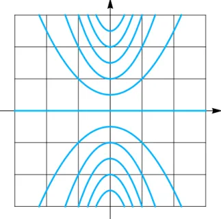
Alternatively, we can plot curves of constant temperature in the xy-plane: Resolving T(x, y) ≡ y

1 +x² = z (37)

fory (we could resolve for x as well), we find

y = z(1 +x²)

≡ y_z(x). (38)

For each fixed value of z, this equation describes a curve in the xy-plane, joining points with constant temperatureT(x, y) =z. For z ∈ {0.5,1.0,1.5, ...}, these ”isothermals” on the xy-plane are shown as blue curves in Fig. 3.

Figure 3: Contour plot of the functionT(x, y) = _1+x^y 2 (blue solid curves).

Such a set of curves in thexy-plane is called acontour plotof the scalar fieldT(x, y).

Figure 4: Contour plot of the functionT(x, y) = _1+x^y 2 in thexy-plane (blue solid curves).

(9)

3.2 Partial derivatives

For a given scalar fieldf(x, y, z), the three functions (scalar fields as well!) fx(x, y, z) ≡ ∂

∂xf(x, y, z) := lim

h→0

f(x+h, y, z)−f(x, y, z)

h ,

f_y(x, y, z) ≡ ∂

∂y f(x, y, z), fz(x, y, z) ≡ ∂

∂z f(x, y, z) (39)

are called itspartial derivatives. They are evaluated in the same way as the derivative of a function with onlyonevariable, treating all the other variables simply as parameters.

Example: The partial derivatives of f(x, y, z) =x²ycos(z²) are

∂f

∂x = 2xycos(z²), ∂f

∂y =x²cos(z²), ∂f

∂x =−2x²yzsin(z²). (40) For a 2D scalar fieldf(x, y), the partial derivatives are visible in the 3D plot of Fig. 2:

•f_x(x₀, y₀) is the slope of the tangent (green) to the curve z=f(x, y₀) in thexz-plane,

•f_y(x₀, y₀) is the slope of the tangent (green) to the curve z =f(x₀, y) in the yz-plane, both tangents drawn at the point (x₀, y₀, z₀), where z₀ =f(x₀, y₀).

3.3 Gradient

To find an alternative way of illustrating, applicable also to a 3D fieldf(x, y, z), we take the quantities ^∂f_∂x and ^∂f_∂y as the coordinates of a column vector

Gf(x, y) = _∂

∂xf(x, y)

∂

∂yf(x, y)

≡

fx(x, y) f_y(x, y)

. (41)

This vector G_f(x, y), actually a vector field, is called the gradient of the scalar field f at the pointr= (x, y). Introducing the nabla operator∇,

∇ = _∂

∂x∂

∂y

, (42)

the gradient is usually written as

Gf(x, y) = ∇f(x, y) ⇔ Gf(r) = ∇f(r). (43)

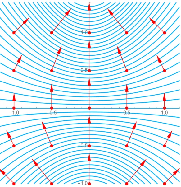
At the point (x₀, y₀) on the planar metal surface (xy plane), the vector G_T(x₀, y₀) = ∇T(x, y)

x=x0,y=y0

(44) points into that direction where the temperature is increasing at the strongest rate.

Consequently, it is exactly perpendicular to the corresponding curve in the contour plot.

(10)

-1.0 -0.5 0.5 1.0

Figure 5: Gradient field of the function T(x, y) = _1+x^y 2 (red arrows).

A 3D scalar fieldf(x, y, z) such as the air temperatureT(x, y, z), cannot be represented graphically (since there is no such thing as a “4D plot”!). In this case, the gradient is a 3D column vector,

G_f(x, y, z) := ∇f(x, y, z) ≡





fx(x, y, z) f_y(x, y, z) f_z(x, y, z)



, ∇ :=





∂

∂x∂

∂y∂

∂z



. (45) Still, now in 3D space, this vector points into the direction where the function f(x, y, z), e.g., the air temperatureT(x, y, z), increases at the strongest rate.

(11)

3.4 Multiple integrals

3.4.1 Double or surface integrals

On a water surface (xy-plane), letρ(x, y) be the mass density (in µg/cm²) of an oil film, representing a 2D scalar field. For simplicity, we assume the function

ρ(x, y) =





 ρ₀

1 − x² +y² R²

(x²+y² ≤R²) 0 (x²+y² ≥R²)







, ρ₀ = 2.7 µg

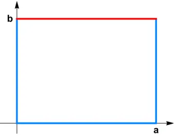
cm², R = 0.50 m.(46) From the functionρ(x, y), we wish to compute the amount m_Ω of oil (in µg) distributed within a given piece Ω of water surface, e.g., the right triangle (red in Fig. 6)

Ω = n

(x, y)∈R²

0≤x≤a, 0≤y≤ bx a

o

(a, b >0, a²+b² < R²). (47)

For an approximate solution to this problem, we introduce small step sizes ∆x and

∆y, generating a mesh of discrete points r_ij in the xy-plane (black dots in Fig. 6), r_ij = (x_i, y_j) = (i·∆x, j·∆y) (i, j ∈Z). (48)

Figure 6: The right triangle Ω (red) and the position vectors r₄₁ and r₃₄ (blue).

For sufficiently small∆x and∆y, the amount∆mij of oil within the small rectangle with side lengths∆xand ∆y, centered at the point r_ij, is approximately given by

∆m_ij ≈ ∆x·∆y·ρ(x_i, y_j). (49) Considering all pointsr_ij ∈Ω (green in Fig. 6) and taking the sum, we have

m_Ω ≈ X

rij∈Ω

∆m_ij =

imax

X

i=imin

∆x





jmax(i)

X

j=jmin(i)

∆y·ρ(x_i, y_j)



. (50) For the situation in Fig. 6, e.g., the outer sum has the fixed limitsi_min = 0 and i_max = 4, while the limitsj_min and j_max of the inner sum are depending on the current value of i:

j_min(i) = 0 (∀i), j_max(0) =j_max(1) = 0, j_max(2) = 1, j_max(3) = 2, j_max(4) = 3.

(12)

At this point, it is easy to see¹ that the limit ∆x,∆y →0 yields the double integral m_Ω =

Z xmax

x_min

dx

Z ymax(x) y_min(x)

dy ρ(x, y), (58)

wherex_min andx_max are the extreme values of the x-coordinates of all points (x, y) in Ω, whiley_min(x) andy_max(x) are, for a given value of x, the ones of the y-coordinates,

m_Ω = Z a

0

dx Z bx/a

0

dy ρ(x, y). (59)

1Fixed by the boundary of the domain Ω ∈ R², the numbers imin and imax depend on ∆x and, for eachi, the numbersjmin(i) andjmax(i) depend on∆y, with the limits

lim

∆x→0

i_min·∆x

= x_min, lim

∆x→0

i_max·∆x

= x_max; (51)

∆y→0lim

j_min(i)·∆y

= y_min(x_i), lim

∆y→0

j_max(i)·∆y

= y_max(x_i), (52) where xmin/xmax are the smallest/largest x-coordinates of any r ∈ Ω, while ymin(x)/ymax(x) are the smallest/largesty-coordinates of anyr∈Ω with givenx-coordinatex.

E.g., for the triangleΩ in Fig. 6/Eq. (47), we have

xmin= 0, xmax=a, ymin(x)≡0, ymax(x) = bx

a. (53)

The approximation (50) becomes exact in the limit∆x,∆y→0,

m_Ω = lim

∆x→0 i_max

X

i=i_min

∆x



 lim

∆y→0 j_max(i)

X

j=jmin(i)

∆y ρ(x_i, y_j)



. (54) Obviously, for any fixed value of xi, the limit [...] in squared brackets is the ordinary integral of the functionf(y)≡ρ(xi, y),

lim

∆y→0 jmax(i)

X

j=j_min(i)

∆y f(y_j) =

Z ymax(xi) y_min(x_i)

dy f(y). (55)

It can be evaluated in the familiar way, Z y_max(x_i)

y_min(x_i)

dy ρ(xi, y) = ρ0

Z bx_i/a 0

dy(A−By²)

A= 1− x²_i

R², B = 1 R²

= ρ0

Ay−B

3 y³

y=bxi/a y=0

= ρ0

b

axi − b aR²

1 + b²

3a²

x³_i

≡ F(xi). (56) In a second step, the limit∆x→0 in Eq. (54) yields the ordinary integral ofF(x),

m_Ω = lim

∆x→0 imax

X

i=i_min

∆x F(x_i)

=

Z xmax

xmin

dx F(x)

= Z a

0

dx F(x) = ρ₀ ab

2 − ab

12R²(3a²+b²)

= ρ₀ab 2

1−3a²+b² 6R²

. (57)

These two subsequent integrations are usually written as the double integral of Eq. (59).

(13)

In evaluating a double integral, we first perform the “inner“ (here: y) integration (note that the upper limitbx/a of they integral depends on the variable xof the ”outer”

integral!), treating the other variablex as a constant parameter, m_Ω =

Z a 0

dx Z bx/a

0

dy ρ₀

1 − x²+y² R²

= Z a

0

dx Z bx/a

0

dy ρ0

R²

R² − (x²+y²)

= ρ₀ R²

Z a 0

dx Z bx/a

0

dy R² −x² −y²

= ρ₀ R²

Z a 0

dx

R²−x²

y − y³ 3

y=bx/a y=0

= ρ₀ R²

Z a 0

dx bR²

a x − b

a + b³ 3a³

x³

. (60)

Remaining is an ordinary integral over onevariable x, m_Ω = ρ₀

R² bR²

a x²

2 − b

a + b³ 3a³

x⁴ 4

a 0

= ρ₀ab 2

1− 3a²+b² 6R²

. (61)

Remark: It is also possible, to take the y integral as the outer one. Then, however, the integration limits must be re-defined,

m_Ω = ρ₀ R²

Z ymax

ymin

dy

Z xmax(y) xmin(y)

dx R²−y²−x²

= ρ₀ R²

Z b 0

dy Z a

ay/b

dx R²−y²−x²

= ρ₀ R²

Z b 0

dy

R²−y²

x − x³ 3

x=a x=ay/b

= ρ₀ R²

Z b 0

dyh

R²−y² a−a

by

− 1 3

a³ − a³ b³y³i

= ρ₀ R²

Z b 0

dyh

aR² − a³ 3

− aR²

b y − ay² + a b + a³

3b³

y³i

(62) Again, we are left with an ordinary integral overonevariable y,

m_Ω = ρ₀ R²

h

aR² − a³ 3

b − abR²

2 − ab³

3 + ab³

4 + a³b 12

i

= ρ₀hab

2 − ab

12R²(3a²+b²)i

. (63)

The result, of course, cannot depend on the particular way chosen for evaluating the integrals. It is completely fixed by the domainΩ ⊆R² and by the integrand (scalar field) ρ(x, y)≡ρ(r). Therefore, we use the notation

m_Ω = Z

Ω

d²r ρ(r), (64)

and call this thedouble integral of the scalar field ρ(r) over the domain Ω ⊆R².

(14)

Example: We consider the circle Ω with radius a and center at r=0, Ω = n

(x, y)∈R²

x²+y² ≤a²o

. (65)

In this case, x_min, x_max =∓a and y_min(x), y_max(x) = ∓√

a²−x², Z

Ω

d²r ρ(r) = ρ₀ R²

Z a

−a

dx Z

√ a²−x²

−√ a²−x²

dy R²−x²−y²

= ρ₀ R²

Z a

−a

dx

(R²−x²)y− y³ 3

y=√ a²−x²

y=−√ a²−x²

= ρ₀ R²

Z a

−a

dx

(R²−x²)2√

a²−x²− 2

3(a²−x²)^3/2

= ρ₀ R²

Z a

−a

dx

2

R²−a² 3

− 4 3x²

√

a²−x². (66)

From standard integral tables (e.g.: Bronstein, integrals nos. 157 and 159), we extract Z

dx√

a²−x² = 1 2

x√

a²−x² + a²arcsinx a

, (67)

Z

dx x²√

a²−x² = a² 8

x√

a²−x² + a²arcsinx a

− x

4(a²−x²)^3/2, (68) to find

Z

Ω

d²r ρ(r) = ρ0

πa² − πa⁴ 2R²

. (69)

This derivation is simplified considerably by using polar coordinates, see Eq. (94) below.

3.4.2 Triple or volume integrals

Integrals of scalar fieldsf(r) over a 3D domain Ω are called tripleorvolume integrals, Z

Ω

d³r f(r) =

Z xmax

xmin

dx

Z ymax(x) ymin(x)

dy

Z zmax(x,y) zmin(x,y)

dz f(x, y, z). (70) Again, the order of these three integrations may be chosen differently, when the limits of each integral are re-defined properly.

Example: Let Ω be a pyramid with height H and quadratic base with side a, Ω = n

(x, y, z)

0≤z ≤H, 0≤ |x|,|y| ≤ a 2

1− z

H o

. (71)

In this case, we choose the z integral as the outer one to obtain Z

Ω

d³r f(r) =

Z zmax

zmin

dz

Z xmax(z) xmin(z)

dx

Z ymax(z) ymin(z)

dy f(x, y, z)

= Z H

0

dz

Z ^a₂(1−^z

H)

−^a₂(1−_H^z)

dx

Z ^a₂(1−^z

H)

−^a₂(1−_H^z)

dy f(x, y, z). (72) For the simple function f(x, y, z) =az, this integral will be evaluated in Eq. (78) below.

(15)

3.4.3 Average value of a function

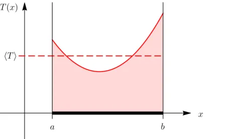
A solid rod, lying on the x-axis (with its endpoints at x= a and at x =b), may have a non-uniform (x-dependent) temperature distribution, given by a function T(x).

T(x)

hTi

a b

x

Figure 7: The rod on the x-axis (black), its non-uniform temperature distribution (red curve), and its average temperature (dashed red line).

From the figure, it is obvious that the average temperatureof the rod is given by hTi = 1

L Z b

a

dx T(x), (73)

whereL=b−a is the length of the rod.

Instead of the rod, covering the 1D interval Ω = [a, b]⊂R with length LΩ =b−a, we may also consider a thin metal sheet, covering a 2D surfaceΩ ⊂R² with area A_Ω, or a piece of solid material, covering a 3D region Ω ⊂R³ with volume V_Ω.

Area A_Ω and length L_Ω can each be called a ”volume” V_Ω in D-dimensional space (withD= 2 and D= 1, respectively). In this spirit, we generally define:

Def.: The average value of a scalar field T(r) in aD-dimensional domain Ω ⊂R^D is D

T(r)E

r∈Ω ≡ 1

V_Ω Z

Ω

d^Dr T(r), (74)

whereV_Ω is the D-dimensional ”volume” of Ω (with D= 3, D= 2 or D= 1).

Example 1: Consider a metal sheet covering the ”upper half ” Ω of a disk, Ω = n

(x|y)∈R²

x²+y² ≤a², y ≥0o

(V_Ω ≡A_Ω = π

2a²). (75) Given the functionT(x, y) =T₀· ^y_a, the average temperature on the sheet is

D T(r)E

r∈Ω = 1

π 2a²

Z a

−a

dx Z

√ a²−x²

0

dy T₀· y a

= 2

πa² T₀

a Z a

−a

dx y²

2

√ a²−x²

0

= 4

3πT₀. (76)

(16)

Example 2: Inside the pyramid Ω of Eq. (71) the temperature shall increase linearly from 0^◦C at the floor (z = 0) to some maximum value T₀ at the tip (z =H),

T(r) = T₀

H z ≡ T(x, y, z). (77)

Given the volumeV_Ω = ¹₃a²H of this pyramid, the average temperature inside is D

T(r)E

r∈Ω ≡ 1

V_Ω Z

Ω

d³r T(r)

= 3

a²H Z H

0

dz

Z ^a₂(1−_H^z)

−^a₂(1−_H^z)

dx

Z ^a₂(1−_H^z)

−^a₂(1−_H^z)

dyT₀ H z

= 3T₀ a²H²

Z H 0

dz

Z ^a₂(1−^z

H)

−^a₂(1−_H^z)

dxh

zyiy=^a₂(1−_H^z) y=−^a

2(1−^z

H)

= 3T₀ a²H²

Z H 0

dz

Z ^a₂(1−_H^z)

−^a₂(1−_H^z)

dx za 1− z

H

= 3T₀ a²H²

Z H 0

dz h

za

1− z H

x

ix=^a₂(1−^z

H) x=−^a

2(1−^z

H)

= 3T₀ a²H²

Z H 0

dz za² 1− z

H 2

= 3T₀ H²

Z H 0

dz z³

H² − 2z² H +z

= T₀

4 . (78)

Remark A: Computing a volume (in 3D or in 2D).

For the trivial functionT(r)≡1, we have hT(r)iΩ = 1, implying the formula V_Ω =

Z

Ω

d^Dr1. (79)

Example 3: Find the volume V_Ω of the tetrahedron Ω, bounded by the four planes x= 0, y= 0, z = 0 and ^x_a +^y_b +^z_c = 1 (with a, b, c >0; SKETCH!),

VΩ = Z

Ω

d³r1 = Z a

0

dx

Z b(1−^x

a) 0

dy

Z c(1−^x

a−^y

b) 0

dz1

= c Z a

0

dx

Z b(1−^x

a) 0

dy 1−x

a − y b

= c Z a

0

dxh 1− x

a

y−y² 2b

i^y=b(1−^x_a) y=0

= bc Z a

0

dxh 1−x

a 2

− 1 2

1−x a

2i

= bc 2

Z a 0

dx 1−x

a 2

= −bc 2

Z 0 1

adu u² = abc

6 . (80)

(17)

Remark B: Double integral as a 3D volume

LetΣ be a domain in thexy-plane, fixed by xmin,xmax, ymin(x), and ymax(x).

Then, the double integral of a 2D scalar field f(r) = f(x, y) is Z

Σ

d²r f(r) =

Z xmax

xmin

dx

Z ymax(x) ymin(x)

dy f(x, y)

≡

Z xmax

xmin

dx

Z ymax(x) ymin(x)

dy

Z f(x,y) 0

dz1, (81)

where we have utilized the trivial identityf(x, y) =Rf(x,y)

0 dz1.

Consequently, provided that f(r) ≥ 0 for r ∈ Σ, the double integral R

Σd²r f(r) equals the volume of the 3D region Ω bounded by Σ and the (curved) 3D-plot off,

Z

Σ

d²r f(r) = Z

Ω

d³r1. (82)

Example 4: The tetrahedral volume from example 2 can also be obtained as the double integral of the 2D scalarfield f(x, y) = c(1− ^x_a− ^y_b)≡z over Σ ={(x, y)∈R²|...},

V_Ω = Z

Σ

d²r f(r) = c Z a

0

dx

Z b(1−x/a) 0

dy 1− x

a −y b

= ... = abc

6 . (83)

(18)

4 Curvilinear coordinates

4.1 Planar polar coordinates

The position vectorr of a point P in the xy-plane with cartesian coordinates (x, y), r = xu₁+yu₂ =

x y

, (84)

is fixed as well by its planar polar coordinates(r, φ):

r =|r| 0≤r <+∞ Lengthof r Distance of P from the origin O.

φ 0≤φ <2π Azimuth angle of r Angle from the x-axis to r (ccw)

x y

φ

r

4.1.1 Coordinate lines

We express the “old” coordinates (x, y) in terms of the “new” ones (r, φ), r(r, φ)≡

x(r, φ) y(r, φ)

=

rcosφ rsinφ

. (85)

This is a vector function oftwo variables (r and φ).

• For fixed φ = φ₀ and r growing from r = 0 to r = ∞, the point r(r, φ₀) in the xy-plane moves on a ray to infinity, starting at the origin.

• For fixed r =r₀ and φ growing from φ= 0 to φ= 2π, the point r(r₀, φ) moves ccw on a circle of radius r₀ centered at the origin.

These rays and circles are thecoordinate lines of planar polar coordinates.

(19)

4.1.2 Double integrals

As in section 3.4.1, letρ(x, y) be the 2D mass density of a thin oil film on a water surface (xy-plane R²). To compute the amount m_Ω of oil distributed within a given piece Ω of water surface (red pentagon in the figures below), we introduce a grid of coordinate lines.

x y

Ω

x y

Ω

Cartesiancoordinate lines (left part of the figure) cut thexy-plane into small rectangles (”tiles”) with side lengths ∆x, ∆y, and with the uniform surface area (per tile)

∆A = ∆x·∆y. (86)

By proper choice of the coordinate lines, these cartesian tiles have their midpoints at r_ij =

x_i yj

, (87)

where x_i = i·∆x and y_j = j ·∆y (with i, j ∈ Z). Consequently, the amount m_ij of oil distributed within the tile atr_ij is approximately given byρ(r_ij)·∆A,

m_ij ≈ ρ(r_ij)·∆x·∆y, (88)

which becomes exact in the limit ∆x,∆y→0.

Polarcoordinate lines (right part of the figure) cut the xy-plane into curved tiles which, spanning a small angle∆φ, are sections of concentric rings with thickness ∆r. For small

∆φ, such a curved tile, with outer and inner radiir±¹₂∆r, is approximately rectangular, with side lengths∆r and r∆φ. Consequently, the surface area per tile is r-dependent,

∆A(r)e ≈ r·∆r·∆φ. (89)

In terms ofx(r, φ) and y(r, φ) from Eq. (85), these tiles have their midpoints at sαβ =

x(rα, φβ) y(r_α, φ_β)

, (90)

where r_α = α·∆r and φ_β = β·∆φ (with α, β = 1,2,3, ...). Consequently, the amount me_αβ of oil distributed within the tile at s_αβ is approximately given byρ(s_αβ)·∆A(re _α),

me_αβ ≈ ρ(s_αβ)r_α·∆r·∆φ, (91)

which becomes exact in the limit ∆r,∆φ→0.

(20)

Eq. (88) for cartesiancoordinates implies [cf. Eq. (50) in section 3.4.1]

m_Ω ≈ X

rij∈Ω

m_ij ≈

imax

X

i=imin

∆x

jmax(i)

X

j=jmin(i)

∆y·ρ(x_i, y_j)

→

Z xmax

xmin

dx

Z ymax(x) ymin(x)

dy ρ(x, y). (92)

Similarly, writingρ(s_αβ)≡ρ x(r_α, φ_β), y(r_α, φ_β)

= ˜ρ(r_α, φ_β), Eq. (91) yields

m_Ω ≈ X

s_αβ∈Ω

me_αβ =

αmax

X

α=αmin

∆r

βmax(α)

X

β=βmin(α)

∆φ·r_α·ρ(r˜ _α, φ_β)

→

Z rmax

rmin

dr

Z φmax(r) φmin(r)

dφ rρ(r, φ).˜ (93)

The extra factorJ(r, φ) =rin the integrand is theJacobianof planarpolarcoordinates.

Example 1: For the disk Ω with radius a of Eq. (65), Eq. (66) now becomes m_Ω =

Z

Ω

d²r ρ(r) = Z a

−a

dx Z

√a²−x²

−√ a²−x²

dy ρ(x, y), ρ(x, y) = ρ0

R² h

R²−(x²+y²)i

= Z a

0

dr Z 2π

0

dφ rρ(r, φ)˜

= ρ₀ R²

Z a 0

dr Z 2π

0

dφ r(R²−r²)

= ρ₀ R²

Z a 0

drh

(R²r−r³)φiφ=2π φ=0

= ρ₀ R²

Z a 0

dr2π(R²r−r³)

= ρ₀ R²2π

R² r²

2 − r⁴ 4

r=a r=0

= ρ₀

πa² − πa⁴ 2R²

. (94)

Example 2: If Ω, more generally, is a section of a circular ring, we have Z

Ω

d²r f(r) = Z r2

r1

dr Z φ2

φ1

dφ rf(r, φ).˜ (95)

Remark: For general curvilinear coordinates (v, w), the surface area ∆Ae of the curved tile depends on both v and w. The correspondingJacobian J(v, w) is defined by

J(v, w) = lim

∆v,∆w→0

∆A(v, w)e

∆v·∆w. (96)

For small butfinite ∆v and ∆w, we then have ∆A(v, w)e ≈ J(v, w)·∆v·∆w and m_Ω =

Z vmax

vmin

dv

Z wmax(v) wmin(v)

dw J(v, w) ˜ρ(r, φ). (97) Generally, the Jacobian is the determinant of thefunctional matrix,

J(v, w) = det

∂x(v, w)/∂v ∂x(v, w)/∂w

∂y(v, w)/∂v ∂y(v, w)/∂w

. (98)

(21)

4.1.3 Scale factors

Consider the partial derivatives of the two-argument vector functionr(r, φ), h_r(r, φ) = ∂r(r, φ)

∂r = ∂

∂r

rcosφ rsinφ

=

cosφ sinφ

, h_φ(r, φ) = ∂r(r, φ)

∂φ = ∂

∂φ

rcosφ rsinφ

=

−rsinφ +rcosφ

. (99)

At each pointr(r, φ), these are tangential vectorsto the two coordinate lines.

The magnitudes

4.2 Spherical (polar) coordinates

The position vectorr of a point P in xyz-space with cartesian coordinates (x, y, z), r = xu1+yu2+zu3 =



 x y z



, (102)

is fixed as well by its spherical (polar) coordinates (r, θ, φ):

r 0≤r <∞ Length|r|of r Distance of P from the origin O.

θ 0≤θ≤π Polar angleof r Angle between r and thez-axis (polar axis) u₃ φ 0≤φ <2π Azimuth angle of r Angle in the xy-plane from thex-axis u₁ (ccw)

to the projection r_xy of r onto thexy-plane

4.2.1 Coordinate lines and surfaces

We express the “old” coordinates (x, y, z) in terms of the “new” ones (r, θ, φ), r(r, θ, φ)≡





x(r, θ, φ) y(r, θ, φ) z(r, θ, φ)



=





rsinθcosφ rsinθsinφ

rcosθ



. (103)

This is a vector function ofthree arguments (r,θ, and φ).

(22)

Keeping two arguments fixed, we are generating the coordinate lines:

• The point r(r, θ₀, φ₀), with growing r, moves on a ray, starting at r=0.

• The point r(r₀, θ, φ₀), with growing θ, moves on a vertical semi circle.

• The point r(r₀, θ₀, φ), with growingφ, moves on a horizontalcircle.

Keeping onlyone argument fixed, we are generating the coordinate surfaces:

• The point r(r₀, θ, φ) moves on a spherical surface with radius r₀.

• The point r(r, θ₀, φ) moves on a conical surface with opening angleθ₀.

• The point r(r, θ, φ₀) moves on a semi plane, bounded by the z-axis.

Except for points on the z-axis, the functions x(r, θ, φ),y(...),z(...) can beinverted:

•Generally (including points on the z-axis), we have r(x, y, z) = p

x²+y²+z². (104)

•For r6=0 ⇔ r6= 0, we have

θ(x, y, z) = arccosz r

≡ arccos z

px²+y²+z², (105)

while θ is not defined for r= 0.

•Eventually, for x²+y² 6= 0, we have

φ(x, y) =











arctan^y_x (x >0, y ≥0), π/2 (x= 0, y >0), π+ arctan^y_x (x <0),

3π/2 (x= 0, y <0), 2π+ arctan^y_x (x >0, y <0),

(106)

while φ is not defined for points on the z-axis (withx²+y² = 0).

4.2.2 Triple integrals

A sphere (radius R, center at the origin) has the electric dipole charge density

ρ(r) ≡ ρ(x, y, z) = a·z (a >0). (107) (What is the physical dimension of the constanta >0 ?)

The amount qΩ of charge on the upper half sphere Ω (z ≥0), Ω = n

(x, y, z)

x²+y²+z² ≤R², z≥0o

, (108)

(23)

is in cartesian coordinates given by the triple integral Z

Ω

d³r ρ(r) = Z R

−R

dx Z

√R²−x²

−√ R²−x²

dy Z

√

R²−x²−y²

0

dz ρ(x, y, z). (109) In terms ofspherical polar coordinates (r, θ, φ), writing

˜

ρ(r, θ, φ) = ρ rsinθcosφ, rsinθsinφ, rcosθ

, (110)

the limits of this integral are simplified considerably, Z

Ω

d³r ρ(r) = Z R

0

dr Z π/2

0

dθ Z 2π

0

dφ J(r, θ, φ) ˜ρ(r, θ, φ), (111) with the Jacobian of spherical polar coordinates,

J(r, θ, φ) = r²sinθ. (112)

This extra factor arises, since

∆V₀ = ∆r·∆θ·∆φ·J(r₀, θ₀, φ₀) = ∆r·(r₀∆θ)·(r₀sinθ₀∆φ) (113) is the volume of the small almost-cuboid

∆Ω =







r(r, θ, φ)

r₀− ¹₂∆r ≤ r ≤ r₀+ ¹₂∆r, θ₀ −¹₂∆θ ≤ θ ≤ θ₀+ ¹₂∆θ, φ₀− ¹₂∆φ ≤ φ ≤ φ₀+¹₂∆φ







(114) surrounding the pointr₀ =r(r₀, θ₀, φ₀).

Now, using ˜ρ(r, θ, φ) =a·rcosθ, we can evaluate the integral, Z

Ω

d³r ρ(r) = Z R

0

dr Z π/2

0

dθ Z 2π

0

dφ r²sinθ (a·rcosθ)

= 2πa Z R

0

dr Z π/2

0

dθ r³sinθ cosθ

= 2πa Z R

0

dr r³

2 sin²θ π/2

0

= πa r⁴

4 R

0

= π

4aR⁴. (115)

(24)

4.2.3 Scale factors

Consider the partial derivatives of the three-argument vector functionr(r, θ, φ), h_r(r, θ, φ) = ∂r(r, θ, φ)

∂r = ∂

∂r





rcosθ



 =





sinθcosφ sinθsinφ

cosθ



,

h_θ(r, θ, φ) = ∂r(r, θ, φ)

∂θ = ∂

∂θ





rcosθ



 =





rcosθcosφ rcosθsinφ

−rsinθ



,

h_φ(r, θ, φ) = ∂r(r, θ, φ)

∂φ = ∂

∂φ





rcosθ



 =





−rsinθsinφ rsinθcosφ

0



,

(116) At each pointr(r, φ), these are tangential vectorsto the three coordinate lines.

The magnitudesh_u(r, θ, φ)≡ |h_u(r, θ, φ)|

h_r(r, θ, φ) = 1, h_θ(r, θ, φ) = r, h_φ(r, θ, φ) = rsinθ, (117) are called scale factors. Again, their product yields the Jacobian,

J(r, θ, φ) = |h_r| |h_θ| |h_φ| = r²sinθ. (118)

4.3 General (orthogonal) curvilinear coordinates

Generalizing (r, θ, φ), we now consider any set α = (u, v, w) of three coordinates which uniquely specify the cartesian coordinates (x, y, z) of each point r in space

r(u, v, w) ≡





x(u, v, w) y(u, v, w) z(u, v, w)



 = r(α), (119)

with somefunctions x(u, v, w),y(u, v, w), and z(u, v, w).

4.3.1 Scale factors

Tangential vectors to the three coo.-lines throughr(α) are given by h₁(α) = ∂r(α)

∂u , h₂(α) = ∂r(α)

∂v , h₃(α) = ∂r(α)

∂w . (120)