Climate change impact on Sub-Saharan Africa

(1)

(2)

(3)

Climate change impact on Sub-Saharan Africa

An overview and analysis of scenarios and models

Christoph Müller

Bonn 2009

(4)

Müller, Christoph: Climate change impact on Sub-Saharan Africa : an overview and analysis of scenarios and models / Christoph Müller. – Bonn : DIE, 2009 – (Discussion Paper / Deutsches Institut für Ent- wicklungspolitik ; 3/2009)

ISBN 978-3-88985-451-3

Dr. Christoph Müller works as scientist at the Potsdam Institute for Climate Impact Research (PIK). His research focuses on global land-use patterns, climate impacts on agricultural production, global biogeo- chemical cycles, and climate-vegetation feedbacks.

℡ +49 (0)228 94927-0 +49 (0)228 94927-130 E-Mail: die@die-gdi.de www.die-gdi.de

(5)

Abbreviations

Summary 1 1 Introduction 5

2 Climate projections 5

2.1 Common emission scenarios 6

2.2 Climate models 8

2.3 Regional climate change projections for Africa 15

2.3.1 GCM performance for Africa 15

2.3.2 GCM projections for Africa 19

2.3.3 Downscaling of GCM climate projections 25

2.4 Conclusions on the suitability of climate projections for impact assessments 26 3 Impact projections 28

3.1 Agriculture 29

3.2 Water availability 33

3.3 General natural trends and biodiversity 35

4 Conclusions 37

4.1 Gaps and uncertainties in models and scenarios 37

4.2 Dealing with uncertainty in climate change impact studies 38 4.3 Relevance for politics of uncertainty in climate change impacts 40

Bibliography 43

(6)

Figure 1: Relative contributions to uncertainty in the simulation of climate

change over Europe originating from various sources 6 Figure 2: Schematic overview of the 4 Special Report on Emission Scenarios

(SRES) scenario families (A1, A2, B1, and B2) 7

Figure 3: Multivariable Taylor diagrams of the 20th century CMIP3 annual cycle

climatology (1980–1999) 14

Figure 4: Global climate network temperature stations 16 Figure 5: Temperature anomalies with respect to 1901 to 1950 for Africa and

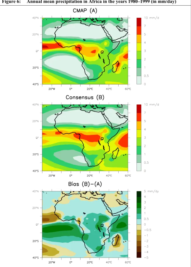
three sub-Sahara African land regions for 1906 to 2005 20 Figure 6: Annual mean precipitation in Africa in the years 1980–1999 (in mm/day) 23 Figure 7: The annual mean temperature response in Africa in 21 CMIP3 models 24 Figure 8: Temperature and precipitation changes over Africa from the CMIP3-A1B

simulations 25 Figure 9: The annual mean precipitation response in Africa in 21 CMIP3 models 27

Figure 10: Projected impacts of climate change, ordered by global mean annual

temperature change relative to 1980–1999 28

Figure 11: Climate change impacts on cereal production under the A2 scenario

by 2080 32

Figure 12: Water stress in the 2050s for the A2 scenario based on withdrawals to

availability ratio 34

Figure 13: Changing water stress between “current conditions” and the 2050s

for the A2 scenario 35

Figure 14: Number of people (millions) with an increase in water stress (Arnell 2006) 36 Tables

Table 1: Overview of SRES scenario characteristics 8

Table 2: Selected model features of the AOGCMs 10

Table 3: Biases in present-day (1980–1999) surface air temperature and

precipitation in the CMIP3 simulations 18

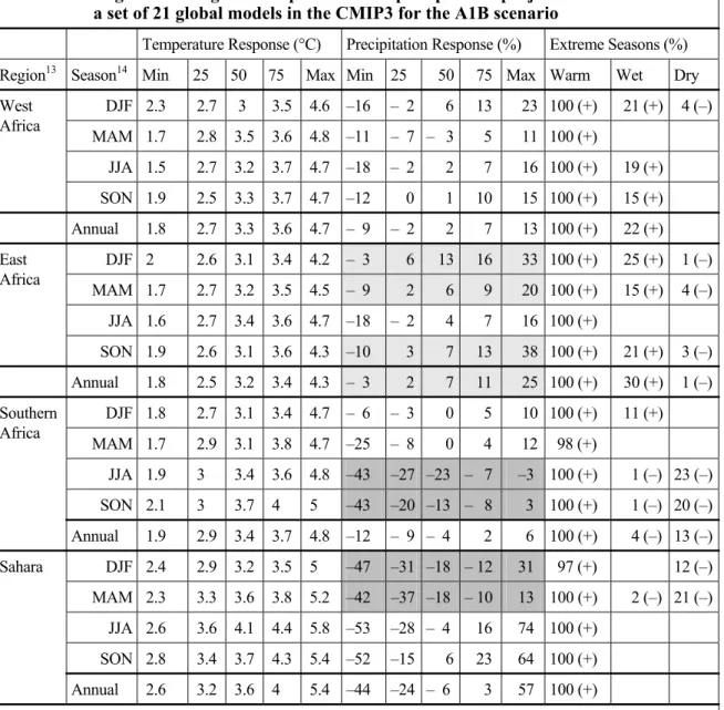
Table 4: Regional averages of temperature and precipitation projections for

Africa from a set of 21 global models in the CMIP3 for the A1B scenario 21 Table 5: Significant ecosystem responses estimated in relation to climate change

in Africa 37

Note: A coloured version (Figures and Tables) of this Discussion Paper is available online at http://www.die-gdi.de (publications).

(7)

A1 A SRES scenario (see Table 1) A1B A SRES sub-scenario (see Table 1) A1C A SRES sub-scenario (see Table 1) A1F1 A SRES sub-scenario (see Table 1) A1G A SRES sub-scenario (see Table 1) A1T A SRES sub-scenario (see Table 1) A2 A SRES scenario (see Table 1)

AGCM Atmosphere General Circulation Model AOGCM Atmosphere-Ocean General Circulation Model B1 A SRES scenario (see Table 1)

B2 A SRES scenario (see Table 1) BCC-CM1 A climate model (see Table 2) BCCR-BCM2.0 A climate model (see Table 2) CCSM3 A climate model (see Table 2) CGCM3.1 A climate model (see Table 2) CMAP A precipitation data set

CMIP3 Coupled Model Intercomparison Project Phase 3 CNRM-CM3 A climate model (see Table 2)

CSIRO-MK3.0 A climate model (see Table 2)

CO2 Carbon dioxide

C3 A carbon fixation mechanism in photosynthesis C4 A carbon fixation mechanism in photosynthesis

DJF December, January, February

DSSAT Decision Support System for Agrotechnology Transfer

EAF East Africa

ECHAM5/MPI-OM A climate model (seeTable 2) ECHO-G A climate model (see Table 2)

EMIC Earth System Model of Intermediate Complexity

ENSO El-Niño Southern Oscillation

EPIC Erosion Productivity Impact Calculator FACE Free Air Carbon Enrichment

FGOALS-g1.0 A climate model (see Table 2) GAEZ Global Agro-Ecological Zones

GCM General Circulation Model

GDP Gross Domestic Product

GFDL-CM2.0 A climate model (see Table 2) GFDL-CM2.1 A climate model (see Table 2)

GHG Greenhouse Gas

GISS-AOM A climate model (see Table 2) GISS-EH A climate model (see Table 2) GISS-ER A climate model (see Table 2)

hPa Hectopascal (10² Pa)

IETC International Environmental Technology Centre INM-CM3.0 A climate model (see Table 2)

(8)

IPCC Intergovernmental Panel on Climate Change IPSL-CM4 A climate model (see Table 2)

JJA June, July, August

km Kilometer(s)

MAM March, April, May

MIROC3.2 A climate model (see Table 2) MRI-CGCM2.3.2 A climate model (see Table 2) MtC Million tonnes of Carbon equivalent

NAO North Atlantic Oscillation

PCM A climate model (see Table 2)

PCMDI Program for Climate Model Diagnosis and Intercomparison

RCM Regional Climate Model

SAF Southern Africa

SON September, October, November

SRES Special Report on Emission Scenarios

SST Sea Surface Temperature

UKMO-HadCM3 A climate model (see Table 2) UKMO-HadGEM1 A climate model (see Table 2)

UNEP United Nations Environment Programme

WAF West Africa

WCRP World Climate Research Programme

WRI World Resources Institute

(9)

Summary

Significant climate change is expected over the 21st century; it will affect ecosystems and access to natural resources such as fertile land and water. Regions with low adaptive capacity due to poverty, lack of infrastructure, services, and appropriate governance will be most severely affected. Sub-Saharan Africa is, due to its low economic development and the diversity of local conditions, a region that needs special attention in developing adaptation strategies.

Climate impacts and the adaptive capacity of societies determine their vulnerability to climate change. The extent of climate change and spatial patterns of impacts are, however, highly uncertain. This report supplies background knowledge on climate change in sub- Saharan Africa, including uncertainties and basic assumptions of climate change projections. Impact studies are only roughly summarized here, as a systematic evaluation of the wealth of specific case studies available would by far exceed the scope of this report.

Climate will change in the future, driven by human emissions of greenhouse gases (GHGs), among which carbon dioxide (CO2) is the most important and most prominent.

Assessing future climate change is very uncertain for the following reasons:

— Future changes in drivers of climate change are uncertain, a circumstance usually addressed by employing different scenarios on GHG emissions (see Section 2.1);

— due to their high complexity, climate models can offer no more than reduced representations of the climate system, which is also not fully understood in terms of all mechanisms (see Section 2.2); and

— several feedbacks exist between climate change and its drivers, e. g. the impact on agricultural production, which affects land requirements for agricultural production, and these in turn drive land-use and land-cover change, a driver of climate change.

Most climate models are able to reproduce observed African climate in its general patterns (i. e. overall trends, large-scale spatial patterns), but they often display strong deviations on the more detailed level: average temperatures are too cool in most reference simulations (reproduction of observed historic climate), and annual and seasonal precipitation simulations sometimes deviate strongly from observations (see Table 3). Also, simulated rainfall intensities typically indicate too many days with light precipitation and too few heavy precipitation events. Research on more specific aspects of African climate, such as climate extremes, is limited and often highly uncertain. E. g. projections on changes in monsoon patterns and cyclones are too uncertain to allow for general conclusions. Despite these deviations and some systematic errors in reproducing observed climate patterns, climate models reproduce the observed climate trend at the continental and regional scale reasonably well. Climate projections can therefore be employed to assess the range of possible future climate change, keeping in mind the shortcomings of climate projections for Africa, and in general.

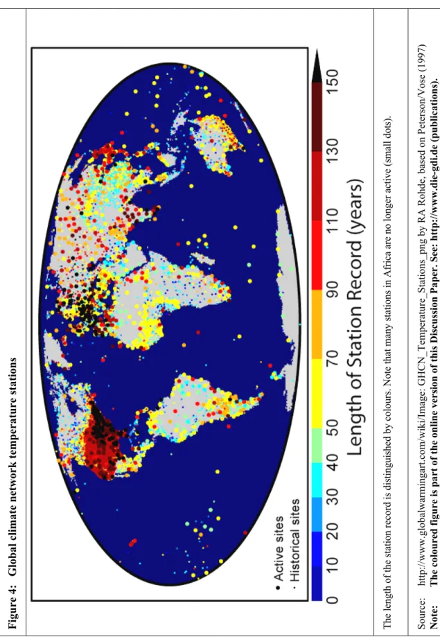
Downscaling projections of coarse climate models for assessments of regional and local climate change impacts adds to the overall uncertainty in climate change projections. This is especially true for Africa, where the climate observation network is not as dense as in other continents (see e. g. Figure 4), because downscaling methods require high-resolution reference data. Besides, downscaled regional climate data are less easily accessible and often only selected scenarios and time slices are available.

(10)

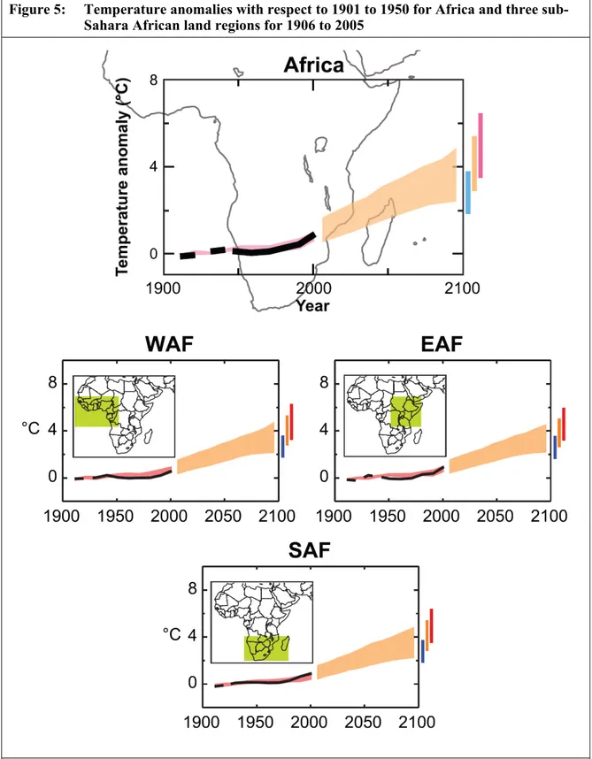
Climate change projections for Africa agree that Africa will experience a strong warming trend over the 21st century (roughly +2.0 to +4.5° C by 2100 in sub-Saharan Africa), which is expected to be stronger than the global average. Most climate models agree on the spatial pattern of temperature change in Africa (with the strongest warming in the Sahara region and southern Africa), although the magnitudes of temperature change projections differ considerably (see e. g. Figure 7). Projections of changes in precipitation patterns are less uniform among climate models. Even when considering only one driving emission scenario, there is, for almost every region in Africa, at least one climate model that projects an increase in precipitation and at least one that projects a decrease (see e. g. Figure 9). No focal area for climate change impact analyses can be identified from available climate change projections: all regions are expected to warm over the 21st century, and almost all will in all likelihood experience declining precipitation (see e. g. Table 4).

Climate projections and the underlying emission scenarios are highly uncertain, while general impact assessments are still largely lacking. Impacts of climate change have not been systematically evaluated yet and overviews of climate change impacts are typically based on a collection of case studies. These case studies typically differ in terms of basic assumptions as well as of cultural, social, and environmental conditions and are thus hard to compare or generalize. Large-scale studies on the other hand may fail to provide sufficient accuracy at the local level. For assessments of vulnerability and political advice, these gaps need to be bridged with general assumptions. Quantitative impact studies are not broadly available – and when they are, they only consider a small selection of scenarios, use general assumptions on climate change or stylized climate scenarios (see Section 3).

There is little consistency between different studies on time frame and coverage of climate projection uncertainty. Often studies address either short-term changes (up to 2020/2030), mid-term changes (2040–2050), and/or long-term changes (2080–2100), but there usually is no justification for the time frame selected.

Climate change impacts on agriculture at larger scales are usually assessed with statistical or econometric means deduced from changes in vegetation period or with the GAEZ model, a simplified crop model driven by a comprehensive database on climate, soil properties, and management. Smaller-scale assessments usually address very specific conditions and employ more detailed crop growth models such as DSSAT, EPIC, or many other field-scale crop models. There have been several attempts to apply detailed crop growth models at the global scale, but these are still in their infancy and no future projections are available yet.

Assessments of water stress often only consider surface water availability per capita, ne- glecting water quality, water demand, direct utilization of rainfall for plant growth, and the possibility of technical adaptation measures. Especially in African agriculture, measures of soil water conservation and rain water harvest yield some potential to mitigate water shortages.

In spite of all the uncertainties in climate change and impact projections, there is a broad consensus that Africa in particular will experience severe climate change. Even though the local specifics are uncertain, the likelihood of severe changes is too risky to ignore.

(11)

Adaptation strategies should therefore not be motivated by specific impact projections of climate change but could focus on vulnerabilities instead. Consequently, production systems and households should seek to become less dependent on environmental conditions (such as climate) and more flexible through diversification of income.

The large uncertainty in climate change projections and the lack of comprehensive impact studies for Africa strongly hamper any assessment of vulnerability to climate change in Africa. The broad variety of climate projections, considering all models and driving scenarios, cannot possibly be considered in its full breadth in smaller impact research projects. Data availability already limits the choice of emission-scenario-climate-model combinations, but not enough to circumvent a selection of data sets. Knowledge on climate change impacts, on the other hand, is currently too limited to allow for a comprehensive assessment of vulnerability to climate change. There are, however, several approaches to dealing with these constraints:

— In order to reduce the number of climate projections, a subset of scenarios could be selected with the objective of covering the full range of climate projections. This approach focuses by definition on extreme scenarios. Alternatively, multi-model averages could be considered as “consensus projections”, but these tend to be moderate, because extremes cancel out. This is especially problematic for precipitation projections, where patterns may differ markedly (see Section 2.3.2).

— On top of these difficulties in dealing with uncertainty, climate projections are often unable to provide the detail needed for impact assessments. Weather extremes can e. g.

not be projected sufficiently accurately to assess the impact of extreme, harvest- devastating and soil-eroding precipitation events. A typical approach for dealing with these shortcomings as well as with uncertainty is the use of general assumptions. This is a traditional approach in constructing scenarios: the uncertainty that cannot be sufficiently accurately projected (e. g. future energy consumption and the energy mix in the SRES scenarios, see Section 2.1) is represented by different plausible assumptions. Falling back on assumptions even though quantitative projections are available is justified because the uncertainty cannot be handled quantitatively and because sufficient detail is not available. Available climate projections should be used, however, to define the assumptions, e. g. the range of possible changes in temperatures and precipitation, an increased likelihood of extremes due to more energy in the atmosphere, etc.

— As a third alternative, vulnerability assessments could also put climate change with all its uncertainty at the end of the analysis chain. With detailed knowledge about current systems, dangerous climate change could be defined in terms of its potential damage to these systems. Thresholds between tolerable and dangerous climate change defined in such a way could then be compared with their likelihood of occurrence in different climate change scenarios. This would avoid analyzing the entire breadth of climate change projections for sub-Saharan Africa and would make it possible to focus on specific regions where knowledge about vulnerabilities is available.

It is very hard to quantify climate change impacts explicitly in spatial terms, given the uncertainty in economic development and energy production and consumption, as well as in climate projections for specific emission scenarios. On top of that, there is considerable uncertainty in impact assessments, as e. g. in the case of the controversy over the effects of CO2 fertilization in agricultural production.

(12)

Climate change projections for Africa are very uncertain, especially concerning local and temporal details. For impact and vulnerability assessments, they can thus only provide an indication of the range of possible climate changes.

In the foreseeable future, impact assessments will have to rely heavily on assumptions about drivers (such as emission scenarios or climate change) and the systems’ response (e. g. a system’s flexibility to adapt land-use patterns, or technological change). Modelling tools can help to maintain consistency in assumptions and to analyze the systematic consequences of these assumptions. However, models have to strongly reduce the system’s complexity, which has the potential to heavily affect the system’s response. Model improvements will make up for some of the current deficiencies, but assessments of impacts and vulnerability should always be only model-supported, not model-based.

(13)

1 Introduction

Significant climate change is expected over the 21st century, and it will affect ecosystems and access to natural resources such as fertile land and water (IPCC 2007a). Regions with low adaptive capacity due to poverty, lack of infrastructure, services, and appropriate governance will be most severely affected. Sub-Saharan Africa is, due to its low level of economic development and the diversity of local conditions there, a region that needs special attention in developing adaptation strategies.

Climate impacts and the adaptive capacity of societies determine their vulnerability to climate change. The extent of climate change and spatial patterns of impacts are, however, highly uncertain. This report focuses on climate projections, which are the basis for all climate impact studies. It gives consideration to emission scenarios as main drivers of climate models (Section 2.1) as well as to differences in climate projections due to uncertainties in climate models (Section 2.2). Section 2.3 discusses climate projections for sub- Saharan Africa as well as downscaling methods. Section 3 gives a rough overview of impact studies, including agriculture, water availability, and ecosystems. Section 4 concludes by discussing gaps and uncertainties in climate projections and impact studies (Section 4.1) as well as the policy relevancy of climate change and impact projections under given uncertainties (Section 4.3).

2 Climate projections

Climate will change in the future, driven by human emissions of greenhouse gases (GHGs) (Solomon et al. 2007), the most prominent and important of which is carbon dioxide (CO2). The climate system is also affected by several additional mechanisms, e. g.

aerosol concentrations and land-cover change. Assessing future climate change is very uncertain, a consequence of uncertainties in all aspects of climate change:

— Future changes in drivers of climate change are uncertain, a circumstance usually addressed by employing different scenarios for GHG emissions (see Section 2.1);

— due to the high complexity of climate systems, climate models can only generate reduced representations of the climate system, which is also not fully understood in terms of all its mechanisms (Solomon et al. 2007; see Section 2.2); and

— several feedbacks exist between climate change and its drivers, e. g. the impact on agricultural production, which affects land requirements of agricultural production, and this in turn drives land-use and land-cover change, a driver of climate change.

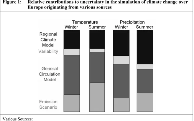
Figure 1 illustrates the relative contribution of different emission scenarios, use of different General Circulation Models (GCMs), internal GCM variability, and use of different regional climate models (RCM) to overall uncertainty in climate simulations. Although figure 1 is for Europe, it is included here to demonstrate that there are different sources of uncertainty in projecting climate change, a fact that holds true for any region in the world.

No similar figure is available for Africa. Impacts of climate change (see Section 3), de- pend strongly on local conditions. Impact assessments are thus dependent on accurate regional climate projections (see Section 2.3), which adds another source of uncertainty. The uncertainties in the different stages of climate projections (emission scenarios => climate projection => regional climate projection) complicate projections of climate change as

(14)

well as of climate impacts. Nonetheless, climate change projections are indispensable in managing global change impacts through adaptation and mitigation, provided their limita- tions are understood and considered.

2.1 Common emission scenarios

Climate change is mainly driven by emissions of greenhouse gases (GHGs), aerosol concentrations and land-use change. To study the impact on the global climate system, GCMs are driven by scenarios on GHG emissions and also aerosols. Land-use change scenarios are often included in the form of CO2 emissions only; more recently, GCMs have also at- tempted to account for changes in land surface properties (e. g. vegetation cover). All emission scenarios include assumptions on regional development and are globally consis- tent.

Figure 1: Relative contributions to uncertainty in the simulation of climate change over Europe originating from various sources

Various Sources:

1. Use of different Regional Climate Models (RCMs, 8 models);

2. internal variability of General Circulation Models (GCMs);

3. use of different GCMs (4 models);

4. use of different emission scenarios (2 scenarios covering about half the range of the Intergovernmen- tal Panel on Climate Change (IPCC) models). Winter is December, January, February; summer is June, July, August.

Uncertainty due to GCMs and scenarios (when accounting for the reduced range considered) generally dominates, except for summer precipitation, when uncertainty due to RCMs is of comparable magnitude.

Source: Giorgi (2006), modified.

Note: A coloured version of this Figure is available at http://www.die-gdi.de (publications).

(15)

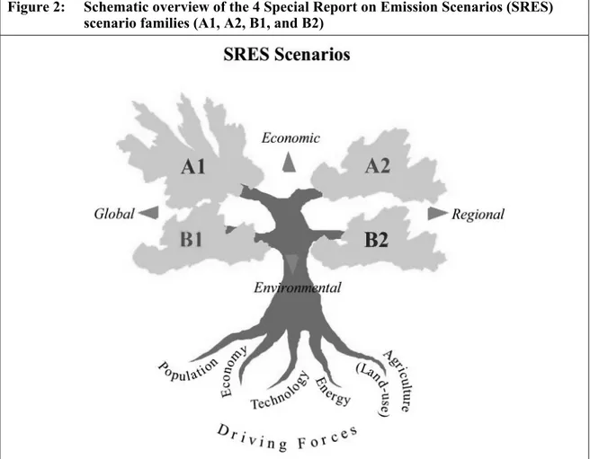
The most common emission scenarios are the so-called “SRES” scenario families, as pub- lished in the “Special Report on Emission Scenarios” (SRES) by the Intergovernmental Panel on Climate Change (IPCC) (Nakicenovic / Swart 2000). The SRES scenarios com- bine plausible assumptions on population growth, economic growth, energy use, fuel mix, and land-use change (illustrated as roots in Figure 2) and calculate CO2 emissions over the 21st century with the help of 6 different integrated assessment models (Nakicenovic/Swart 2000). Table 1 summarizes the main characteristics of the most important SRES scenarios.

The A1 and B1 scenarios assume low population growth and strong economic development, while the A2 and B2 scenarios assume higher population growth and only medium economic development. The “B” families, environmentally oriented scenarios, assume medium and low energy consumption, while the “A” families assume energy consumption to be high. Energy consumption and the choice of energy source (row 7, “favouring”) largely determine the development of CO2 emissions. Note the marked differences between A1T¹ and the other A1 scenarios as well as between the “B” scenarios and the “A”

scenarios (except A1T).

1 A sub-scenario with emphasis on technological change and renewable energies.

Figure 2: Schematic overview of the 4 Special Report on Emission Scenarios (SRES) scenario families (A1, A2, B1, and B2)

The “A” families have a general economic preference, while the “B” families are more environmentally oriented. The “1” families assume a globalized world, while the “2” families assume a regionalized world.

The roots of the tree illustrate the basic assumptions driving the scenarios.

Source: Nakicenovic / Swart (2000)

Note: A coloured version is available at http://www.die-gdi.de (publications).

(16)

Several other, more recent scenarios have been developed, for instance in the Millennium Ecosystem Assessment (Millennium Ecosystem Assessment 2005), but none have been implemented in global integrated assessment models in a manner comparable to the im- plementation of the SRES scenarios. These are therefore often only available as verbal storylines, and they are seldom used in impact studies.

2.2 Climate models

General Circulation Models (GCMs) simulate the dynamics of the atmosphere, including the transport of heat and water. Usually GCMs are coupled to a model of oceanic circulation (Atmosphere-Ocean General Circulation Model, AOGCM), since lateral and vertical

2 Resource availability of conventional and unconventional oil and gas.

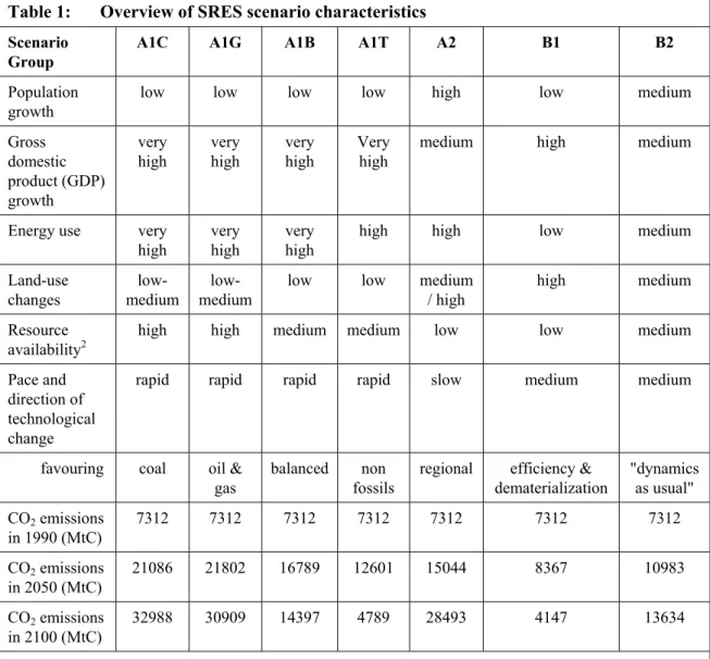
Table 1: Overview of SRES scenario characteristics Scenario

Group

A1C A1G A1B A1T A2 B1 B2

Population growth

low low low low high low medium

Gross domestic product (GDP) growth

very high

Very high

medium high medium

Energy use very high

very high

high high low medium

Land-use changes

low- medium

low low medium

/ high

high medium Resource

availability²

high high medium medium low low medium

Pace and direction of technological change

rapid rapid rapid rapid slow medium medium

favouring coal oil &

gas

balanced non fossils

regional efficiency &

dematerialization

"dynamics as usual"

CO2 emissions in 1990 (MtC)

7312 7312 7312 7312 7312 7312 7312

21086 21802 16789 12601 15044 8367 10983

32988 30909 14397 4789 28493 4147 13634

Depending on variations of some scenario assumptions, there are several sub-scenarios for the four main scenarios A1, A2, B1, and B2. Not all sub-scenarios are shown here.

Source: Nakicenovic / Swart (2000)

(17)

transport of heat in the oceans strongly affects the energy budget in the atmosphere. Land- surface properties are usually partially modelled (e. g. evapo-transpiration) and partially prescribed (e. g. vegetation cover). Recently, GCMs have sought to include full land-surface dynamics.

A broad range of climate models exist (see Table 2 for an overview of the IPCC GCMs);

most of these are AOGCMs, the most comprehensive climate models available. The most important characteristics of GCMs are the resolution of the atmosphere and of the ocean, the detail of sea-ice and land surface modelling, and flux adjustments between atmosphere, ocean, and land. Table 2 shows these main characteristics for all 23 IPCC GCMs.

The atmosphere is usually represented by different horizontal layers, defined not by specific altitudes but by pressure levels, which is more dynamic and thus more accurate. The top of the atmosphere is not a sharp border and needs to be defined in models. Most models do this via pressure levels. The lower the top pressure in the model is (ranging from 0.05 to 25 hPa), the more of the atmosphere is actually modelled. Only a few models pre- scribe the top of the atmosphere in altitude (km). Most climate models describe the motion of the atmosphere via a set of wave functions, which also determine spatial resolution via triangular spectral truncation level.³ Atmospheric horizontal resolution is expressed either as degrees latitude by longitude or as a triangular (T) spectral truncation with a rough translation to degrees latitude and longitude, ranging from 1.1° x 1.1° to 4.0° x 5.0°. Ver- tical resolution (L) is the number of vertical levels, ranging from 12 to 56 layers. Oceanic horizontal resolution is expressed as degrees latitude by longitude, while vertical resolution (L) is the number of vertical levels. Rigid lid ocean models do not move under atmospheric momentum but translate it into fluid pressure. Flux adjustments are sometimes needed to avoid unrealistic model drifts (i. e. moving slowly into unrealistic states); these are employed by only 6 of the 23 GCMs presented in Table 2. The representation of land in GCMs is largely uniform, almost all models simulate several soil-water layers (except 4) and channel surface runoff via a river routing system to the oceans (except 3), all models include a vegetation canopy, which usually is prescribed and does not react to simulated climate.

AOGCMs are very expensive in computational terms and thus can be applied only to a limited number of scenarios. Strongly reduced, so-called simple climate models are employed to assess probabilistic distributions of climate projections (Harvey et al. 1997), but they provide only insights for global-scale questions. A class of intermediate climate models, so-called EMICs (Earth System Models of Intermediate Complexity), have evolved between AOGCMs and simple climate models (Claussen et al. 2002).

Climate projections are subject to considerable uncertainty, due to emission scenarios (see Section 2.1) and GCM simulations. While all climate models have their individual strengths

3 The so-called spectral conversion transforms the complex mathematical equations describing the 3- dimensional motion of the atmosphere into more simple wave functions via a Fourier Transformation.

The precision with which these complex functions are represented in wave function sets depends on the number of wave functions included. The more wave functions are used to represent a complex function, the higher are the computational demands. Therefore, the precision of the model is usually truncated at a specific level (e. g. T42). The truncation point also determines the spatial resolution of the model, which is dependent on the density of wave nodes. A model with a high truncation point (e. g. T106 as model 18 “MIROC3.2(hires)” in Table 2) therefore has a relatively fine spatial resolution but also very high computational demands.

(18)

Model ID, Vintage

Sponsor(s), Country

Atmosphere Top Resolution⁴

Ocean Resolution⁵Z Coord., Top BC

Sea Ice Dynamics, Leads

Coupling Flux Adjustments

Land Soil, Plants, Routing 1: BCC-CM1,

2005

(Xu et al. 2005)

Beijing Climate Center, China

top = 25 hPa T63 (1.9° x 1.9°) L16

1.9° x 1.9°

L30 depth, free surface

no rheology or leads

heat, momentum

layers, canopy, routing

2: BCCR- BCM2.0, 2005 (Furevik et al.

2003)

Bjerknes Centre for Climate Research, Norway

top = 10 hPa T63 (1.9° x 1.9°) L31

0.5°–1.5° x 1.5° L35 density, free surface

rheology, leads

no

adjustments

3: CCSM3, 2005

(Collins et al.

2006)

National Center for

Atmospheric Research, USA

top = 2.2 hPa T85 (1.4° x 1.4°) L26

0.3°–1° x 1°

rheology, leads

no

adjustments

4: CGCM3.1 (T47), 2005 (Flato 2005)

Canadian Centre for Climate Modelling and Analysis, Canada

top = 1 hPa T47 (~2.8° x 2.8°) L31

1.9° x 1.9°

L29 depth, rigid lid

rheology, leads

heat, freshwater

5: CGCM3.1 (T63), 2005 (Flato 2005)

Canadian Centre for Climate Modelling and Analysis, Canada

top = 1 hPa T63 (~1.9° x 1.9°) L31

0.9° x 1.4°

rheology, leads

heat, freshwater

6: CNRM-CM3, 2004

(Deque et al.

1994)

Météo-France/

Centre National de Recherches Météorolo- giques, France

top = 0.05 hPa

T63 (~1.9° x 1.9°) L45

0.5°–2° x 2°

rheology, leads

no

adjustments

7: CSIRO- MK3.0, 2001 (Gordon et al.

2002)

Commonwealth Scientific and Industrial Research Organisation (CSIRO) Atmospheric Research, Australia

top = 4.5 hPa T63 (~1.9° x 1.9°) L18

0.8° x 1.9°

rheology, leads

no

adjustments

layers, canopy

4 Horizontal resolution is expressed either in degrees latitude by longitude or as a triangular (T) spectral truncation with a rough translation to degrees latitude and longitude. Vertical resolution (L) is the number of vertical levels.

5 Horizontal resolution is expressed as degrees latitude by longitude, while vertical resolution (L) is the number of vertical levels.

Table 2: Selected model features of the AOGCMs

(19)

Model ID, Vintage

Sponsor(s), Country

Land Soil, Plants, Routing 8: ECHAM5/

MPI-OM, 2005 (Jungclaus et al.

2006)

Max Planck Institute for Meteorology, Germany

top = 10 hPa T63 (~1.9° x 1.9°) L31

1.5° x 1.5°

rheology, leads

no

adjustments

bucket, canopy, routing

9: ECHO-G, 1999 (Min et al.

2005)

Meteorological Institute of the University of Bonn,

Meteorological Research Institute of the Korea

Meteorological Administration (KMA), and Model and Data Group,

Germany/Korea

top = 10 hPa T30 (~3.9° x 3.9°) L19

0.5°–2.8° x 2.8° L20 depth, free surface

rheology, leads

heat, freshwater

10: FGOALS- g1.0, 2004 (Wang et al.

2004)

National Key Laboratory of Numerical Modelling for Atmospheric Sciences and Geophysical Fluid Dynamics (LASG)/Institute of Atmospheric Physics, China

top = 2.2 hPa T42 (~2.8° x 2.8°) L26

1.0° x 1.0°

L16 eta, free surface

rheology, leads

no

adjustments

11: GFDL- CM2.0, 2005 (Delworth et al.

2006)

U.S. Department of Commerce/

National Oceanic and Atmospheric Administration (NOAA)/Geo- physical Fluid Dynamics Labo- ratory (GFDL), USA

top = 3 hPa 2.0° x 2.5°

L24

0.3°–1.0° x 1.0°

depth, free surface

rheology, leads

no

adjustments

12: GFDL- CM2.1, 2005 (Delworth et al.

2006)

U.S. Department of Commerce/

National Oceanic and Atmospheric Administration (NOAA)/Geo- physical Fluid Dynamics Labo- ratory (GFDL), USA

top = 3 hPa 2.0° x 2.5°

L24 with semi- Lagrangian transports

0.3°–1.0° x 1.0°

depth, free surface

rheology, leads

no

adjustments

(20)

Model ID, Vintage

Sponsor(s), Country

Land Soil, Plants, Routing 13: GISS-AOM,

2004

(Russell 2005)

National Aeronautics and Space Administration (NASA)/

Goddard Institute for Space Studies (GISS), USA

top = 10 hPa 3° x 4° L12

3° x 4° L16 mass/area, free surface

rheology, leads

no

adjustments

14: GISS-EH, 2004

(Schmidt et al.

2006)

National Aeronautics and Space Administration (NASA)/

Goddard Institute for Space Studies (GISS), USA

top = 0.1 hPa 4° x 5° L20

2° x 2° L16 density, free surface

rheology, leads

no

adjustments

15: GISS-ER, 2004

(Schmidt et al.

2006)

National Aeronautics and Space Administration (NASA)/Goddar d Institute for Space Studies (GISS), USA

top = 0.1 hPa 4° x 5° L20

4° x 5° L13 mass/area, free surface

rheology, leads

no

adjustments

16: INM- CM3.0, 2004 (Volodin/Dians ky 2004)

Institute for Numerical Mathematics, Russia

top = 10 hPa 4° x 5° L21

2° x 2.5° L33 sigma, rigid lid

no rheology or leads

regional freshwater

layers, canopy, no routing 17: IPSL-CM4,

2005

(Hourdin et al.

2006)

Institut Pierre Simon Laplace, France

top = 4 hPa 2.5° x 3.75°

L19

2° x 2° L31 depth, free surface

rheology, leads

no

adjustments

18: MIROC3.2 (hires), 2004 (K-1 model developers 2004)

Center for Climate System Research (University of Tokyo), National Institute for Environmental Studies, and Frontier Re- search Center for Global Change (JAMSTEC), Japan

top = 40 km T106 (~1.1°

x 1.1°) L56

0.2° x 0.3°

L47

sigma/depth, free surface

rheology, leads

no

adjustments

(21)

Model ID, Vintage

Sponsor(s), Country

Land Soil, Plants, Routing 19: MIROC3.2

(medres), 2004 (K-1 model developers 2004)

Center for Climate System Research (University of Tokyo), National Institute for Environmental Studies, and Frontier Re- search Center for Global Change (JAMSTEC), Japan

top = 30 km T42 (~2.8° x 2.8°) L20

0.5°–1.4° x 1.4° L43 sigma/depth, free

surface

rheology, leads

no

adjustments

20: MRI-CGCM 2.3.2, 2003 (Yukimoto/Noda 2003)

Meteorological Research Institute, Japan

top = 0.4 hPa T42 (~2.8° x 2.8°) L30

.5°–2.0° x 2.5° L23 depth, rigid lid

free drift, leads

heat, freshwater, momentum (12°S–12°N)

layers, canopy, routing 21: PCM, 1998

(Kiehl et al.

1998)

National Center for Atmospheric Research, USA

top = 2.2 hPa T42 (~2.8° x 2.8°) L26

0.5°–0.7° x 1.1° L40 depth, free surface

rheology, leads

no

adjustments

layers, canopy, no routing 22: UKMO-

HadCM3, 1997 (Cox et al.

1999)

UKMO- HadGEM1, 2004 (Martin et al. 2004)

Hadley Centre for Climate Prediction and Research/Met Office, UK Hadley Centre for Climate Prediction and Research/Met Office, UK

top = 5 hPa 2.5° x 3.75°

L19 Top = 39.2 km

~1.3° x 1.9°

L38

1.25° x 1.25°

L20 depth, rigid lid 0.3°–1.0° x 1.0° L40 depth, free surface

free drift, leads

rheology, leads

no

adjustments

no

adjustments

layers, canopy, routing layers, canopy, routing

Selected model features of the AOGCMs participating in the Coupled Model Intercomparison Project Phase 3 (CMIP3) at the Program for Climate Model Diagnosis and Intercomparison (PCMDI) are listed by IPCC identi- fication (ID) along with the calendar year (‘vintage’) of the first publication of results from each model. Also listed are the respective sponsoring institutions, the pressure at the top of the atmospheric model, the horizontal and vertical resolution of the model atmosphere and ocean models, as well as the oceanic vertical coordinate type (Z) and upper boundary condition (BC: free surface or rigid lid). Also listed are the characteristics of sea ice dynamics/structure (e.g. rheology vs. ‘free drift’ assumption and inclusion of ice leads) and whether adjustments of surface momentum, heat or freshwater fluxes are applied in coupling the atmosphere, ocean and sea ice com- ponents. Land features such as the representation of soil moisture (single-layer ‘bucket’ vs. multilayered scheme) and the presence of a vegetation canopy or a river routing scheme also are noted.

Source: Randall et al. (2007)

(22)

and weaknesses, there are some general GCM performance characteristics. Global annual mean temperatures of the 20th century are simulated reasonably well by all GCMs, especially in the northern hemisphere, while precipitation and cloud cover, both important inputs for impact models (agriculture, vegetation, hydrology), are less well reproduced by the GCMs (see Figure 3). Regionally or locally, GCMs perform less accurately, with local temperature deviations of several degrees and strong distortions of precipitation patterns.

A detailed overview of GCM performance and evaluation is given by Gleckler et al.

(2008) and Randall et al. (2007).

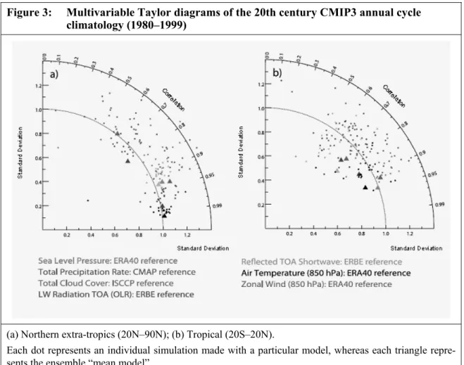
Figure 3: Multivariable Taylor diagrams of the 20th century CMIP3 annual cycle climatology (1980–1999)

(a) Northern extra-tropics (20N–90N); (b) Tropical (20S–20N).

Each dot represents an individual simulation made with a particular model, whereas each triangle represents the ensemble “mean model”.

Source: Gleckler et al. (2008).

Note: A coloured version of this Figure is available at http://www.die-gdi.de (publications).

The quality of climate simulations is very hard to assess, due to its complexity. In princi- ple, there are several criteria that need to be considered in assessing the quality of a climate simulation: the overall bias⁶ of the simulation (Is the global average too dry/wet or hot/cold etc.?), the variation of the pattern (Are extremes represented well?), the correlation of the pattern (Are dry/wet areas where dry/wet area are being observed or are they somewhere else?), and the total error (i. e. some aggregate⁷ of the total disagreement).

6 A bias in climate simulations is the deviation of the average from observations. If the simulated temperature (precipitation) is higher/lower than observations, the model has a warm/cool (wet/dry) bias.

7 Usually the root square mean error is used.

(23)

This is becoming even more complicated since these criteria have to be evaluated for a broad range of variables⁸ and should also reflect their temporal dynamics.

Gleckler et al. (2008) provide a range of performance metrics for climate models; these are still difficult to understand for persons outside the climate modeller community and are thus not shown here. Figure 3 shows so-called Taylor Diagrams (Taylor 2001), which make it possible to represent the correlation and standard deviation of several variables (distinguished by colours) and several models within one single graph. Each variable is normalized by the corresponding standard deviation of the reference data, which allows multiple variables to be shown in each panel of Figure 3. As a consequence of this normalization, the observation is located at a standard deviation of 1.0 and a correlation of 1.0. In this figure, each coloured dot represents an individual simulation made with a particular model, whereas each triangle represents the ensemble “mean model.”⁹ A perfect match of observations would in this case¹⁰ have a standard deviation and a correlation of 1.0. The values here refer to annual mean values, i. e. they exclude temporal dynamics.

The ability of GCMs to simulate specific variables better than others can be seen in Figure 3: In a (northern hemisphere), temperature simulations (black) resemble observations remarkably closely (except for a few outliers, correlation of >0.95, standard deviation between 0.9 and 1.1), while precipitation (red) is resembled less accurately (correlation of

<0.8 and a standard deviation between 0.9 and 1.2). Comparing panels a) and b) shows that temperature simulations are much more accurate for the northern extra-tropics than for the tropics. An evaluation of models for the southern extra-tropics is not provided by Gleckler et al. (2008), since reference data sets (observation-based data) are generally of poorer quality for the southern hemisphere. It should be noted that temperature observations are the most reliable reference data sets. There are several precipitation observation data sets available, and they differ considerably. Generally, the data quality for observed climate is limited in Africa due to the low density of meteorological observation stations. See, for example, the network of temperature stations (Figure 4). Note that many stations in Africa are no longer active (small dots).

2.3 Regional climate change projections for Africa 2.3.1 GCM performance for Africa

Christensen et al. (2007) review the IPCC climate models’ skills in reproducing present and past climates and also evaluating projections of temperature, precipitation, and extreme events. The main findings are summarized here.

8 These include temperature, precipitation, cloud cover, air pressure, wind speed, and short- and long- wave radiation.

9 The “mean model” statistics are calculated after regridding each model’s output to a common (T42) grid (~2.8° x 2.8°), and then computing the multimodel mean value at each grid cell.

10 This is true only because of the normalization by the corresponding standard deviation of the observed data. Otherwise, the reference data would have a standard deviation of not necessarily the 1.0 that should be most closely represented by the models.

(24)

Figure 4: Global climate network temperature stations The length of the station record is distinguished by colours. Note that many stations in Africa are no longer active (small dots). Source: http://www.globalwarmingart.com/wiki/Image: GHCN_Temperature_Stations_png by RA Rohde, based on Peterson/Vose (1997) Note: The coloured figure is part of the online version of this Discussion Paper. See: http://www.die-gdi.de (publications).

(25)

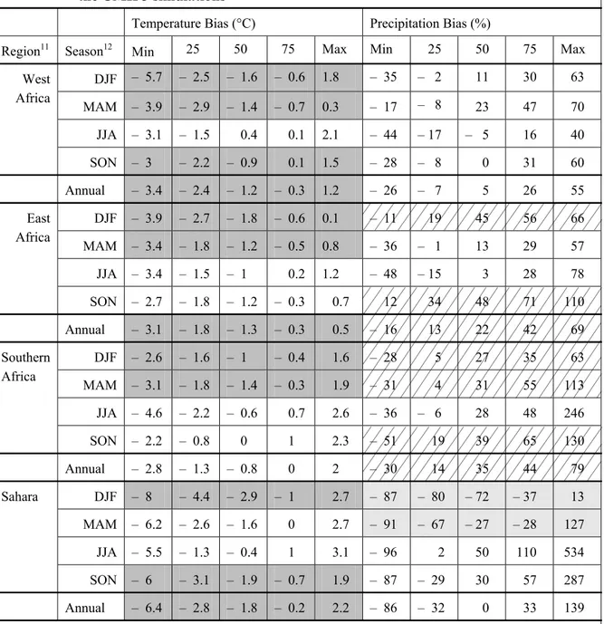
Compared to temperature observations, almost all GCMs underestimate temperatures in Africa, on average, by 1.3° C (Table 3), i. e. GCM simulations are on average too cool compared to observations. Climate modellers consider this bias to be acceptable, i. e. it does not reduce the credibility of the model’s simulations (Christensen et al. 2007, 867).

Table 3 shows that temperature biases in GCM simulations of 1980–1999 average annual temperature vary between an underestimation of 6.4°C in the Sahara to an overestimation of 2.2° C. However, 50 % of all GCMs (i. e. 2nd and 3rd quartile, see columns 25, 50, and 75 in Table 3) underestimate temperatures in all 4 African regions, range between –2.8° C and 0° C. The uniformity of the models’ bias is also illustrated by the purple shading in Table 3, indicating that at least 75 % of all models have a cool bias.

Precipitation biases of the GCMs are less uniform than temperature biases, ranging between an underestimation of annual precipitation by 86 % and an overestimation by 139 %. It should be noted that these extremes occur in the Sahara region (between 18° and 30° north and 20° and 65° east), where precipitation is low anyway, which indicates that high percentage deviations are not necessarily related to high absolute deviations. How- ever, the 3 other African Regions with higher total annual precipitation still display strong precipitation biases, ranging from underestimations of annual precipitation by 30 % over- estimates of 79 %. Especially Southern Africa (between 12° and 35° south and between 20° and 65° east), but also East Africa (between 18° north and 12° south and between 22°

and 52° east) are simulated with a wet bias by at least 75 % of the GCMs, which is indi- cated by the light blue shading in Table 3.

The evaluation of seasonal temperatures and precipitation simulations typically considers units of 3 months only (December, January, and February (DJF); March, April, and May (MAM); June, July, and August (JJA); and September, October, and November (SON).

This is insufficient to assess the GCMs’ suitability to drive specific impact models such as agricultural models, where the length of the wet season and the rainfall distribution during the wet season is crucial. There are some assessments of specific GCMs’ abilities to reproduce rainy seasons, using aggregates of 3–5 months to represent typical rainy seasons (e. g. December, January, and February for the southwest African rainy season or Febru- ary to May for East Africa rainy season (Marengo et al. 2003), also specifically for South Africa (Zhao / Camberlin / Richard 2005), but these still operate on monthly units, and a more general overview of GCMs’ abilities to reproduce rainy seasons is missing. Gener- ally, sea surface temperatures (SSTs) strongly affect the circulation patterns and thus precipitation patterns over the African continent. There is a strong relationship between the West African monsoon, precipitation in the Sahel zone and SSTs (Lenton et al. 2008) and also between Indian Ocean SSTs and southern African precipitation (Funk et al. 2008).

AOGCMs, however, have difficulties in representing the inter-annual variability of SSTs in this region, which shows in a stronger deviation of precipitation simulations from observations.

Temperature extremes are surprisingly well represented in GCM simulations, both in statistics and trend, given their coarse resolution and their large-scale systematic errors. Pre- cipitation amounts and especially intensities are less well simulated (Randall et al. 2007):

Typically, AOGCMs simulate too many days with light precipitation (<10 mm/day) and too few with heavy precipitation events. These errors partially cancel each other out in the

(26)

The simulated temperatures are compared with the HadCRUT2v (Jones et al. 2001) data set and precipitation with the CMAP (update of Xie / Arkin 1997) data set. Temperature biases are represented in °C and precipitation biases in per cent. What is shown are the minimum, median (50 %) and maximum biases among the models, as well as the first (25 %) and third (75 %) quartile values. Colours indicate regions/seasons for which at least 75 % of the models have the same sign of bias, with dark grey indicating negative temperature biases and hatching signalling positive and light grey pointing to negative precipitation biases.

Source: Christensen et al. (2007) Note: A coloured version is available at http://www.die-gdi.de

11 Regions are defined by geographic extent, see also Figure 5: West Africa: 22°N to 12°S and 20°W to 18°E, East Africa: 18°N to 12°S and 22 to 52°E, Southern Africa: 12 to 35°S and 10 to 52°E, Sahara: 18 to 30°N and 20 to 65°E.

12 Seasons are: December, January, February (DJF); March, April, May (MAM); June, July, August (JJA);

September, October, November (SON), more regional specific definitions of seasons (e. g. rainy seasons) are not typically provided and would have to be computed individually for all GCMs.

Table 3: Biases in present-day (1980–1999) surface air temperature and precipitation in the CMIP3 simulations

Temperature Bias (°C) Precipitation Bias (%)

Region¹¹ Season¹² Min 25 50 75 Max Min 25 50 75 Max DJF – 5.7 – 2.5 – 1.6 – 0.6 1.8 – 35 – 2 11 30 63 MAM – 3.9 – 2.9 – 1.4 – 0.7 0.3 – 17 – 8 23 47 70

JJA – 3.1 – 1.5 0.4 0.1 2.1 – 44 – 17 – 5 16 40 West

Africa

SON – 3 – 2.2 – 0.9 0.1 1.5 – 28 – 8 0 31 60 Annual – 3.4 – 2.4 – 1.2 – 0.3 1.2 – 26 – 7 5 26 55 DJF – 3.9 – 2.7 – 1.8 – 0.6 0.1 – 11 19 45 56 66 MAM – 3.4 – 1.8 – 1.2 – 0.5 0.8 – 36 – 1 13 29 57 JJA – 3.4 – 1.5 – 1 0.2 1.2 – 48 – 15 3 28 78 East

Africa

SON – 2.7 – 1.8 – 1.2 – 0.3 0.7 12 34 48 71 110 Annual – 3.1 – 1.8 – 1.3 – 0.3 0.5 – 16 13 22 42 69 DJF – 2.6 – 1.6 – 1 – 0.4 1.6 – 28 5 27 35 63 MAM – 3.1 – 1.8 – 1.4 – 0.3 1.9 – 31 4 31 55 113 JJA – 4.6 – 2.2 – 0.6 0.7 2.6 – 36 – 6 28 48 246 Southern

Africa

SON – 2.2 – 0.8 0 1 2.3 – 51 19 39 65 130 Annual – 2.8 – 1.3 – 0.8 0 2 – 30 14 35 44 79 DJF – 8 – 4.4 – 2.9 – 1 2.7 – 87 – 80 – 72 – 37 13 MAM – 6.2 – 2.6 – 1.6 0 2.7 – 91 – 67 – 27 – 28 127 JJA – 5.5 – 1.3 – 0.4 1 3.1 – 96 2 50 110 534 Sahara

SON – 6 – 3.1 – 1.9 – 0.7 1.9 – 87 – 29 30 57 287 Annual – 6.4 – 2.8 – 1.8 – 0.2 2.2 – 86 – 32 0 33 139