Improved electron reconstruction in ATLAS using the Gaussian Sum Filter-based model for bremsstrahlung

(1)

ATLAS-CONF-2012-047 18May2012

ATLAS NOTE

ATLAS-CONF-2012-047

May 18, 2012

Improved electron reconstruction in ATLAS using the Gaussian Sum Filter-based model for bremsstrahlung

The ATLAS Collaboration

Abstract

The behavior of high-energy electrons in the ATLAS Inner Detector is dominated by ra- diative energy losses (bremsstrahlung) as they traverse matter. These can be significant con- sidering the substantial amount of material that the Inner Detector contains and can give rise to deviations from the original charged particle’s path as it propagates through the magnetic field. As a result, significant inefficiencies, both during the electron trajectory reconstruc- tion and in the determination of the corresponding track parameters in the bending plane, can be observed. In this note, we present a modification of the electron reconstruction in ATLAS that uses track refitting with the Gaussian Sum Filter (GSF) algorithm, with the aim of improving the estimated electron track parameters. The performance of this new scheme is compared to that of the existing standard electron reconstruction, for electron transverse energies between 7 GeV and 80 GeV.

c

Reproduction of this article or parts of it is allowed as specified in the CC-BY-3.0 license.

(2)

1 Introduction

An electron can lose a significant amount of its initial energy due to bremsstrahlung energy losses when interacting with the material it traverses. This is particularly relevant with modern tracking detector designs, based on semiconductor technologies developed for optimal performance in stringent environ- ments such as those at the LHC. Such tracking detectors are characterized by non-uniformly distributed material with high concentrations at specific radial positions. While the detector elements themselves contribute very little to the overall material budget, the requirements for on-detector electronics, power distribution, cooling and mechanical support add significantly to it. Because of the electron’s small mass, radiative losses can be substantial, resulting in alterations of the curvature of the electron’s trajectory when it propagates through a magnetic field and hence of the electron track.

The ATLAS [1] Inner Detector allows the measurement of the trajectories of charged particles over five units in pseudorapidity,

|η| <

2.5, as well as the determination of their production vertices. It comprises three sub-systems: a silicon Pixel Detector at low radius providing three space points per track, a Semiconductor Tracker (SCT) providing four measurements in two stereo coordinates and a Transition Radiation Tracker (TRT) providing track-following and electron identification capability up to

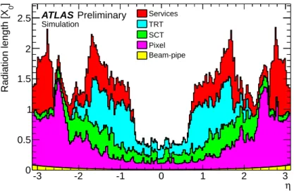
|η| =

2.0. The whole tracker is surrounded by a solenoidal magnet with a central field of 2 T. The overall material distribution of the ATLAS Inner Detector is shown in Fig. 1, illustrating significant increases at higher pseudorapidities.

The electron reconstruction scheme used for the 2010 and 2011 publications of ATLAS results em- ploys the same tracking algorithm for all charged particles, with all tracks fitted using a pion particle hypothesis to estimate the material e

ff

ects. The lack of special treatment for bremsstrahlung e

ff

ects re- sults in inefficiencies in reconstructing the electron trajectory. It also results in the degradation of the estimated track parameters, increasing with the amount of material encountered. This has a strong de- pendence on the electron pseudorapidity. By taking into account bremsstrahlung losses (and the resulting alteration of the track curvature) by using the Gaussian Sum Filter (GSF) [2, 3] approach, the estimated electron track parameters are expected to be improved.

-3 -2 -1 0 1 2 3η

] 0Radiation length [X

0 0.5 1 1.5 2

2.5 ^Services

TRT SCT Pixel Beam-pipe

ATLAS Preliminary Simulation

Figure 1:

Distribution of the Inner Detector material thickness given separately for each sub-detector as a function of the pseudorapidityη reflecting the Inner Detector description implemented in the current ATLAS simulation.

The material of the Pixel and SCT detectors include the passive material mostly located behind the active silicon sensors. The track-refitting technique presented in this note has been developed primarily to account for the radiative energy losses due to this material.

(3)

A two-step programme is underway in ATLAS to improve electron reconstruction: first to correct all track parameters associated to electron candidates by performing bremsstrahlung refitting prior to electron reconstruction and identification, and eventually to perform bremsstrahlung recovery at the ini- tial step of the electron trajectory formation to allow for more efficient track reconstruction. Correcting for bremsstrahlung e

ff

ects will also mean that track-to-calorimeter matching will use a better defined track, the electron four-momentum vector will be better determined and particle identification tools will benefit from those improvements. Such a procedure would eventually allow for more optimal electron identification in analyses, thereby potentially recovering significant e

ffi

ciency losses, especially at low transverse momentum.

This note describes the results of the first step, namely applying, prior to electron reconstruction and identification, a bremsstrahlung refit with the GSF algorithm to tracks already associated to electron candidates. The impact on the determination of track parameters and more global combined-parameters involving the calorimeter, will be presented. In Section 2, a brief overview of the Gaussian Sum Filter approach and the new electron reconstruction scheme are presented. The e

ff

ects on the reconstructed track parameters are discussed in Section 3, and more global parameters involving the electromagnetic calorimeter are reviewed in Section 4. Finally, a specific example involving electrons with small trans- verse momenta is presented in Section 5.

2 Electron Reconstruction

Electron candidates are selected by matching reconstructed tracks to clusters formed by the energy de- posited in the electromagnetic calorimeter [4, 5]. The reconstruction of a charged-particle track in AT- LAS involves determining the particle’s trajectory in the tracker from the detector response and then estimating the track parameters that best describe it. The latter include two parameters that give the transverse (d

0

) and the longitudinal position (z

0

) of the perigee (impact parameters), two parameters that describe the direction of the charged particle at this point (φ, θ) and one parameter that provides the in- verse track momentum multiplied by the charge (q/p). The errors on the track parameters originate from experimental uncertainties due to the intrinsic resolution of the tracker sensors and the interaction of the charged particle with the detector material. The track parameters and their corresponding uncertainties are estimated from the track-fitting process. For muons or pions (neglecting hadronic interactions), an essentially linear least-squares fit using a linearized helical model with scattering angle formulation [6,7]

is used to estimate the trajectory from the set of experimental measurements. Unfortunately in the case of electrons, such an assumption is not valid since their trajectory is a

ff

ected by energy losses dominated by bremsstrahlung.

A well-known model of the energy loss of electrons due to bremsstrahlung was proposed by Bethe and Heitler [8]. According to this model, the probability density function for an electron to retain a portion z

= ^E_E^f_i

of its initial energy E

i

as its final energy E

f

, is given by [2, 8]:

f (z)

=

[−lnz]

^a−1

Γ

(a)

,

with a

=

t/ln2, 0

<

z

<

1 (1)

where t is the thickness of the material traversed by the electron in units of radiation length X

₀

. The ex-

pression above needs to be modified in order to account for processes, such as the Landau-Pomeranchuk-

Migdal (LPM) or the Ter-Mikaelian e

ff

ects, that become prominent at electron energies of the order of

several GeV or higher [9]. The resulting probability density function cannot be expressed in an analyti-

cal form, but it can be implemented numerically in simulation engines like GEANT4 [10] providing the

model that describes the radiative energy losses of electrons. Under those conditions, a non-linear fitter

may provide better estimations of the track parameters. Such a fitter, based on a generalisation of the

Kalman Filter [11], and called the Gaussian Sum Filter (GSF), has been developed in [3]. It assumes that

(4)

η -2.5 -2 -1.5 -1 -0.5 0 0.5 1 1.5 2 2.5 > True/q/p Rec< q/p

1 1.5 2 2.5 3 3.5 4

All Electrons Low Bremsstrahlung High Bremsstrahlung

ATLAS Preliminary

Simulation Without GSF

(a)

η -2.5 -2 -1.5 -1 -0.5 0 0.5 1 1.5 2 2.5 > True/q/p Rec< q/p

1 1.5 2 2.5 3 3.5 4

All Electrons Low Bremsstrahlung High Bremsstrahlung

Simulation With GSF

(b)

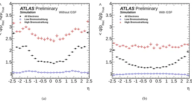
Figure 2:

Mean value of the ratio of the reconstructed over the true electron inverse momentum times charge (q/p) as a function of pseudorapidity for single electrons with transverse momentum between 7 and 80 GeV that lose less than (open points) and greater than (open triangles) 20% of their energy due to bremsstrahlung in the silicon detector and surrounding infrastructure without (a) and with (b) GSF refitting applied. Electrons that suffer significant bremsstrahlung losses dominate the high pseudorapidity regions. This explains the larger dependence with pseudorapidity when all the electrons are averaged (solid points).

the trajectory state can be approximated as a weighted sum of Gaussian functions. The GSF splits the experimental noise into individual Gaussian components and uses the Kalman filter technique in order to process each one. The GSF therefore consists of a number of Kalman filters running in parallel, each one representing a di

ff

erent contribution to the full Bethe-Heitler spectrum. In its current ATLAS imple- mentation, the Gaussian Sum Filter is used to account for the radiative loss e

ff

ects of electrons as they traverse the silicon trackers. In the case of the Transition Radiation Tracker, it has been found that due to the more homogeneous distribution of the detector material and the lower precision of the measurements, applying the GSF does not result in any appreciable improvements.

Using the GSF, all the tracks with transverse momentum p

T >

400 MeV and

|η| <

2.5 that are assigned to electrons [5] in an event can be refitted. The resulting new collection of bremsstrahlung- corrected tracks and the corresponding electromagnetic clusters form new inputs to the standard electron reconstruction algorithm. This procedure has several advantages:

1. The approach described above is expected to improve the estimation of bending-plane quantities, as is presented in more detail in Section 3. In particular, their dependence on the amount of material encountered by (and hence the pseudorapidity of) the electron should be significantly reduced as shown in Fig. 2 in the case of simulated single electrons with transverse momenta between 7-80 GeV.

2. The extrapolation of the tracks and their matching to the electromagnetic calorimeter clusters is

performed using the re-estimated track parameters. It is therefore expected that in certain cases

the track considered as the best match to the electromagnetic cluster will have changed. Some

improvements are also possible in the case of the di

ff

erent electron identification categories. This

is particularly likely in the case of the so-called “tight” electrons [4, 5] (which make use of both

first and second sampling layer calorimeter information, information from the two silicon detectors

(5)

d0

-0.1 -0.08 -0.06 -0.04 -0.02 0 0.02 0.04 0.06 0.08 0.1

Entries / 0.0025 mm

20 40 60 80 100 120 140 160 180 200 220 240

103

×

ATLASPreliminary Simulation

= 7 TeV s

ee (Standard)

→ Z

ee (GSF)

→ Z

[mm]

d0

-0.1 -0.08 -0.06 -0.04 -0.02 0 0.02 0.04 0.06 0.08 0.1

GSF/Standard ^0.7

0.8 0.9 1 1.1

(a)

0) σ(d

0/ d

-5 -4 -3 -2 -1 0 1 2 3 4 5

Entries / 0.125

0 50 100 150 200 250 300

103

×

= 7 TeV s

ee (Standard)

→ Z

ee (GSF)

→ Z

0) σ(d

0/ d

-5 -4 -3 -2 -1 0 1 2 3 4 5

GSF/Standard

0.4 0.6 0.8 1 1.2

(b)

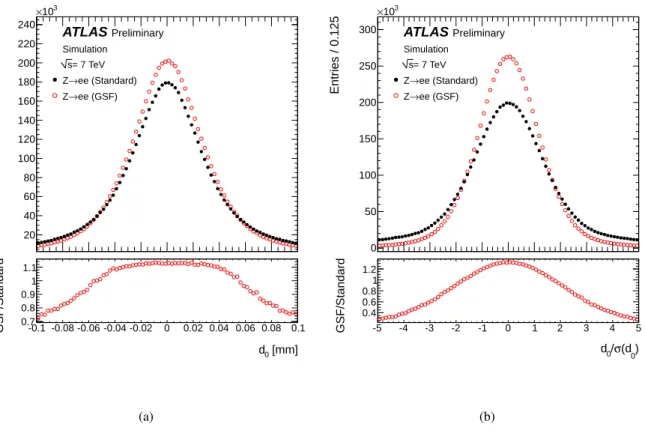
Figure 3:

The distribution of the transverse impact parameter resolution (a) and of the transverse impact parameter significance (b) for both GSF (open red) and standard (solid black) truth-matched Monte-Carlo electrons from Z-boson decays. The bottom plots show the ratio of the entries of the GSF and standard electrons per bin.

and the Transition Radiation Tracker, E/p, as well as matching between tracking and calorimeter

η

and

φ

position), where several quantities sensitive to bremsstrahlung losses are employed. The above implications are described in more detail in Section 4.

3. The electron four-momentum is computed using the improved estimates of the track parame- ters. This is particularly beneficial in the case of low-p

_T

electrons where the contribution to the resolution of the four-momentum of the track parameters is dominant and where the impact of bremsstrahlung losses is more severe. Furthermore the reconstructed invariant masses of reso- nances decaying into two electrons are also better evaluated. Both of the above are especially relevant in the case of the J/ψ resonances, where lower energy electrons are involved, as is demon- strated in Section 5.

3 Electron Track Parameters

This section focuses on presenting the improvements in the track parameters in the transverse plane. It should be noted that a full account of the radiative energy losses of an electron is practically impossible.

Although the track parameters do improve, some bias will always remain. This is especially the case if the electron has lost significant amounts of energy due to bremsstrahlung at low radius inside the ATLAS Inner Detector, e.g. in the first two Pixel Detector layers. Radiative energy losses are expected to only marginally a

ff

ect the track parameters in the longitudinal plane. For the results presented in this section when simulated data samples are presented, only reconstructed electrons that pass the “loose++” [4, 5]

selection and have been associated to the corresponding generator ones, referred to as truth-matched

(6)

[rad]

truth

φ

reco- φ

-0.005-0.004-0.003-0.002-0.001 0 0.0010.0020.0030.0040.005

Entries / 0.00012 rad

0 200 400 600 800 1000

103

×

= 7 TeV s

ee (Standard)

→ Z

ee (GSF)

→ Z

[rad]

truth

φ

reco- φ

-0.004 -0.002 0 0.002 0.004

GSF/Standard

0.6 0.8 1 1.2 1.4

(a)

truth

(q/p)

truth

-(q/p) (q/p)reco

-0.4 -0.2 0 0.2 0.4 0.6 0.8 1

Entries / 0.01875

0 100 200 300 400 500 600

103

×

= 7 TeV s

ee (Standard)

→ Z

ee (GSF)

→ Z

truth

(q/p)

truth

-(q/p) (q/p)reco

-0.4 -0.2 0 0.2 0.4 0.6 0.8 1

GSF/Standard

2 4 6 8 10

(b)

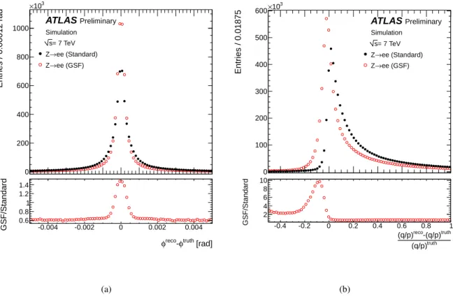
Figure 4:

The distribution of the resolution of the track directionφat the perigee (a) and of the relative bias on the track inverse momentum multiplied by the charge q/p (b), for both GSF (open red) and standard (solid black) truth-matched Monte-Carlo electrons from Z-boson decays. The bottom plots show the ratio of the entries of the GSF and standard electrons per bin.

Monte-Carlo electrons, are used.

3.1 Transverse Track Parameters Resolution

The distributions of the transverse track parameters are shown in Figs. 3 and 4 for the case of electrons

from Z-boson decays. In Fig. 3(a) the resolution of the transverse impact parameter d

₀

is shown. The

transverse impact parameter significance d

₀/σd₀

is defined as the ratio of the transverse impact parameter

d

₀

to the error from the track fitting procedure,

σd₀

, and is shown in Fig. 3(b). Fig. 4(a) shows the

resolution of the track direction

φ

at the perigee. Finally, the relative bias of the track inverse momentum

multiplied by the charge q/ p is shown in Fig. 4(b). As expected, there is a clear improvement in the

resolution of all the bending-plane track parameters when radiative losses are accounted for during the

track fitting. This could potentially have important implications in physics analyses, for example in the

Higgs-boson searches via its decay into two Z-bosons with at least one of the latter subsequently decaying

into two electrons. Here, the final-state electrons resulting from the Higgs-boson decay sequence can be

separated from those originating from heavy-quark decays by a cut on the transverse impact parameter

significance since electrons from heavy quark decay are expected to have large true d

₀

values, whereas

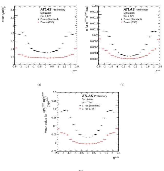
the true transverse impact parameter of electrons from Z decays should be zero. Equally important is

the dependence of the transverse track parameters resolution width (or of the mean relative bias in the

case of the track q/p) on the electron pseudorapidity

η

or transverse momentum p

_T

as shown in Figs. 5

and 6. At larger pseudorapidities, the amount of material encountered by the electron increases, resulting

in increased degradation of the reconstructed track parameters. As is evident in Fig. 5, accounting for the

(7)

truth

η -2.5 -2 -1.5 -1 -0.5 0 0.5 1 1.5 2 2.5 ) 0(dσ/0 for dσ

1 1.2 1.4 1.6 1.8 2 2.2

2.4 ATLASPreliminary Simulation

= 7 TeV s

ee (Standard)

→ Z

ee (GSF)

→ Z

(a)

truth

η -2.5 -2 -1.5 -1 -0.5 0 0.5 1 1.5 2 2.5 [rad]truth φ-reco φ for σ

0 0.0002 0.0004 0.0006 0.0008 0.001 0.0012 0.0014 0.0016 0.0018 0.002

= 7 TeV s

ee (Standard)

→ Z

ee (GSF)

→ Z

(b)

truth

η -2.5 -2 -1.5 -1 -0.5 0 0.5 1 1.5 2 2.5

truth (q/p)

truth -(q/p)reco (q/p) Mean value for

-0.05 0 0.05 0.1 0.15 0.2 0.25 0.3

= 7 TeV s

ee (Standard)

→ Z

ee (GSF)

→ Z

(c)

Figure 5:

The dependence on the pseudorapidityηof the width of the transverse impact parameter significance (a), of the width of the resolution of the track direction at the perigeeφ(b), and of the mean relative bias of the track inverse momentum multiplied by the charge q/p (c), for GSF (open red) and standard (solid black) truth-matched Monte-Carlo electrons from Z-boson decays.

bremsstrahlung losses during the track fitting reduces these e

ff

ects. In addition, the mean relative bias on the reconstructed electron track inverse momentum multiplied by the charge (q/ p) is reduced.

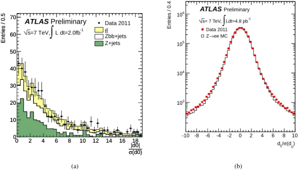
3.2 Comparison with Data for the Transverse Impact Parameter Significance

In data, electrons produced by heavy-quark or Z-boson decays can be arranged in two separate samples

and then be used to check how well the simulation describes the reconstructed transverse impact param-

eter significance when the bremsstrahlung corrections are included. Electrons from b-hadron decays are

(8)

[GeV]

truth

pT

10 15 20 25 30 35 40 45 50 55

) 0(dσ/0 for dσ

1 1.2 1.4 1.6 1.8 2 2.2

2.4 ATLASPreliminary Simulation

= 7 TeV s

ee (Standard)

→ Z

ee (GSF)

→ Z

(a)

[GeV]

truth

pT

10 15 20 25 30 35 40 45 50 55

[rad]truth φ-reco φ for σ

0 0.0002 0.0004 0.0006 0.0008 0.001 0.0012 0.0014 0.0016 0.0018 0.002

= 7 TeV s

ee (Standard)

→ Z

ee (GSF)

→ Z

(b)

[GeV]

truth

pT

10 15 20 25 30 35 40 45 50 55

truth (q/p)

truth -(q/p)reco (q/p) Mean value for

-0.05 0 0.05 0.1 0.15 0.2 0.25 0.3

= 7 TeV s

ee (Standard)

→ Z

ee (GSF)

→ Z

(c)

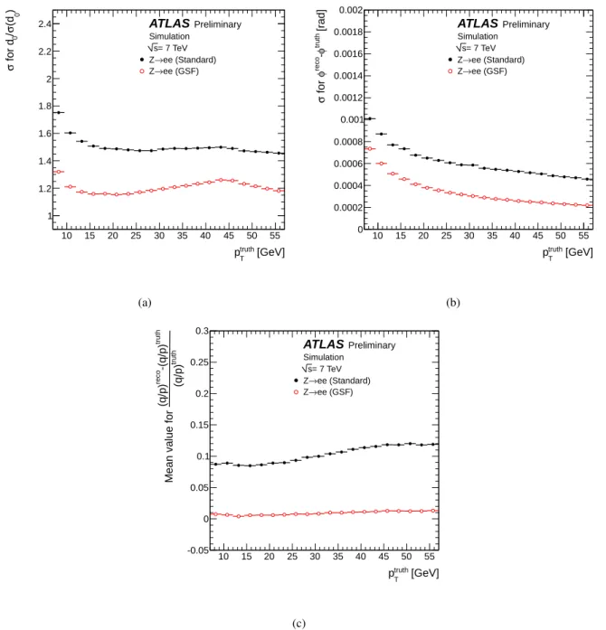
Figure 6:

The dependence on the transverse momentum pT of the width of the transverse impact parameter significance (a), of the width of the resolution of the track direction at the perigeeφ(b), and of the mean relative bias of the track inverse momentum multiplied by the charge q/p (c), for GSF (open red) and standard (solid black) truth-matched Monte-Carlo electrons from Z-boson decays.

selected in data events where either a Z-boson [12] or a t¯ t pair (through the dilepton channel [13]) has

already been identified. At least one b-tagged jet with p

_T >

25 GeV is required in the event. One can

then look for additional electrons in the selected events that have a well-reconstructed cluster matched to

a track, with p

_T >

7 GeV and

|η| <

2.47 and pass the “loose

++

” selection criteria. These electrons are

required to lie within a cone

∆

R

<

0.5 around the tagged jet. On the other hand, electrons from Z-boson

decays are identified using a tag-and-probe approach. The tag electron is an isolated electron that passes

the “tight” selection, while the probe electron is only required to pass the “loose

++

” selection, using the

criteria defined in [4, 5]. The two electrons are required to have opposite charges and to have an invariant

(9)

σ|d0|(d0)

0 2 4 6 8 10 12 14 16 18

Entries / 0.5

0 10 20 30 40 50 60 70

σ|d0|(d0)

0 2 4 6 8 10 12 14 16 18

Entries / 0.5

0 10 20 30 40 50 60 70

Data 2011 t t Zbb+jets Z+jets

L dt=2.0fb-1

∫

=7 TeV, s

(a)

0) σ(d

0/ d

-10 -8 -6 -4 -2 0 2 4 6 8 10

Entries / 0.4

103

104

105

106 ATLASPreliminary Ldt=4.8 pb-1

∫

= 7 TeV, s

Data 2011 ee MC

→ Z

(b)

Figure 7:

Comparison between data and simulation of the reconstructed transverse impact parameter significance for GSF-reconstructed electrons from heavy-quark decays (a) (where due to the limited statistics the absolute value of the transverse impact parameter significance is used instead) and from Z-boson decays (b). The small shift visible between the MC and the data distributions in the latter plot is due to a feature in the ATLAS simulation that is unrelated to the bremsstrahlung treatment studied in this note.

mass within 15 GeV from that of the Z-boson. The distribution of the reconstructed transverse impact parameter significance for electrons refitted using the GSF in data is shown in Fig. 7. The agreement between the data and the simulation is very good.

4 Electron Combined-Parameter Performance

Combined parameters are computed using the selected electron tracks as described in Section 3 and the associated calorimeter information via the track-to-calorimeter matching criteria. The ATLAS Liquid- Argon Electromagnetic Calorimeter extends to a pseudorapidity of

|η| =

3.2. Over the

|η| <

2.5 range covered by the tracker, it makes precision measurements with three sampling depths. The combined parameters discussed in this section include the calorimeter energy to track momentum ratio (E/p), and the difference in the extrapolated track impact point to the second sampling of the calorimeter

φ

cluster barycentre position (

∆φ₂

). The latter has been multiplied by the charge sign so that the impact point di

ff

erence is independent of the particle charge. They are used in the electron identification algorithms, particularly in the so-called “tight++” identification [4, 5], which makes use of both first and second sampling layer calorimeter information, information from the two silicon detectors and the Transition Radiation Tracker, E/p, as well as matching between tracking and calorimeter

η

and

φ

position.

The following subsections show comparisons of the GSF-refitted simulated electrons to the standard-

reconstructed electrons as well as comparisons between simulation and collision data of GSF-refitted

electrons from Z-boson decays. One example is also shown for prompt J/ψ

→

ee data, to illustrate the

good data to Monte Carlo agreement of GSF electrons at lower energies.

(10)

0 1 2 3 4 5 6 7 8 9 10

Entries/0.1

10-4

10-3

10-2

10-1

ATLAS Preliminary

=7 TeV s Simulation

ee MC

→ Z

Standard GSF

E/p

0 1 2 3 4 5 6 7 8 9 10

GSF/Standard

0.6 0.81 1.2 1.4 1.6 1.82

(a)

-0.1 -0.08 -0.06 -0.04 -0.02 0 0.02 0.04

Entries/0.004 rad

10-4

10-3

10-2

10-1

=7 TeV s Simulation

ee MC

→ Z

[rad]

φ2 -0.1 -0.08 -0.06 -0.04 -0.02 0 0.02∆ 0.04

GSF/Standard

0 0.5 1 1.5 2

(b)

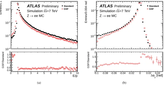
Figure 8:

The distributions of the calorimeter energy to track momentum ratio (E/p in (a)) and of the azimuthal φ difference between the extrapolated track and the corresponding cluster position as measured in the second sampling of the calorimeter (∆φ₂ in (b)), for truth-matched Monte-Carlo GSF (open red) and standard (solid black) electrons. The GSF-to-standard ratio is given below.

4.1 Combined Track-Calorimeter Parameters

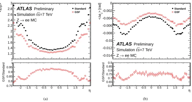
Distributions of E/ p and

∆φ2

for truth-matched simulated electrons from Z decays are shown in Fig. 8, as well as the dependence of their means on

η

in Fig. 9. The GSF-refitted electrons are better centred at E/ p

=

1 and

∆φ₂ =

0 with smaller radiative tails than the standard electrons candidates. The

η

dependence of the mean of the distributions is noticeably flattened, implying lesser sensitivity to mate- rial e

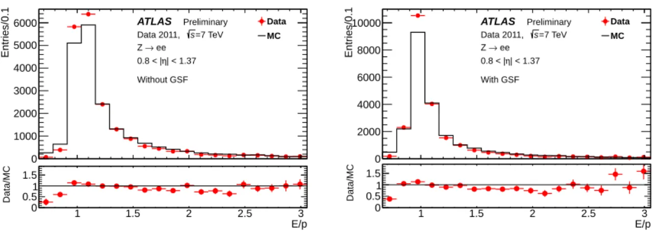
ff

ects in the case of the GSF-refitted electrons. Figure 10 illustrates the good agreement between data and simulation for the E/p variable for the case of reconstructed electrons in the electromagnetic calorimeter outer barrel (0.8

<|η|<

1.37). Figure 11 shows an equivalent plot for J/ψ

→

ee events which represent electrons with fairly low energies in the range 7 GeV< E

_T <15 GeV where, as discussed earlier

in this note, radiative energy losses are more pronounced.

4.2 Electron Identification E ffi ciencies

Since the GSF-refitted tracks and their associated calorimeter cluster information form the new input to the electron identification algorithm, electron identification e

ffi

ciencies are expected to improve. The

“tight

++

” electron identification e

ffi

ciency with respect to Monte-Carlo truth information is shown in

Fig. 12 as a function of electron

η. Electrons refitted with GSF show an improvement in the electron

identification e

ffi

ciency of over 5% at high

|η|. The improvement as a function of transverse momentum

is approximately 2% at 15 GeV and 0.5% at 70 GeV. The “tight

++

” selection requirements used in

the plots shown have been optimised for the older standard electrons. Further improvement might be

achieved by reoptimising these requirements when the new GSF-refitted tracks are used.

(11)

-2 -1.5 -1 -0.5 0 0.5 1 1.5 2

<E/p>

1 1.2 1.4 1.6 1.8 2 2.2 2.4 2.6 2.8 3

=7 TeV s Simulation

ee MC

→ Z

-2 -1.5 -1 -0.5 0 0.5 1 1.5 2 η

GSF/Standard

0.75 0.8 0.85 0.9 0.95 1

(a)

-2 -1.5 -1 -0.5 0 0.5 1 1.5 2

> [rad] 2φ∆<

-0.014 -0.012 -0.01 -0.008 -0.006 -0.004 -0.002 0

=7 TeV s Simulation

ee MC

→ Z

-2 -1.5 -1 -0.5 0 0.5 1 1.5 2 η

GSF/Standard

0.6 0.65 0.7 0.75 0.8 0.85 0.9

(b)

Figure 9:

The dependence on the pseudorapidityηof the mean calorimeter energy to track momentum ratio (E/p, in (a)) and of the mean difference of extrapolated track φ to the clusterφ position as measured in the second sampling of the calorimeter (∆φ₂ in (b)), for truth-matched Monte-Carlo GSF (open red) and standard (solid black) electrons. The GSF-to-standard ratio is given below.

4.3 Choice of Tracks Matched to Clusters

It is instructive to see how often a different track is matched to the calorimeter cluster as a result of the GSF-refitting, compared to the standard tracking. This information is shown in Fig. 13 as a function of

η.

In the central

η

region, a new track is rarely selected, but this choice is changed in approximately 5% of the cases at high

|η|. Matching to different tracks is largely independent of

p

_T

, averaging approximately 0.8% over the entire p

_T

kinematic range.

5 J/ψ Invariant Mass Shape with GSF-refitted Electrons

The greatest improvements in electron reconstruction after implementing bremsstrahlung correction

techniques are expected at low (

.

15 GeV) transverse energies. The J/ψ meson (m

J/ψ=

3069.9 MeV [14])

provides an abundant source of low energy di-electron final states, and is therefore a testbed tool for val-

idation studies of these bremsstrahlung-aware reconstruction tools. In addition to an increase in the

reconstruction and identification e

ffi

ciencies, gains in the resolution of electron kinematic quantities will

lead to improvements in the accuracy of the parent J/ψ four-vector. As a result, the position of the peak

of the parent invariant mass distribution should be more accurate, which could be important in the mea-

surement of the mass of new particles (e.g. exotic new quarkonia states). The mass resolution is also

expected to improve, which is particularly desirable for the separation of closely spaced states such as

the

Υ(1S

),

Υ(2S

) and

Υ(3S

). Other indirect benefits may also be seen in physics measurements that are

reliant on angular distributions (e.g. polarisation), or those which are sensitive to bin migrations (such as

differential cross-sections). Aside from the best-fit values for the kinematic variables, an improvement

is also expected in the covariance matrix for the four-vectors benefiting, for example, the vertex position

fits and lifetime measurements.

(12)

E/p

1 1.5 2 2.5 3

Data/MC

0 0.51 1.5

Entries/0.1

0 1000 2000 3000 4000 5000

6000 ATLAS Preliminary

=7 TeV s Data 2011,

→ ee Z

| < 1.37 η 0.8 < | Without GSF

Data MC

E/p

1 1.5 2 2.5 3

Data/MC

0 0.5 1 1.5

Entries/0.1

0 2000 4000 6000 8000

10000 ATLAS Preliminary

=7 TeV s Data 2011,

→ ee Z

| < 1.37 η 0.8 < | With GSF

Data MC

Figure 10:

Comparison of the data to a simulation of the calorimeter energy to track momentum ratio (E/p), for0.8 <|η|<1.37using standard (left plot) and GSF (right plot) tracking for Z→ ee candidate electrons with reconstructed electron energy 15 GeV<ET <25 GeV.

E/p

1 1.5 2 2.5

Data/MC

0 0.51 1.5

Entries/0.1

0 500 1000 1500 2000 2500 3000 3500 4000

4500 ATLAS Preliminary = 7 TeV s Data 2011,

→ ee ψ J/

| < 1.37 η 0.8 < | Without GSF

Data MC

E/p

1 1.5 2 2.5

Data/MC

0 0.51 1.5

Entries/0.1

0 1000 2000 3000 4000

5000 ATLAS Preliminary = 7 TeV s Data 2011,

→ ee ψ J/

| < 1.37 η 0.8 < | With GSF

Data MC

Figure 11:

Comparison of the data to a simulation of the calorimeter energy to track momentum ratio (E/p), for 0.8 <|η| <1.37using standard (left plot) and GSF (right plot) tracking for J/ψ → ee candidate electrons with reconstructed electron energy 7 GeV<ET <15 GeV.

5.1 J/ψ Candidate Selection

This study uses a Monte-Carlo data sample of about 5 million prompt J/ψ produced by the PYTHIA 6 [15]

generator (which uses the MRST LO

^∗

[16] parton distribution functions) with an ATLAS-specific tune [17].

Prompt refers to those J/ψ directly produced in the primary (hard) interaction, or from the decay of ex- cited charmonium states (e.g.

χ_c1 → γ

J/ψ). A non-prompt J/ψ sample was also initially studied, but showed similar results to the prompt sample and so is not discussed here. A subset of the full 2011 collision data-set (approximately 37 million events recorded early during the data-taking campaign and combining all contributing electron triggers) is also included in the analysis for comparison with the simulation. For both the data and simulation samples, events were processed with (1) the standard elec- tron reconstruction algorithm and (2) the modified algorithm where the GSF is used to refit all tracks associated to each electromagnetic cluster, leaving the track-cluster matching and identification criteria unchanged.

A standard candidate selection is employed, which requires two opposite-sign reconstructed elec-

trons, each with an associated track containing at least 6 silicon hits (with at least one of these in the

(13)

-2 -1.5 -1 -0.5 0 0.5 1 1.5 2

Tight efficiency

0.3 0.4 0.5 0.6 0.7 0.8 0.9 1

ATLAS Preliminary

=7 TeV s

Simulation ee MC

→ Z

-2 -1.5 -1 -0.5 0 0.5 1 1.5 2

η

GSF/Standard

0.96 0.98 1 1.02 1.04 1.06 1.08

Figure 12:

The “tight++” electron identification efficiency with respect to Monte-Carlo truth as a function ofη, for GSF (open red) and standard (solid black) electrons. The GSF-to-standard ratio is given below.

pixel detector). Both electrons are required to fulfil the “tight” electron identification criteria. For each J/ψ

→

ee decay candidate passing these selections, the two electron tracks are then fitted to a common vertex with the requirement on the fit quality that

χ²_vertexfit <

200. Precise knowledge of the position of the vertex is essential in any attempt to separate prompt from non-prompt J/ψ. The resulting vertex-refitted tracks and their corresponding covariance matrices are then used to construct the J/ψ four-vector and covariance matrix, from which the invariant mass and uncertainty (m

e⁺e⁻

and

δme⁺e⁻

, respectively) are calculated.

5.2 Results and Discussion

The invariant mass distributions for the prompt simulation sample are shown in Fig. 14(a), with the results for the standard electron reconstruction and reconstruction using GSF track fitting, normalized to the same number of entries, overlaid for comparison. The shape of the curve for the GSF-refitted electrons is much more symmetrical about its peak value, which is in addition closer to the PDG value of 3096.9 MeV [14]. A tail to the left of the peak remains due to the inability of the GSF algorithm to account for bremsstrahlung losses when the photon emission occurs very close to the electron production vertex, but as can be seen in the figure, the resolution is indeed narrower when using GSF refitting. These trends are also reflected in the results for the collision data sample (Fig. 14(b)). The distribution for the data also includes a secondary, smaller peak at the

ψ(2S

) mass, which is slightly more visible for the GSF reconstruction.

The evolution of the mass shape with the pseudorapidity of the electrons is another point of interest.

In Fig. 15(b), the invariant mass for the GSF-refitted Monte-Carlo J/ψ sample is displayed as a function

(14)

-2 -1.5 -1 -0.5 0 0.5 1 1.5 2 η

Changed track/all

0 0.01 0.02 0.03 0.04 0.05 0.06

ATLAS Preliminary

=7 TeV s

Simulation ee MC

→ Z

GSF

Figure 13:

Fraction of Monte-Carlo electron candidates for which a different track was matched to the calorimeter cluster as a result of GSF-refitting (compared to the original track selection for standard tracking) as a function of η.

of the parent J/ψ rapidity. The width of the distributions is strongly dependent on the rapidity, but the position of the peak is more stable than in the case of the standard electron reconstruction (Fig. 15(a)).

The observed poorer resolution in the forward regions is as expected, since for these trajectories there is generally more material in the detector and less coverage by the tracking elements.

To quantify the shapes of the GSF distributions, binned maximum-likelihood fits were performed using the Crystal Ball (CB) function for the signal peak and a second order Chebychev polynomial to describe the background. The intrinsic width of the mass distributions is a function of the rapidity (see Fig. 15(b)). An accurate description of the signal shape across the entire rapidity range would require several CB curves to account for this. This complication was avoided by restricting the rapidity range of the J/ψ candidates to

|y| <

0.1, where the width is essentially constant. For the collision data sample, a second CB was used to describe the

ψ(2S

) resonance. The fits for the two samples are given in Fig. 16, with values for the peak parameter m

_J/ψ

of 3105–3107 MeV, and having consistent widths.

Though the position of the mean is slightly above the PDG value (by approximately 10 MeV), it is a

clear improvement over the peak value for standard electron reconstruction, which is at approximately

3020 MeV. The widths measured in these fits using the GSF algorithm (73 and 85 MeV for simulation

and data, respectively) are much narrower compared to the results when using calorimeter measurements

of transverse energy on similar data samples (typically

&

110 MeV). For comparison, distributions for

J/ψ

→µ⁺µ⁻

decays are symmetric and have a width of about 50 MeV [18]. The success of the CB fits

here in describing the peak shape is encouraging, as it is important for accurate extraction of yields for

cross-section measurements.

(15)

[MeV]

e-

e+

m

1500 2000 2500 3000 3500 4000

Arbitrary Units / 50 MeV

0 0.02 0.04 0.06 0.08 0.1 0.12 0.14 0.16

Standard Electrons GSF-refitted Electrons Standard Electrons GSF-refitted Electrons Standard Electrons GSF-refitted Electrons

Preliminary ATLAS

Simulation = 7 TeV s

(a) PromptJ/ψMonte Carlo.

[MeV]

e-

e+

m

1500 2000 2500 3000 3500 4000

0 0.005 0.01 0.015 0.02 0.025

Data 2011 (Standard) Data 2011 (GSF) Data 2011 (Standard) Data 2011 (GSF) Data 2011 (Standard) Data 2011 (GSF) Data 2011 (Standard) Data 2011 (GSF)

= 7 TeV s

(b) 2011 collision data.

Figure 14:

The e⁺e⁻ invariant mass distributions for prompt J/ψsimulation (a) and 2011 collision data samples (b).

[MeV]

e-

e+

m

1500 2000 2500 3000 3500 4000

0 0.01 0.02 0.03 0.04 0.05 0.06 0.07 0.08 0.09 0.1

0.0<|y|<0.5 0.5<|y|<1.0 1.0<|y|<1.5 1.5<|y|<2.0 2.0<|y|<2.5

Standard electrons

(a) Standard electron reconstruction.

[MeV]

e-

e+

m

1500 2000 2500 3000 3500 4000

0 0.02 0.04 0.06 0.08 0.1 0.12 0.14 0.16 0.18

0.0 < |y| < 0.5 0.5 < |y| < 1.0 1.0 < |y| < 1.5 1.5 < |y| < 2.0 2.0 < |y| < 2.5 Preliminary ATLAS

GSF-refitted electrons

(b) GSF electron reconstruction.

Figure 15:

The invariant mass distributions as a function of the combined e⁺e⁻rapidity for the standard (a) and GSF reconstruction (b) of simulated J/ψdecays. While the widths of the distributions clearly increase in the more forwardηregions, the GSF algorithm successfully stabilises the position of the peak.

6 Summary and Conclusions

A modification of the ATLAS electron reconstruction scheme, that uses track refitting with the Gaussian

Sum Filter (GSF) algorithm to account for the e

ff

ects of bremsstrahlung, is presented in this note. It is

demonstrated that this procedure leads to an improved estimation of bending-plane quantities such as

the transverse impact parameter significance, track angular direction at the perigee

φ, and the inverse

momentum multiplied by the charge q/ p. Distributions of combined track and calorimeter parameters

such as the calorimeter energy to track momentum ratio, E/p, as well as the difference in extrapolated

track impact point to the calorimeter second sampling

φ

cluster barycentre position,

∆φ₂

, are observed to

be narrower and less dependent on the amount of material traversed by the electron, which is a function

of the electron pseudorapidity, being larger at large

|η|

. Improvements on the order of up to 5% for

electron identification efficiency at large

|η|

in the endcap regions are also demonstrated. Significant

improvements are observed in the invariant mass mean and width of J/ψ

→

ee since the electron four-

momentum is computed using the better-estimated track parameters. This note concludes the first phase

of a two-step programme in ATLAS to improve the electron reconstruction aiming at correcting all tracks

(16)

[MeV]

e-

e+

m

2000 2200 2400 2600 2800 3000 3200 3400 3600 3800 4000

0 0.02 0.04 0.06 0.08 0.1 0.12 0.14 0.16 0.18 0.2

Total p.d.f.

Signal Background

|y|<0.1 0.7 MeV

± = 3104.8

ψ

mJ/

0.6 MeV

± = 74.3 σ

0.009

± = 0.548 α

(a) PromptJ/ψMonte Carlo with GSF refitting.

[MeV]

e-

e+

m

2000 2200 2400 2600 2800 3000 3200 3400 3600 3800 4000

0 0.005 0.01 0.015 0.02 0.025 0.03 0.035

Total p.d.f Signal ψ(2S) Background

= 7 TeV s

|y|<0.1 5 MeV

± = 3107

ψ

mJ/

5 MeV

± = 77 σ

0.08

± = 0.54 α

(b) Collision data with GSF refitting.

Figure 16:

The mass distributions for the GSF-refitted prompt J/ψMonte Carlo (a) and collision data samples (b) restricted to a rapidity range|y|<0.1and fitted using a single Crystal Ball function for the signal (dashed blue line) and a second order Chebyshev polynomial (dashed green line) for the background. In the case of the real data, a second CB function was required to account for theψ(2S)(purple filled area). The overall fit is shown in red. The resulting Crystal Ball fit parameters, mJ/ψ,σandα, are displayed with their uncertainties on the plot.

associated to electron candidates by performing bremsstrahlung refitting prior to electron reconstruction and identification. It will be followed by a bremsstrahlung recovery at the initial step of reconstruction, making it the new default electron reconstruction scheme in ATLAS.

References

[1] ATLAS Collaboration, G. Aad et al., The ATLAS Experiment at the CERN Large Hadron Collider, JINST

3

(2008) S08003.

[2] R. Fruehwirth, A Gaussian-mixture approximation of the Bethe-Heitler model of electron energy loss by bremsstrahlung, Comp. Phys. Comm.

154

(2003) 131.

[3] T. M. Atkinson. PhD thesis, The University of Melbourne, 2006.

[4] ATLAS Collaboration, Electron performance measurements with the ATLAS detector using the 2010 LHC proton-proton collision data, Eur. Phys. J.

C72

(2012) 1909.

[5] ATLAS Collaboration, Expected electron performance in the ATLAS experiment, ATLAS-PHYS-PUB-2011-006 (2011) .

[6] ATLAS Collaboration, T. Cornelissen et al., Concepts, Design and Implementation of the ATLAS New Tracking (NEWT), ATLAS-SOFT-PUB-2007-007 (2007) .

[7] ATLAS Collaboration, Expected Performance of the ATLAS Experiment - Detector, Trigger and Physics,

arXiv:0901.0512 [physics.hep-ex].

[8] H. Bethe and W. Heitler, The Quantum Theory of Radiation, Proc. R. Soc.

A146

(1934) 83.

[9] A. Schaelicke et al., Improved Description of Bremsstrahlung for High-Energy Electrons in

Geant4, IEEE Nucl. Sci. Symp. Conf. Rec.

N37-1

(2008) 2788.

(17)

[10] The GEANT4 Collaboration, S. Agostinelli et al., GEANT4: A simulation toolkit, Nucl. Instrum.

Meth.

A506

(2003) 250.

[11] R. Fruehwirth, Application of Kalman filtering to track and vertex fitting, Nucl. Instrum. Meth.

A262

(1987) 444.

[12] ATLAS Collaboration, Measurement of the cross-section for b-jets producted in association with a Z-boson at

√

s

=

7 TeV with the ATLAS detector, Phys. Lett. B

706

(2012) 295.

[13] ATLAS Collaboration, Measurement of the top quark pair production cross section in pp collisions at

√

s

=

7 TeV in dilepton final states with ATLAS, ATLAS-CONF-2011-100 (2011) . [14] K. Nakamura et al., Review of Particle Physics, Physical Review G

37

(2010) 075021.

[15] T. Sjostrand, S. Mrenna, and P. Z. Skands, PYTHIA 6.4 Physics and Manual, JHEP

0605

(2006) 026.

[16] A. Sherstnev and R. S. Thorne, Parton Distributions for LO Generators, EPJC

55

(2008) 553.

[17] ATLAS Collaboration, ATLAS tunes of PYTHIA6 and Pythia 8 for MC11, ATLAS-PHYS-PUB-2011-009 (2011) .

[18] ATLAS Collaboration, Measurement of the di

ff

erential cross-sections of inclusive, prompt and non-prompt J/ψ production in proton-proton collisions at

√

s

=

7 TeV, Nuclear Physics B

850

(2011) no. 3, 387 – 444.

(18)

A Additional Distributions

0) σ(d

0/ d

-5 -4 -3 -2 -1 0 1 2 3 4 5

Entries / 0.125

500 1000 1500 2000 2500

3000 ATLASPreliminary Simulation

= 7 TeV s

=120 GeV) (Standard) ZZ (mH

→ H

=120 GeV) (GSF) ZZ (mH

→ H

σ(d0)d0

-5 -4 -3 -2 -1 0 1 2 3 4 5

GSF/Standard ^0.2

0.4 0.6 0.81 1.2 1.4 1.6

(a)

-20 -15 -10 -5 0 5 10 15 20

Arbitrary Unit

0 2 4 6 8 10

e (GSF)

→ b

e (Standard)

→ b

=7 TeV s Simulation

σ(d0)d0

-20 -15 -10 -5 0 5 10 15 20

GSF/Standard 0

0.5 1 1.5 2

σ(d0)d0

-20 -15 -10 -5 0 5 10 15 20

GSF/Standard 0

0.5 1 1.5 2

(b)

Figure 17:

Truth-matched Monte Carlo distribution of the transverse impact parameter significance for both GSF and standard reconstructed electrons from 120 GeV Standard Model Higgs-boson decays (a) and heavy-quark (b) decays. The bottom plots shows the ratio of the entries of the GSF and standard electrons per bin of d0/σ_d₀.

0 2 4 6 8 10 12 14 16 18 20

Cut efficiency

0.2 0.4 0.6 0.8 1

1.2 Z→ ee (GSF) ee (Standard)

→ Z

=7 TeV s Simulation

σ|d0|(d0)

0 2 4 6 8 10 12 14 16 18 20

GSF/Standard

0 0.5 1 1.5 2

σ|d0|(d0)

0 2 4 6 8 10 12 14 16 18 20

GSF/Standard

0 0.5 1 1.5 2

(a)

0 2 4 6 8 10 12 14 16 18 20

Cut efficiency

0 0.2 0.4 0.6 0.8 1

1.2 b→ e (GSF) e (Standard)

→ b

=7 TeV s Simulation

σ|d0|(d0)

0 2 4 6 8 10 12 14 16 18 20

GSF/Standard

0 0.5 1 1.5 2

σ|d0|(d0)

0 2 4 6 8 10 12 14 16 18 20

GSF/Standard

0 0.5 1 1.5 2

(b)

Figure 18:

Efficiency for selecting electrons from simulated Z-boson (a) and heavy-quark (b) decays as a function of different requirements on the absolute value of the transverse impact parameter significance.