Does Globalization Affect Regional Growth?: Evidence for NUTS-2 Regions in EU-27

IHS Economics Series Working Paper 266

May 2011

Does Globalization Affect Regional Growth?: Evidence for NUTS-2 Regions in EU-27

Wolfgang Polasek

Richard Sellner

Impressum Author(s):

Wolfgang Polasek, Richard Sellner Title:

Does Globalization Affect Regional Growth?: Evidence for NUTS-2 Regions in EU-27 ISSN: Unspecified

2011 Institut für Höhere Studien - Institute for Advanced Studies (IHS) Josefstädter Straße 39, A-1080 Wien

E-Mail: o ce@ihs.ac.atffi Web: ww w .ihs.ac. a t

All IHS Working Papers are available online: http://irihs. ihs. ac.at/view/ihs_series/

This paper is available for download without charge at:

https://irihs.ihs.ac.at/id/eprint/2057/

Does Globalization Affect Regional Growth?

Evidence for NUTS-2 Regions in EU-27

Wolfgang Polasek, Richard Sellner

266

Reihe Ökonomie

Economics Series

266 Reihe Ökonomie Economics Series

Does Globalization Affect Regional Growth?

Evidence for NUTS-2 Regions in EU-27

Wolfgang Polasek, Richard Sellner May 2011

Institut für Höhere Studien (IHS), Wien

Contact:

Wolfgang Polasek

Department of Economics and Finance Institute for Advanced Studies Stumpergasse 56

1060 Vienna, Austria

: +43/1/599 91-155

email: wolfgang.polasek@ihs.ac.at Richard Sellner

Department of Economics and Finance Institute for Advanced Studies Stumpergasse 56

1060 Vienna, Austria

: +43/1/599 91-261

email: richard.sellner@ihs.ac.at

Founded in 1963 by two prominent Austrians living in exile – the sociologist Paul F. Lazarsfeld and the economist Oskar Morgenstern – with the financial support from the Ford Foundation, the Austrian Federal Ministry of Education and the City of Vienna, the Institute for Advanced Studies (IHS) is the first institution for postgraduate education and research in economics and the social sciences in Austria. The Economics Series presents research done at the Department of Economics and Finance and aims to share “work in progress” in a timely way before formal publication. As usual, authors bear full responsibility for the content of their contributions.

Das Institut für Höhere Studien (IHS) wurde im Jahr 1963 von zwei prominenten Exilösterreichern – dem Soziologen Paul F. Lazarsfeld und dem Ökonomen Oskar Morgenstern – mit Hilfe der Ford- Stiftung, des Österreichischen Bundesministeriums für Unterricht und der Stadt Wien gegründet und ist somit die erste nachuniversitäre Lehr- und Forschungsstätte für die Sozial- und Wirtschafts- wissenschaften in Österreich. Die Reihe Ökonomie bietet Einblick in die Forschungsarbeit der Abteilung für Ökonomie und Finanzwirtschaft und verfolgt das Ziel, abteilungsinterne Diskussionsbeiträge einer breiteren fachinternen Öffentlichkeit zugänglich zu machen. Die inhaltliche Verantwortung für die veröffentlichten Beiträge liegt bei den Autoren und Autorinnen.

Abstract

We analyze the influence of newly constructed globalization measures on regional growth for the EU-27 countries between 2001 and 2006. The spatial Chow-Lin procedure, a method constructed by the authors, was used to construct on a NUTS-2 level a complete regional data for exports, imports and FDI inward stocks, which serve as indicators for the influence of globalization, integration and technology transfers on European regions. The results suggest that most regions have significantly benefited from globalization measured by increasing trade openness and FDI. In a non-linear growth convergence model the growth elasticities for globalization and technology transfers decrease with increasing GDP per capita. Furthermore, the estimated elasticity for FDI decreases when the model includes a higher human capital premium for CEE countries and a small significant growth enhancing effect accrues from the structural funds expenditures in the EU.

Keywords

Regional globalization measures, EU integration (structural funds), regional growth convergence models, foreign direct investment (FDI

JEL Classification

C11, C15, C51, R12

Comments

Contents

1. Introduction 1

2. Determinants of Regional Growth 3 3. Regional Economic Globalization 4

3.1. Measures for Globalization, Integration and Technology Transfers (GLINT) ... 5

3.2. Construction of the Regional GLINT indicators ... 6

4. The Estimation of Regional Convergence Models 8

4.2. Regional Growth Model Extensions ... 9

5. Growth Model Estimation for EU-27 Regions 10

5.2. Extending the basic model by Patents and Internet access ... 12

5.3. Extending the basic model by traffic accessibility ... 14

5.4. Linear and Non-Linear Extensions by GLINT Variables ... 14

5.5. Interpretation of GLINT Elasticities in the 'Interaction Convergence Model' ... 17

5.6. Sensitivity analysis ... 22

6. Conclusions 24

References 25 Annex A: Data and Regional Sample 29

Annex B: Estimations for Data Disaggregation 33

1. Introduction

Globalization is a combination of phenomena observed affecting people’s lives in an economic, political as well as in a social way (see for example Keo- hane and Nye, 2000). The term ’globalization’ arose in social sciences in 1960’s, but has been used mostly since mid 1980’s. While classical and new theories of international trade (Ricardo, 1817; Stolper and Samuelson, 1941; Melitz, 2003) clearly indicate efficiency gains of market integration, the phenomenon of glob- alization is often criticized in that it favor the rich and harm the poor. However, most empirical studies find significant positive growth effects of commonly used globalization indicators at the national level and some studies highlight the role of factors needed to reap the benefits of growth, like human capital endowment (see Dreher, 2006).

Only few studies deal with globalization at the regional level in the EU, mainly because the (latent) variable globalization can be best proxied at a na- tional level where more global information can be gathered. One reason is that globalization forces have to be separated from EU integration forces and tech- nological progress, especially transfers into the new member states. The idea of this paper is to first construct on a regional level and then use these indi- cators on globalization, EU integration and technology transfers in a regional convergence model to explain GDP growth per capita. The aim is to get some empirical evidence as what type of influence factors are important at the re- gional level in the EU at the turn of the century.

In this paper we extend the analysis of globalization to the NUTS-2 re- gions of the 27 countries of the European Union (EU-27). Under economic globalization we define increasing economic integration and interaction between countries. Using the definition of Clark (2000) whereas globalization is the process of creating networks of connections among actors at multi-continental distances, mediated through a variety of flows including people, information and ideas, capital, and goods, straightforward economic measurements would include trade flows, investment flows and knowledge spillovers. The growth effects of those indicators have been extensively studied at the national level and they are increasingly studied on the regional level.

For example Badinger and Tondl (2005) investigate the growth implications of trade as a channel of technology and knowledge transmission embodied in the traded goods. They concluded that trade is especially important for closing the technological gap between high and low income regions. Tondl and Vuksic (2007) investigated the role of foreign direct investment (FDI) in the catching up process of Eastern Europe. According to them, FDI was a major growth determinant for Eastern Europe during the second half of the 1990s. They also find that the regional innovative capability, measured by human capital, is an important factor for technology transfer. Gonzales-Rivas (2007) estimated the impacts of trade openness on regional inequality for Mexico. The results sug-

gest that regions with lower education but also regions with higher income and better infrastructure benefit from the opening of trade, implying mixed results of the effects on regional inequality.

The importance of regional innovation for the economic performance has been found in Paci and Pigliaru (2001) or Maurseth (2001) using patent data.

Other studies suggest that knowledge spillovers crucially depend on the geo- graphic distance (see for example Fischer and Varga, 2003; Fischer et al., 2006;

Fischer and Griffith, 2008). Besides the international technology and knowl- edge transfer through FDI and trade, the spatial proximity at the regional level seems to be an important factor explaining the personal inter-linkages of human capital in research and development. However, the decreasing importance of ge- ographical distance due to decreasing transport prices and the Internet should also have led to increasing international knowledge spillovers. Such spillovers are expected to be strongest in regions with the sufficient underlying research infrastructure and human capital.

Given these previous results from the literature, this paper aims at extending the findings of regional impacts of globalizing forces by applying new data on regional globalization indicators. A recently developed method by the authors permits predicting regionally unavailable data like trade and FDI. The method extends the interpolation method for time series data of Chow and Lin (1971) to the spatial dimension. A detailed description for the spatial Chow-Lin method is given in Polasek et al. (2010) and Polasek and Sellner (2010). In short, the spatial Chow-Lin procedure uses the relationship between a dependent variable that is only measured at a more aggregate regional level (i.e. national exports of a country) and independent variables that are measured at a more disaggre- gate regional level (i.e. regional Gross Value Added) to predict the dependent variable at the disaggregate regional level.

We propose the spatial Chow-Lin method to derive predictions for trade flows and FDI inward stocks for the NUTS-2¹regions of the EU-27. As stated above, trade and FDI are expected to increase regional growth by providing new technology to the region and by expanding the market which should lead to more intense competition, the reduction of inefficiencies and economies of scale. Within a regional growth regression framework, we test the newly con- structed measures for their implications of growth and convergence for a sample of 259 NUTS-2 regions between 2001 and 2006.

The paper is structured as follows: Section 2 gives a short overview of re- gional growth determinants commonly used in the growth convergence litera- ture. In section 3 we motivate the analysis of globalization at the regional level and discuss extensions of the basic regional convergence model by human cap-

1Nomenclature of Territorial Units for Statistics

ital, traffic infrastructure and newly constructed measures of GLobalization, INtegration andTechnology transfers (abbreviated by GLINT). The empirical model is then derived in section 4 and the results of the linear and non-linear (also called ’interaction’) convergence model are given in section 5. A final section concludes.

2. Determinants of Regional Growth

As in the empirical applications of national growth regressions, the factors that might explain regional growth are numerous, a problem that became known as the ’open-endedness’ of growth theories (see Brock and Durlauf, 2001). Find- ing the right choice of variables might be very difficult and led to the use of procedures like Bayesian Model Averaging (BMA) to overcome model uncer- tainty (see Cuaresma et al., 2009, for a regional growth application). However, according to economic theory some determinants are believed to be important for economic growth, both for the regional and national level.

The neoclassical growth theory mainly mentions the growth factor physical capital accumulation (see Kaldor, 1961). Regions with less capital stock are growing faster as they further accumulate capital until they reach an equilib- rium growth path that is only influenced by exogenous technological progress.

Within this neoclassical theory, a convergence mechanism is expected to drive growth in the poorer regions. Even though convergence forces helped poorer regions to catch up (see Cuaresma et al., 2009; Tondl, 1999) to some extent, there is also evidence that some rich regions diverge from the rest (see Fischer and Stirb¨ock, 2006; Fischer and Stumpner, 2008, for club convergence²). En- dogenous growth theory explains this behavior by accounting for technological progress that is expected to be more rapid in regions that provide the required endowments.

Such endowments include, for instance, human capital (see Lucas, 1988) that has been revealed as a regional growth factor in several studies so far (see for example Brunow and Hirte, 2009; Fischer et al., 2009). The existence of a well- trained labor force is important for own innovations but also for the adaption of imported external technologies and knowledge. Another important factor in this respect is the regional shape of the research and development sector. A sufficient scientific public and private infrastructure and R&D funds influence the innovation outcome significantly, often measured by the number patents in the empirical literature, and the productivity of the regions (see Sterlacchini, 2008; Bronzini and Piselli, 2009).

2Club convergence is referred to the phenomena that regions converge to different steady states depending on their endowment, capabilities or cumulative causation.

In addition to the internal endowments of a region, external technology and knowledge can impact the innovative potential of a region. Tondl and Vuksic (2007) found that FDI was far more important for growth in CEE (central and Eastern European) countries than the general investment of a region. Besides, new technology and techniques that are brought to a country by FDI, the knowl- edge embodied in the organizational capital of the firms and the skills that are acquired by the workforce might create spillovers to locally integrated firms or neighboring regions.

Another channel for external technology transmission is international trade (see Rivera-Batiz and Romer, 1991; Rivera-Batiz and Xie, 1993). By importing goods, the technology embodied in the products is imported as well. Addition- ally, higher returns on own innovation investment can be expected from larger sales markets (economies of scale), stimulating own research efforts. Finally, the pro-competitive effect of the open markets forces entrepreneurs to reduce ineffi- ciencies and close the productivity gap. Empirical evidence for this hypothesis is given in Badinger and Tondl (2005) for EU regions.

Finally, the regional endowment with public capital stock is often mentioned as a growth factor in the literature (see Aschauer, 1989). Public infrastructure investment in transport and communication can be seen as a public good that is part of the production and distribution process of an economy. Particularly less developed regions are expected to benefit from investment in infrastructure (see Puga, 2002). The empirical results of regional models are, however, mixed in this respect. For example Berechman et al. (2006) accounted for lagged effects and found significant positive effects of infrastructure for US states and at a county level. By contrast, Petrakos et al. (2007) and Capello (2007) do not find significant effects of infrastructure for European regions.

3. Regional Economic Globalization

As Capello and Fratesi (2009) showed in a globalization simulation analysis, the expected regional impacts vary depending on the regions’ ability to absorb external shocks and translate them into economic growth. They simulated the effects of different strategic behaviors of the BRIC³ countries on the Old and New Member States of the EU. For the regional predictions they employ the MASST model (see Capello et al., 2007), which distributes the growth effects of a national sub-model to the regions via a regional shift factor. This shift factor depends on the endowment of the regions, whereas regions with higher innovative capabilities reap more benefits of national growth.

These interesting insights about the impacts of an international (or global) phenomenon at the regional level motivated the following analysis. The main

3Brazil, Russia, India and China

challenge is that, first, the phenomenon of globalization incorporates various different aspects, even when concentrating only on economic globalization (as for example defined by Dreher, 2006) as in this study. Secondly, globalization is not directly observable at the regional level and for an empirical analysis we need proxy variables. Consequently, we first have to define the concept of globalization, integration and technology (to which we will refer briefly as GLINT variables) and then show how to construct measures at the regional level.

3.1. Measures for Globalization, Integration and Technology Transfers (GLINT) Most empirical studies for a cross-section of countries proxy economic glob- alization by flow data and measures based on them: trade flows, financial flows, capital flows or innovation flows, (see Dreher, 2006). We follow this literature and analyze globalization effects by three GLINT variables: a general globaliza- tion variable via trade, a technological transfer variable via FDI, and a regional integration variable measured by the EU structural funds expenditures.

WithX (M) denoting exports (imports), our first globalization measure is the variable trade openness (T O), which is defined by the share of exports and imports in GDP⁴:

T Ot≡(Xt+M t) GDPt

, t= 1, ..., T.

As motivated by Tondl and Vuksic (2007), we include the FDI inward stock as percentage of GDP (T EC) to measure the regions exposure to technology transfers:

T ECt≡F DI_t^IS GDPt

, t= 1, ..., T, withF DI^IS being the FDI inward stock of a region.

Our third measure is intended to capture the economic integration effects of regions within the EU. The EU integration effect can be realized across regions through a bundle of channels. Notaro (2002) gives an overview on the effects of market integration on competition and efficiency. To summarize, most studies find positive incentives to increase efficiency if competition increases. This is due to decreased moral hazard coming from optimized information, reputation effects as productivity shocks are assumed to be the same across an industry,

4Following Badinger and Tondl (2005), we also tested for the different channels of growth stimuli through trade by accounting for the imports and exports as percentage of GDP sepa- rately. Higher import shares might be associated with higher degree of technological spillovers Coe and Helpman (1995), while higher exports shares are associated with a pro-competitive trade effect already discussed above. The results for these estimations are not reported in this paper, as we did not find evidence for these proposed effects of trade at the regional level.

and the remainder is attributed to managerial ability, increased worker effort, either because of rent sharing or increased productivity through R&D (in which case the results are rather mixed). Market integration is also said to have a positive effect on firms’ productivity through a ’Darwinistic’ survival effect. Ef- ficient firms are supposed to stay in the market and grow, while inefficient firms with higher costs exit the market. The underlying theory assumes common random cost distributions that are known by each firm, but the true costs for one firm is not known, as it is randomly drawn. The lower the true costs of the entering firm the higher the probability it stays. Opening to foreign markets is supposed to shift the critical value of costs towards zero.

As we lack data that is suitable to capture regional economic integration effects of the EU, we include the EU structural funds expenditures. It can be expected that the funds help lagging regions setting up new enterprises and assist them in entering the internal market for example through export aids.

A lot of recent literature exist on the GDP and employment growth impacts caused by the structural funds expenditures. For example, Cappelen et al.

(2003), Puigcerver-Penalver (2007) and Becker et al. (2008) find significant im- pacts on GDP growth. However, Becker et al. (2008) fails to establish significant employment effects and Dall’erba and Gallo (2007) finds that the different ob- jectives do not impact the way they are designed for. Cappelen et al. (2003) and Puigcerver-Penalver (2007) also find different impacts with respect to the period the funds are received.

In order to account for the relative importance of the structural funds (SF) received by a region, we divide the total regional structural funds expenditure SFEXP⁵ by regional GDP and use the indicator (SF):

SF ≡ SF EXP

GDP . (1)

3.2. Construction of the Regional GLINT indicators

Of the above proposed indicators to measure economic globalization, only the structural funds expenditures are observable at the regional level. NUTS-2 data on exports, imports and FDI inward stocks are not available for the regions of the EU-27. Previous studies have used either national values (see Gonzales- Rivas, 2007) or created ad-hoc measures of regionalized variables (see Badinger and Tondl, 2005). To construct the regional GLINT measures related to the globalization process, we use the recently developed spatial Chow-Lin data in- terpolation method (see Polasek et al., 2010).

5Basically, the structural funds of the EU consist of the four funds European Regional Development Funds (ERDF), European Social Fund (ESF), European Agricultural Guidance and Guarantee Fund (EAGGF) and Financial Instrument for Fisheries Guidance (FIFG). For a more detailed description of the included sub-funds see Appendix.

Within the Chow-Lin method the aggregate (national) relationship between our variables of interest (trade, FDI) and explanatory factors is used to predict the regional (NUTS-2) values for those variables, using the explanatory factors, which must be observable at the regional level. In a first step, the relation- ship between the missing disaggregate and the aggregate observable variables is established in an econometric framework. For this step, it is important to find regionally available explanatory factors that account for a large part of the variation in the data and that are responsible to influence the variable to be regionalized (interpolated) on theoretical and empirical grounds. The second step consists of a prediction using the estimated coefficients and regional ex- planatory factors (or indicators), adding an estimate of the residuals to ensure that the sum of the regional values add up to the national value.

Depending on the variable to be completed at the disaggregated level, differ- ent econometric models might be considered. In the economic literature trade and FDI flows are often modeled using a origin-destination spatial (gravity- type) interaction model (see Zwinkels and Beugelsdijk, 2010). However, as even national data on bilateral flows of FDI turn out to be incomplete, a simple cross-sectional model might also be considered. A detailed description for the spatial Chow-Lin method is given in Polasek et al. (2010) for non-flow and in Polasek and Sellner (2010) for flow models (spatial interaction models). In the following, we briefly describe the essentials of the estimated models used within the spatial Chow-Lin interpolation procedure, while a more detailed description of the variables used and estimation results can be found in the Appendix.

Our first globalization measure is the trade openness of a region, defined by the share of imports and exports in GDP. Given our aim to find a measure for globalization, this certainly covers intra and extra EU-27 trade flows of the regions of the EU-27. As the data coverage and quality differs between intra and extra EU-27 flows, we estimated separate models for the two flows.

Given a richer data set, we constructed a flow model for the intra EU-27 trade flows using the population, GDP and employment in the manufacturing sector of the origin and destination region, the value added share that is asso- ciated with the sectoral trade flow and the employment in trade of the origin region (the choice of indicators basically followed Murat Celik and Guldmann, 2007) as explanatory variables. We estimated the model for six different sectors using data between 1999 and 2006 where the data were fully available via Euro- stat’s external trade database. As a distance measure for the spatial model, we used Euclidean distances between the centroids of the countries. The detailed estimation results of are given in Table 8 in the Appendix.

For the extra EU-27 trade flows, we applied a non-flow Chow-Lin model, as there are numerous trading partners, involving substantial amount of data from different sources, such a model would be computationally too demanding and require large computing power and additional programming work that is

beyond the scope of this study. As explanatory variables we used GDP, popula- tion and the GVA (gross value added) of sectors that can be expected to require or provide goods from the respective sectoral classification of the trade data.

For each sector two panel models were estimated, one for the exports and one for the imports. The Tables 10 to 11 in the Appendix show the results for the industry specific panel estimations in detail.

For the FDI inward stocks, the data did not allow us to estimate a flow model nor differentiate between sectors for a sufficiently large sample. There- fore we applied a non-flow model for the periods 1995-2006 including the vari- ables area and GDP, efficiency wage (compensation per employee/average labor productivity), share of tertiary educated active population, patents per million inhabitants, the lagged GDP growth rate, GDP per capita, the investment rate and GVA shares of key sectors for FDI (financial services, business services, high-tech manufacturing). The choice of the variables was motivated by Narula and Wakelin (1998); Hatzius (2000); Noorbakhsh and Paloni (2001); di Giovanni (2005). The estimation results for the FDI inward stocks are given in Table 12 in the Appendix.

The estimated coefficients from Tables 8 to 12 have then been used along with the corresponding NUTS-2 indicators to predict the regional values of the dependent variables.

4. The Estimation of Regional Convergence Models

This section introduces into the class of regional growth models and the estimation procedures.

4.1. The basic regional growth model

Starting point is the Cobb-Douglas production function augmented by hu- man capital

Y =AK^αL^βH^γ, (2)

whereY is GDP,Kis the total physical capital stock,Lis employment,His the stock of human capital and the constantAcan be interpreted as production technology or ’Solow residual’. Assuming constant returns to scale (1 = α+ β+γ) and replacing employment by the population times the participation rate (P OP ∗P ART) we get

Y =AK^α(P OP ∗P ART)^βH^γ. (3) Dividing equation (3) by populationP OP, taking logs and differences of the form ∆ lny= lny2006−lny2001 yields

∆ lny= ∆ lnA+α∆ lnk+β∆ lnP ART +γ∆ lnh, (4)

and lower case letters indicate per capita variables (e.g. y=GDP/P OP).

In their BMA study on regional growth factors, Cuaresma et al. (2009) found that a convergence variable is an important factor in the growth model. Thus, we include the log of the GDP per capita at the beginning of our growth pe- riod to control for that. Finally, since regions can be expected to interact with neighboring regions via unobserved trade, worker or knowledge flows we allow for a spatial lag term in our specification. Also note that not accounting for spatial dependence in the error terms might severely bias the estimates from an econometric point of view (see LeSage and Pace, 2009).

Therefore, our basic or cross-sectional benchmark model for analyzing glob- alization effects is

∆ lny = c+α∆ lnk+β∆ lnP ART+γ∆ lnh+κlny

+ ρW∆ lny+ ∆ lnA+_, (5)

with c being the common intercept and being an i.i.d. disturbance term.

ρdenotes the spatial correlation (of the lagged dependent variable) and W is theN ×N row-normalized spatial weight matrix, respectively, describing the spatial neighborhood of the N = 259 NUTS-2 regions in the regional model.

For simplicity, we use a first order contiguity matrix, weighting all regions that are contingent to another with the same factor (queen contiguity matrix).

In contrast to the model of Lucas (1988), i.e. relating the growth of knowl- edge to the growth of economies, Romer (1990) argues that the existing stock of knowledge in an economy is an important factor for growth. Such a stock is empirically often measured by the variable ’R&D capital stock’, which is not sufficiently available at the regional level given our sample. Thus, we approxi- mate the existing knowledge stock by the stock of human capital (h_hfor tertiary andh_mfor secondary education) in a region. We test within the basic growth model, whether the specification of Romer or Lucas yields better results, and then we will adopt the better model.

4.2. Regional Growth Model Extensions

Following recent empirical literature on regional growth, we extend the basic growth model by a set of exogenous regressors that describe the technological capabilities and other factors that potentially influence the growth of a region.

These additional factors will be discussed in the remainder of this section and are tested for their empirical validity by adding them to the basic growth model.

First, as in Paci and Pigliaru (2001) and Maurseth (2001), we include as a proxy variable of the innovation process the regional patent activity (P AT EN T S).

Note that this variable is troublesome for a few reasons. First, patents them- selves can not be expected to have a direct economic impact; it rather might

be that the application of patents turn into an increase in productivity. Other variables that might approximate the innovation process, likeR&Dexpenditure or personnel, are not available for all regions in our sample period.

Second, we explore if public infrastructure in transport and communication has an impact on regional growth, particularly in less developed regions (see for example Puga, 2002). To measure the stock of communication infrastructure we use the share of Internet users (IU) per country, taken from Eurostat. As measures of regional transport infrastructure (T I) for the EU-27 we employ the potential accessibility measures for air, rail, road and multi-modal transports taken from the EU supported ESPON project. We test different functional forms for the transport infrastructure, including quadratic terms, and interact them with the income per capita (y) at the beginning of period to test for non- linearities that might occur (see Puga, 2002).

In a third step, we include into the basic model the newly constructed re- gional (GLINT) measures on globalization, technology and integration, as de- scribed above. We like to find out whether regions that are more exposed to globalization are responsible for higher growth rates or if the process of opening- up is connected to regional growth. As proxy variable we use the total trade openness (T O) as defined above.

Our technology proxy, the regional FDI inward stocks in percentage of GDP denoted by T EC proxies technology transfers into a region and is measured either by the average level or as average growth rates over the five year period.

Again, we interact this measure with the regional income per capital level, build- ing up on the results of Badinger and Tondl (2005) and Tondl and Vuksic (2007).

To approximate the effects of EU integration on regional growth, we used the structural funds expenditures for the period 2000-2006 of the EU (SF) mea- sured as percentage of the regional GDP. Note that by taking into account all structural funds objectives and the pre-accession aids (for this funds period this covers the 12 New Member States), all regions of the European Union are af- fected by the funds expenditures (and not just the objective 1 regions).

5. Growth Model Estimation for EU-27 Regions

Due to data availability in Eurostat, we estimate a spatial cross-sectional model (see equation 5) covering the period 2001-2006. We use the following notation: ∆ lnyt stands for the average yearly growth of the y variable over the period 2001-2006. A detailed description of the data set and the included NUTS-2 regions can be found in the Appendix. As in the approach of Tondl and Vuksic (2007), we use as a proxy variable for human capital both, the share of secondary and upper-secondary (hm) or tertiary (hh) educated economically active population, in a region. Unfortunately, these indicators contain many

outliers. Some outliers and erratic observations are modeled by the estimation algorithm as we use a Bayesian heteroscedastic SAR model with a hierarchical (chi2) prior for the variance inflation factors (see Geweke, 1993) in the error term. For all our coefficients we choose flat priors with mean 0 and variance 1e+ 12.

5.1. Extending the basic model by Human Capital

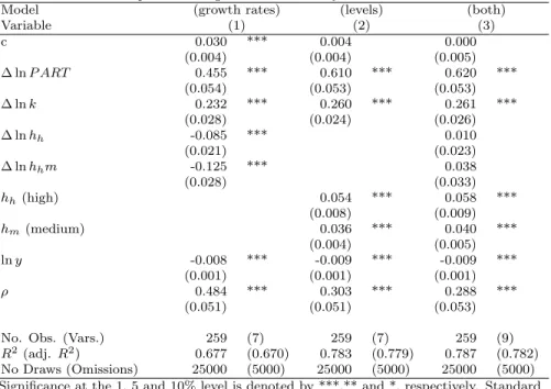
Table 1: Human Capital and Regional Growth - Bayesian SAR Estimation Results

Model (growth rates) (levels) (both)

Variable (1) (2) (3)

c 0.030 *** 0.004 0.000

(0.004) (0.004) (0.005)

∆ lnP ART 0.455 *** 0.610 *** 0.620 ***

(0.054) (0.053) (0.053)

∆ lnk 0.232 *** 0.260 *** 0.261 ***

(0.028) (0.024) (0.026)

∆ lnhh -0.085 *** 0.010

(0.021) (0.023)

∆ lnhhm -0.125 *** 0.038

(0.028) (0.033)

hh(high) 0.054 *** 0.058 ***

(0.008) (0.009)

hm(medium) 0.036 *** 0.040 ***

(0.004) (0.005)

lny -0.008 *** -0.009 *** -0.009 ***

(0.001) (0.001) (0.001)

ρ 0.484 *** 0.303 *** 0.288 ***

(0.051) (0.051) (0.053)

No. Obs. (Vars.) 259 (7) 259 (7) 259 (9)

R² (adj.R²) 0.677 (0.670) 0.783 (0.779) 0.787 (0.782) No Draws (Omissions) 25000 (5000) 25000 (5000) 25000 (5000) Significance at the 1, 5 and 10% level is denoted by ***,** and *, respectively. Standard

errors are in parenthesis.

As we can see from Table 1, model 2 with initial shares of human capital (hh and hm, in column 2) seem to explain more of the variance within the es- timation period than the model with growth rates (in column 1). The growth rates of human capital (in column 1) enter negatively and are highly statistically significant. This may be due to the fact that our estimation period covers more recent years, where the level of human capital of more advanced regions of the Old Member States was nearly saturated and the growth rates have been low.

In the New Member States, regions start with rather low levels of human capital but experience higher growth. Our estimation period might, however, be too short to detect the effects of newly formed human capital. Including both, levels and growth rates, does not substantially improve the fit of the model (measured by R²) and the coefficients on the growth rates are insignificant (see column 3). We, therefore, prefer the model with the levels rather than the growth rates of human capital, because all coefficients are significant and have the expected

sign and size.

Looking at the residuals of the MCMC procedure for the estimated models of Table 1, we found that the heteroscedastic model still hints to several regions as large outliers. After including dummy variables for Romania, the Romanian region ’Bucuresti - Ilfov’, the Greek region ’Sterea Ellada’ and ’Cyprus’, we also tried to include a capital city dummy (like in Capello (2007); Tondl and Vuksic (2007); Cuaresma et al. (2009)), because city regions tend to grow faster than rural regions. For brevity, we do not report all the estimation results for the dummy variables.

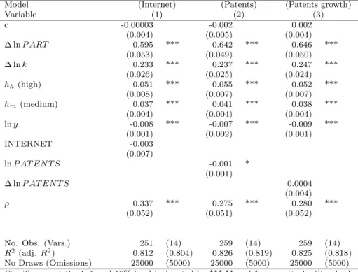
Table 2: Technological Indicators and Growth - Bayesian SAR Estimation Results

Model (Internet) (Patents) (Patents growth)

Variable (1) (2) (3)

c -0.00003 -0.002 0.002

(0.004) (0.005) (0.004)

∆ lnP ART 0.595 *** 0.642 *** 0.646 ***

(0.053) (0.049) (0.050)

∆ lnk 0.233 *** 0.237 *** 0.247 ***

(0.026) (0.025) (0.024)

hh(high) 0.051 *** 0.055 *** 0.052 ***

(0.008) (0.007) (0.007)

hm(medium) 0.037 *** 0.041 *** 0.038 ***

(0.004) (0.004) (0.004)

lny -0.008 *** -0.007 *** -0.009 ***

(0.001) (0.002) (0.001)

INTERNET -0.003

(0.007)

lnP AT EN T S -0.001 *

(0.001)

∆ lnP AT EN T S 0.0004

(0.004)

ρ 0.337 *** 0.275 *** 0.280 ***

(0.052) (0.051) (0.052)

No. Obs. (Vars.) 251 (14) 259 (14) 259 (14)

R²(adj. R²) 0.812 (0.804) 0.826 (0.819) 0.825 (0.818) No Draws (Omissions) 25000 (5000) 25000 (5000) 25000 (5000)

Significance at the 1, 5 and 10% level is denoted by ***,** and *, respectively. Standard errors are in parenthesis.

5.2. Extending the basic model by Patents and Internet access

As a next step, we test the technological and infrastructure variables within our outlier corrected growth regression framework. First, we included the share of Internet users of the year 2001, the log of the patents per million inhabitants (lnP AT EN T S) and the growth rates of patents (∆lnP AT EN T S) as proxies

for the technological output of a region⁶. We see no significant influence of this variable. Column 2 and 3 in Table 2 show the results for the variable patents per million inhabitants. We only find a barely significant, very small and negative coefficient for the logged level variable. This result is not surprising, as this in- dicator describes the innovative output of a region with respect to research and development. As there is no plausible reason to believe that the whole benefit of such an effort should be realized in the same region, we can not expect much of this indicator.

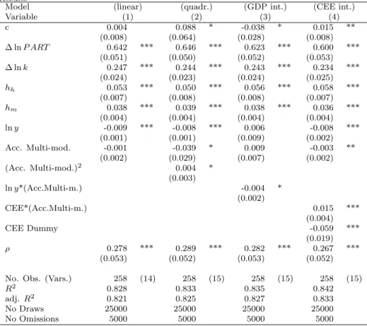
Table 3: Transport Infrastructure (Multimodal-Access) models: Bayesian SAR Estimation Results

Model (linear) (quadr.) (GDP int.) (CEE int.)

Variable (1) (2) (3) (4)

c 0.004 0.088 * -0.038 * 0.015 **

(0.008) (0.064) (0.028) (0.008)

∆ lnP ART 0.642 *** 0.646 *** 0.623 *** 0.600 ***

(0.051) (0.050) (0.052) (0.053)

∆ lnk 0.247 *** 0.244 *** 0.243 *** 0.234 ***

(0.024) (0.023) (0.024) (0.025)

hh 0.053 *** 0.050 *** 0.056 *** 0.058 ***

(0.007) (0.008) (0.008) (0.007)

hm 0.038 *** 0.039 *** 0.038 *** 0.036 ***

(0.004) (0.004) (0.004) (0.004)

lny -0.009 *** -0.008 *** 0.006 -0.008 ***

(0.001) (0.001) (0.009) (0.002)

Acc. Multi-mod. -0.001 -0.039 * 0.009 -0.003 **

(0.002) (0.029) (0.007) (0.002)

(Acc. Multi-mod.)² 0.004 *

(0.003)

lny*(Acc.Multi-m.) -0.004 *

(0.002)

CEE*(Acc.Multi-m.) 0.015 ***

(0.004)

CEE Dummy -0.059 ***

(0.019)

ρ 0.278 *** 0.289 *** 0.282 *** 0.267 ***

(0.053) (0.052) (0.053) (0.052)

No. Obs. (Vars.) 258 (14) 258 (15) 258 (15) 258 (15)

R² 0.828 0.833 0.835 0.842

adj.R² 0.821 0.825 0.827 0.833

No Draws 25000 25000 25000 25000

No Omissions 5000 5000 5000 5000

Significance at the 1, 5 and 10% level is denoted by ***,** and *, respectively. Standard errors are in parenthesis.

6Including the share of Internet users (INTERNET) reduces our sample from 259 regions to 251 as we do not have data in the regions of Denmark, Estonia, Cyprus, Latvia, Lithuania, Luxembourg, Malta and Slovenia.

5.3. Extending the basic model by traffic accessibility

In a further step to include infrastructure into the regional convergence model, we test the ESPON accessibility indicators for their potential to im- prove the growth model. ESPON uses a variable that captures the quality (the potential accessibility as defined by ESPON) rather than the quantity (like road or rail km) of transport infrastructure. The ESPON accessibility indicator is available for road, rail, air, sea and multi-modal and all sub-indicators are highly correlated with each other, resulting in rather similar estimation results when we used them in a extended convergence model. We, therefore, only report the results of the multi-modal accessibility indicator that contain all four modes of transportation. The results are shown in Table 3.

Including just the log of the multi-modal accessibility indicator has no signif- icant effect on growth of GDP per capita⁷. As discussed before, there is reason to believe that the marginal growth enhancing effects of infrastructure might diminish, so we include a quadratic term in the equation (see column 2).

Interestingly, the coefficient of accessibility becomes significant at the 10%

level and remains negative, while the quadratic term is positive and significant.

The reason why we cannot find the expected diminishing marginal returns might be reflected by the choice of the variable. As we have a qualitative indicator of transport infrastructure, the effects seem to turn positive after a certain acces- sibility level is reached. However, the weak significance levels of the indicators is still unsatisfactory. We, therefore, test whether the effects differ with respect to the income level of the region considered. In the columns 3 and 4 of Table 3, we therefore interact the variable with GDP per capita and a Central and Eastern Europe (CEE) dummy variable. Both models suggest that accessibility is mainly a convergence factor for low income regions. This is seen from the negative interaction term (see column 3) and the positive interaction term (see column 4). Also note that the coefficient on the initial GDP per capita turns insignificant (see column 3), and the coefficient of the dummy variable for the CEE countries is negative and significant (see column 4). Thus, taking into account the accessibility of the low income regions explains most of the conver- gence process.

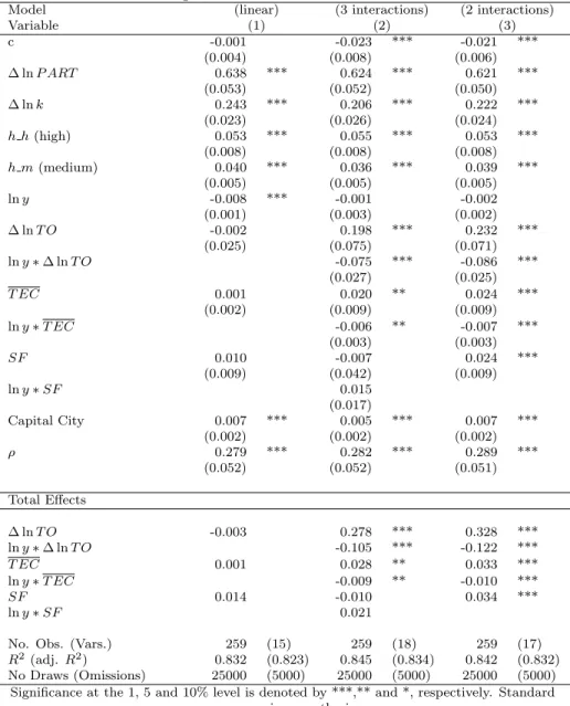
5.4. Linear and Non-Linear Extensions by GLINT Variables

Now we turn to the impact of the variables of interest in this study, the GLINT variables, to see if they can add to the explanation of regional growth in Europe. Prior to the empirical analysis, it is useful to formulate some beliefs about the functional form the GLINT globalization and integration variables that augment the basic convergence growth model. The studies of Badinger

7Note that the sample shrinks to 258 regions, because the ESPON indicator does not report the accessibility of the Canaries Islands.

and Tondl (2005) and Tondl and Vuksic (2007) both used the stock measure of trade flows and FDI stocks respectively, in percent of GDP averaged over the growth period. We are open to the functional form, i.e. in what way to include either the average levels or the growth rates of the GLINT variables into the convergence model. The best results in terms of significance of the coefficients were obtained by including the growth of trade openness (denoted by ∆ lnT O), the average stock of FDI inward stock in percent of GDP (denoted byT EC) and the structural funds expenditures between 2000 and 2006 in percent of average GDP (denoted bySF). Furthermore, we found out that we obtain only signifi- cant results for the GLINT variables when we include them in a non-linear way in the basic convergence model, like in Gonzales-Rivas (2007). The idea is to emphasize the regional convergence process by making the GLINT elasticities level dependent using interaction terms as regressors, and, therefore, we call this extension of the basic model ’Interaction Convergence Model’.

The SAR estimation results of the ’Interactive Convergence Model’ are shown in Table 4. Besides the direct coefficients of the estimation, we also report the total effects – including additionally the spatial feedbacks or indirect effects – calculated according to LeSage and Pace (2009).

The linear convergence model, given in column 1, includes the GLINT glob- alization variables in a spatial regression model (linear means: not interacting with initial GDP per capita). Surprisingly, we see only insignificant coefficients for the three GLINT variables and the coefficients on trade opennessT O have negative signs. Note that the total effects (given at the bottom of Table 4), including the direct effect of the variable and the indirect effect through the spatial autoregressive framework, always exceed the estimates, because we find a positive significant spatial autocorrelation in the sample period. As there is reason to believe that globalization impacts regions differently according to their initial income level (a similar result for the productivity GAP was found in Badinger and Tondl (2005)), we interact the GLINT variables trade, FDI and EU integration with the initial GDP per capita (lny) variable. This speci- fication corresponds to the assumption, that the convergence process within the EU-27 is driven by forces of globalization⁸.

The second column of Table 4 shows the estimates of this ’Interactive Con- vergence Model’. It can be seen that interacting with the initial GDP per capita, the coefficients of trade openness (T O) and FDI inward stock (T EC) in percent of GDP impacted positively on the growth of GDP per capita between 2001 and

8We also tested for the non-linear nature in other variables like the share of Internet users and the number of patents per million inhabitant, both variables that turned out insignificant in the prior analysis. However, we failed to find evidence for non-linearities with respect to initial income per capita, human capital or differing effects for capital city or CEE regions for those variables. Including those non-linearities led to similar results concerning the ranking of winners and losers.

Table 4: Linear and Interaction Convergence Models with GLINT Variables - Bayesian SAR Estimation Results for EU Regions

Model (linear) (3 interactions) (2 interactions)

Variable (1) (2) (3)

c -0.001 -0.023 *** -0.021 ***

(0.004) (0.008) (0.006)

∆ lnP ART 0.638 *** 0.624 *** 0.621 ***

(0.053) (0.052) (0.050)

∆ lnk 0.243 *** 0.206 *** 0.222 ***

(0.023) (0.026) (0.024)

h h(high) 0.053 *** 0.055 *** 0.053 ***

(0.008) (0.008) (0.008)

h m(medium) 0.040 *** 0.036 *** 0.039 ***

(0.005) (0.005) (0.005)

lny -0.008 *** -0.001 -0.002

(0.001) (0.003) (0.002)

∆ lnT O -0.002 0.198 *** 0.232 ***

(0.025) (0.075) (0.071)

lny∗∆ lnT O -0.075 *** -0.086 ***

(0.027) (0.025)

T EC 0.001 0.020 ** 0.024 ***

(0.002) (0.009) (0.009)

lny∗T EC -0.006 ** -0.007 ***

(0.003) (0.003)

SF 0.010 -0.007 0.024 ***

(0.009) (0.042) (0.009)

lny∗SF 0.015

(0.017)

Capital City 0.007 *** 0.005 *** 0.007 ***

(0.002) (0.002) (0.002)

ρ 0.279 *** 0.282 *** 0.289 ***

(0.052) (0.052) (0.051)

Total Effects

∆ lnT O -0.003 0.278 *** 0.328 ***

lny∗∆ lnT O -0.105 *** -0.122 ***

T EC 0.001 0.028 ** 0.033 ***

lny∗T EC -0.009 ** -0.010 ***

SF 0.014 -0.010 0.034 ***

lny∗SF 0.021

No. Obs. (Vars.) 259 (15) 259 (18) 259 (17)

R² (adj.R²) 0.832 (0.823) 0.845 (0.834) 0.842 (0.832) No Draws (Omissions) 25000 (5000) 25000 (5000) 25000 (5000)

Significance at the 1, 5 and 10% level is denoted by ***,** and *, respectively. Standard errors are in parenthesis.

2006. Now, the positive GLINT effects are diminishing with rising initial GDP per capita.

These estimation results favor the hypothesis that globalization through trade and foreign direct investment acts as a (non-linear) convergence factor for less economically developed regions within the EU-27. Moreover, these es- timation results indicate that increasing economic integration explains most of the convergence among those regions, as the coefficient of the unconditional convergence term (lny) decreases substantially in size and turns insignificant.

Both, the coefficients of the structural funds variable (SF) and the interaction term withSF variable are insignificant at conventional confidence levels. Be- cause the (SF) variable is a variable that is aimed at less developed regions in the EU, the inclusion of the interaction term with GDP per capita into the

’Interactive Convergence Model’ is superfluous. Removing the interaction term of the structural funds measures (lny∗SF) yields the results shown in column 3 of Table 4. The coefficient on the integration measure now turns highly sig- nificant and increases by a factor of 2.4 compared to the linear model in column 1. The estimation of this EU integration elasticity means that an increase in structural funds of 1 per cent of regional GDP leads to a growth of 0.024 per cent.

5.5. Interpretation of GLINT Elasticities in the ’Interaction Convergence Model’.

In the ’Interactive Convergence Model’, the elasticities are a linear func- tion of the interaction variable, the log GDP per capita level. The individual elasticities for the 3 GLINT variables are

∂y/∂∆ lnT O = (βT O+βT O,IN T ∗lny)∗∆ lnT O (6)

∂y/∂T EC = β_{T EC,IN T} ∗lny)∗T EC

∂y/∂SF = βSF ∗SF.

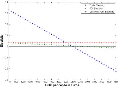
A graphical representation of the level dependent elasticities is given in Fig- ure 1. We see that the coefficients of trade openness (T O) and FDI (T EC) can- not be interpreted as elasticities as in the linear convergence model but depend in the ’Interactive Convergence Model’ on GDP per capita. Figure 1 shows the effect of a 1 percent increase of those measures given a distinct level of income.

For the computation of the elasticities (equation 6) we used the coefficients of column three in Table 4. The estimates of the structural funds expendituresSF imply constant (SF) elasticities (SF²) with respect to GDP per capita⁹. From Figure 1 we see that the trade (∂T O) elasticity and the FDI (∂T EC) elasticity are decreasing functions of lny and change the sign around a GDP per capita

9In models not reported in this paper, we tried different specifications for the structural funds measure. Most interestingly, we found a significant negative quadratic term for the funds, indicating a peak at 30 percent funds in percent of GDP and negative funds effects for 60 percent and over. However, as the sample maximum is 60 percent – for the Greek region

’Voreio Aigaio’, we decided against this

level of approximately 25,000 Euro and 30,000 Euro per capita, respectively.

All regions below this threshold value are potentially benefiting from changes inT O orT EC, while all regions above might not see a direct benefit¹⁰.

Figure 1: GDP per Capita Dependent Elasticities: Contribution of Trade, FDI and Structural Funds

The map in Figure 2 shows the sum of all three globalization measures (GLINT) based on the ’Interaction Convergence Model’ of the lower panel of column three in Table 4. Additionally to the directly estimated coefficients in the model (which includes indirect spatial feedback effects), we sum all the interaction terms with GDP per capita (indexed by INT), so that the total (non-linear) globalization effect on regional growth of all the GLINT variables is calculated by

GLIN T = (β_{T O}+β_{T O,IN T} ∗lny)∗∆ lnT O (7) + (βT EC+βT EC,IN T∗lny)∗T EC

+ βSF ∗SF.

The total GLINT effects in Figure 2 are given in percentage points, and we have clustered the regions into 3 groups: the globalization winners (in green) with a growth bonus between 0.5 and 4 percentage points, the globalization

10Note that a possible evaluation target of regional EU politics could be a elasticity curve of GLINT variables that has negative slope but is rather flat and close to zero for rich regions.

losers (in red) with a negative impact of 0.5 or more percentage points and re- gions that were basically unaffected by globalization forces through the GLINT variables during the estimation period (no color). The number next to the leg- end shows the number of regions (from a total of 259) falling into these 3 groups.

We see that almost two thirds of the regions have not been strongly affected by the GLINT globalization forces between 2001 and 2006. The winners are the New Member States of the EU, Greece, Portugal, Western Spain, North- ern Ireland and Southern Italy. Clearly, as the interaction convergence model implies, these regions are found all on the lower end of GDP per capita scale in 2001. According to these 3 classes, only 14 regions can be identified as net losers of globalization, because they started already at a high initial GDP per capita level, and these are mostly German, Dutch, Belgian and Austrian re- gions¹¹. Note that these regions are large cities like Vienna, Munich, Frankfurt, Brussels, Amsterdam, Stockholm and Helsinki. Those cities might not really be losers at the end of the day, since some of them enjoy the capital bonus (dummy variable: ’Capital City’) of about 0.7 percentage points of growth in our model might overcome these distributional losses (via GLINT) by other aggregation forces that we could not quantify and have not yet taken care off.

Figure 3 displays the boxplot distribution of the net impacts of the glob- alization indicators according to the MCMC draws of the coefficients. This is the (posterior) estimated contribution of the GLINT variables in the interac- tion convergence model. The distribution is obtained by inserting the MCMC sample into the definition of the sum of the GLINT contribution in (7). The distribution of the total GLINT effects have been ordered and gives answers to 2 questions: Which regions have significant positive (negative) GLINT contri- butions and which regions are the most volatile regions with respect to GLINT contributions. For the first question we rank the regions according to the median of the (posterior) GLINT contributions and for the second question we rank the regions according to the interquartile range (IQR) to rule out any effects due to outliers in the sampling distribution. We see that there are more GLINT distri- butions that lie on the positive side than on the negative side. That means that looking at the total GLINT effects there are more regions that are winners than losers. But the majority of regions might experience either positive or negative effects of the 3 GLINT contributions. If it comes to the volatility of these total GLINT influences, we see no clear correlation with the median GLINT effects.

It seems that volatility across regions follows different influences and this effect needs more attention for future regional growth modeling. Different modeling strategies might have to be taken into account to find out if the volatile re- sponses of regions to globalization influences can be explained.

11Luxembourg, Bruxelles, Prov. Antwerpen, Prov. Brabant Wallon, Stuttgart, Karl- sruhe, Oberbayern, Bremen, Hamburg, Darmstadt, Groningen, Utrecht, Noord-Holland, Zuid- Holland, Wien, Salzburg, Vorarlberg, Etel¨a-Suomi, Stockholm and Inner London.

Figure 2: Net Impacts of Globalization (GLINT) Variables on GDP per Capita Growth, 2001-2006

Figure 3: MCMC Distribution of GLINT Effects (GLIN T) on GDP per Capita Growth, 2001-2006

Figure 4: GLINT Scattergram: A Cone formed by Median vs. Interquartile Range (IQR) of the GLINT Effects Distribution

Figure 4 can be seen as a risk analysis of the total GLINT contributions.

Points colored in red (green) indicate the GLINT losers (winners) of figure 2.

Most of the growth rates and the volatility of the GLINT contributions are small and concentrate around the zero vortex and forms a triangular cone. But some growth rates can become large and are associated with larger dispersions from the growth rate distribution. The positive branch is larger than the negative branch, both in terms of the size of the mean and the IQR. This can be seen as good news, since more regions will benefit and the size of the effects are larger for the regions in the positive branch. The fact that many regions cluster around the vortex is not too surprising, since GLINT effects are not expected to be the largest effects in a regional growth model, that is exposed to many heterogeneous influences.

5.6. Sensitivity analysis

To check the sensitivity of the estimation results of the interaction conver- gence model, we performed three sensitivity checks, which are shown in Table 5. The estimates in column 1 were estimated using the feasible generalized spa- tial two-stage least squares (2SLS) estimator proposed by Kelejian and Prucha (1998) with a contiguity matrix for the spatial error component (with parameter λ). We see that the implications of the interaction convergence model do not change, though the interaction terms and the structural funds measure are esti- mated less precisely. Next, we include a Central and Eastern European (CEE) dummy, to check whether our results are driven by a growth bonus of the New Member States. The coefficient of theCEE dummy is positive and significant at a ten percent level. Nevertheless, all GLINT globalization measures have significantly estimated coefficient, with the coefficient of trade openness being slightly smaller.

The third column (CEE interactions) shows the results when different fac- tor elasticities for Old and New Member States are considered. We extend the GDP interaction model with another 4 interaction variables, but now we also interact the CEE dummy with the 4 factor variableshh, hm, ∆ lnP ART and

∆ lnk. Except for the elasticity of tertiary human capital (hh) and an only marginally significant difference for the participation rate, there do not seem to be significant differences in the factor shares and the explanatory power of the

’double interaction model’. However, the coefficient of our measure of techno- logical globalization – the FDI inward stock per capita – decreases to about half the size and is now insignificant. This might be an indication that the higher elasticity of tertiary human capital in the CEE countries is connected to the FDI proxy variable and thus to the technology transfer effect after the fall of the iron curtain.

Finally, an additional model including interactions of the FDI measure with the educational variables, shows significant interactions of FDI with higher ed- ucation (hh). The results for this model are not reported here, as the coefficient