Guido B 1
Joan D 1
Michaël P 2
Gilles V A 1
http://keccak.noekeon.org/
Version3.0 January 14, 2011
1STMicroelectronics
2NXP Semiconductors
1 K specifications 7
1.1 Conventions and notation . . . 7
1.1.1 Bitstrings . . . 7
1.1.2 Padding rules . . . 7
1.2 The K -f permutations . . . 7
1.3 The sponge construction . . . 8
1.4 The K sponge functions . . . 9
1.5 Security claim for the K sponge functions . . . 9
1.6 Parts of the state . . . 10
2 TheK -f permutations 13 2.1 Translation invariance . . . 13
2.2 The Matryoshka structure . . . 14
2.3 The step mappings of K -f . . . 14
2.3.1 Properties ofχ . . . 15
2.3.2 Properties ofθ . . . 17
2.3.3 Properties ofπ . . . 19
2.3.4 Properties ofρ . . . 21
2.3.5 Properties ofι . . . 22
2.3.6 The order of steps within a round . . . 23
2.4 Differential and linear cryptanalysis . . . 23
2.4.1 A formalism for describing trails adapted to K -f . . . 23
2.4.2 The Matryoshka consequence . . . 24
2.4.3 The column parity kernel . . . 25
2.4.4 One and two-round trails . . . 25
2.4.5 Three-round trails: kernel vortices . . . 26
2.4.6 Beyond three-round trails: choice ofπ . . . 27
2.4.7 Truncated trails and differentials . . . 29
2.4.8 Other group operations . . . 29
2.4.9 Differential and linear cryptanalysis variants . . . 29
2.5 Solving constrained-input constrained-output (CICO) problems . . . 30
2.6 Strength in keyed mode . . . 30
2.7 Symmetry weaknesses . . . 31
3 Trail propagation inK -f 33 3.1 Relations between different kinds of weight . . . 33
3.2 Propagation properties related to the linear stepθ . . . 35
3.3 Exhaustive trail search . . . 36
3.3.1 Upper bound for the weight of two-round trails to scan . . . 36
3.4.1 Construction of tame trails . . . 41
3.4.2 Bounds for three-round tame trails . . . 42
3.4.3 Bounds for four-round tame trails . . . 44
4 Analysis ofK -f 45 4.1 Algebraic normal form . . . 45
4.1.1 Statistical tests . . . 45
4.1.2 Symmetric trails . . . 46
4.1.3 Slide a acks . . . 48
4.2 Solving CICO problems algebraically . . . 48
4.2.1 The goal . . . 48
4.2.2 The supporting so ware . . . 48
4.2.3 The experiments . . . 49
4.2.4 Third-party analysis . . . 51
4.3 Properties of K -f[25] . . . 51
4.3.1 Algebraic normal statistics . . . 51
4.3.2 Differential probability distributions . . . 52
4.3.3 Correlation distributions . . . 53
4.3.4 Cycle distributions . . . 57
4.4 Distinguishers exploiting low algebraic degree . . . 59
4.4.1 Zero-sum distinguishers . . . 60
4.4.2 Pre-image a acks . . . 62
5 Design rationale summary 63 5.1 Choosing the sponge construction . . . 63
5.2 Choosing an iterated permutation . . . 64
5.3 Designing the K -f permutations . . . 64
5.4 Strength estimation . . . 65
In this document we specify, analyze and motivate the design of the cryptographic primitive K . Based on the sponge construction, K inherits many of its features. We gath- ered all our analysis on sponge functions in a separate document titledCryptographic sponge functions[8]. Reading it is a requisite for understanding the usability and security properties of K and the security requirements for K -f, the permutation used in K .
Other documents and files are of interest to the readers of this K reference.
• This document comes with a set of files containing results of tests and experiments, available fromhttp://keccak.noekeon.org/.
• The implementation aspects are covered in a separate document K implementation overview, which treats so ware and hardware techniques and results, with or without protection against side-channel a acks [10].
• Also, K T , an open-source so ware aimed at helping analyze K [9].
This document is organized as follows. Chapter 1 contains the formal specifications of K . The subsequent three chapters are dedicated to the K -f permutations:
• Chapter 2 explains the properties of the building blocks of K -f and motivates the choices made in its design.
• Chapter 3 is dedicated to trail propagation in K -f.
• Chapter 4 covers all other analysis of K -f.
Finally, Chapter 5 summarizes the design choices behind K and contains our estimation of the safety margin of K .
Acknowledgments
We wish to thank (in no particular order) Charles Bouillaguet and Pierre-Alain Fouque for discussing their results later published in [13] with us, Dmitry Khovratovich for discussing with us the results published in [29] and for his analysis in [1], Jean-Philippe Aumasson for his analysis in [1] and [2], Joel Lathrop for his analysis in [34] and Willi Meier for his analysis in [2], Anne Canteaut and Christina Boura for their analysis in [15, 14, 16], Christophe De Cannière for his analysis in [16], Paweł Morawiecki and Marian Srebrny for their analysis in [36], Dan Bernstein for his analysis in [3], Ming Duan and Xuejia Lai for their analysis in [26], Yves Moulart, Bernard Kasser and all our colleagues at STMicroelectronics and NXP Semiconductors for creating the working environment in which we could work on this. Fi- nally we would like to thankAgentschap voor Innovatie door Wetenschap en Technologie(IWT) for funding two of the authors (Joan Daemen and Gilles Van Assche).
K specifications
K (pronounced [kɛtʃak]) is a family of sponge functions [8] that use as a building block a permutation from a set of 7 permutations. In this chapter, we introduce our conventions and notation, specify the 7 permutations underlying K and the K sponge functions.
We also give conventions for naming parts of the K state.
1.1 Conventions and notation
We denote the absolute value of a real numberxis denoted by|x|. 1.1.1 Bitstrings
We denote the length in bits of a bitstringM by|M|. A bitstring Mcan be considered as a sequence of blocks of some fixed lengthx, where the last block may be shorter. The number of blocks ofMis denoted by|M|x. The blocks ofMare denoted byMiand the index ranges from0to|M|x−1.
We denote the set of all bitstrings including the empty string by Z∗2 and excluding the empty string byZ+2. The set of infinite-length bitstrings is denoted byZ2∞.
1.1.2 Padding rules
For the padding rule we use the following notation: the padding of a message M to a se- quence ofx-bit blocks is denoted by M||pad[x](|M|). This notation highlights that we only consider padding rules that append a bitstring that is fully determined by the bitlength ofM and the block lengthx. We may omit[x],(|M|)or both if their value is clear from the context.
K makes use of themulti-ratepadding.
Definition 1. Multi-rate padding, denoted bypad10∗1, appends a single bit 1 followed by the minimum number of bits 0 followed by a single bit 1 such that the length of the result is a multiple of the block length.
Multi-rate padding appends at least 2 bits and at most the number of bits in a block plus one.
1.2 The K - f permutations
There are 7 K -f permutations, indicated by K -f[b], where b = 25×2ℓ and ℓ ranges from 0 to 6. K -f[b]is a permutation overZb2, where the bits ofsare numbered
follows that indexing starts from zero. The mapping between the bits ofsand those ofais s[w(5y+x) +z] =a[x][y][z]. Expressions in thexandycoordinates should be taken modulo 5 and expressions in thezcoordinate modulow. We may sometimes omit the[z]index, both the[y][z]indices or all three indices, implying that the statement is valid for all values of the omi ed indices.
K -f[b]is an iterated permutation, consisting of a sequence ofnrroundsR, indexed withirfrom 0 tonr−1. A round consists of five steps:
R=ι◦χ◦π◦ρ◦θ, with
θ : a[x][y][z] ←a[x][y][z] +
∑
4 y′=0a[x−1][y′][z] +
∑
4 y′=0a[x+1][y′][z−1], ρ: a[x][y][z] ←a[x][y][z−(t+1)(t+2)/2],
withtsatisfying0≤ t<24and (0 1
2 3 )t(
1 0
)
= (x
y )
inGF(5)2×2, ort=−1ifx=y=0,
π: a[x][y] ←a[x′][y′], with (x
y )
= (0 1
2 3 ) (x′
y′ )
, χ: a[x] ←a[x] + (a[x+1] +1)a[x+2],
ι: a ←a+RC[ir].
The additions and multiplications between the terms are inGF(2). With the exception of the value of the round constantsRC[ir], these rounds are identical. The round constants are given by (with the first index denoting the round number)
RC[ir][0][0][2j−1] =rc[j+7ir]for all0≤ j≤ℓ,
and all other values ofRC[ir][x][y][z]are zero. The valuesrc[t] ∈ GF(2)are defined as the output of a binary linear feedback shi register (LFSR):
rc[t] = (
xtmodx8+x6+x5+x4+1 )
modxinGF(2)[x].
The number of roundsnris determined by the width of the permutation, namely, nr =12+2ℓ.
1.3 The sponge construction
The sponge construction [8] builds a function [f, pad,r]with variable-length input and arbitrary output length using a fixed-length permutation (or transformation)f, a padding rule “pad” and a parameterbitrater. The permutation f operates on a fixed number of bits, thewidthb. The valuec=b−ris called thecapacity.
For the padding rule we use the following notation: the padding of a message M to a sequence ofx-bit blocks is denoted byM||pad[x](|M|), where|M|is the length ofMin bits.
Initially, the state has value0b, called theroot state. The root state has a fixed value and shall never be considered as an input. This is crucial for the security of the sponge construc- tion.
Algorithm 1The sponge construction [f, pad,r] Require: r<b
Interface: Z=sponge(M,ℓ)withM∈Z∗2, integerℓ >0andZ∈Zℓ2 P= M||pad[r](|M|)
s=0b
fori=0to|P|r−1do s= s⊕(Pi||0b−r) s= f(s)
end for Z= ⌊s⌋r
while|Z|rr < ℓdo s= f(s)
Z= Z||⌊s⌋r
end while return ⌊Z⌋ℓ
1.4 The K sponge functions
We define the sponge function denoted by K [r,c]by applying the sponge construction as specified in Algorithm 1 with K -f[r+c], multi-rate padding and the bitrater.
K [r,c], [K -f[r+c], pad10∗1,r].
This specifies K [r,c] for any combination of r > 0 and c such that r+c is a width supported by the K -f permutations.
The default value forris1600−cand the default value forcis 576:
K [c],K [r =1600−c,c], K [],K [c=576].
1.5 Security claim for the K sponge functions
For each of the supported parameter values, we make aflat sponge claim[8, Section “The flat sponge claim”].
Claim 1. The expected success probability of any a ack againstK [r,c]with a workload equiv- alent toNcalls toK -f[r+c]or its inverse shall be smaller than or equal to that for a random oracle plus
1−exp
(−N(N+1)2−(c+1) )
.
We exclude hereweaknessesdue to the mere fact that K -f[r+c]can be described com- pactly and can be efficiently executed, e.g., the so-called random oracle implementation impossibility [8, Section “The impossibility of implementing a random oracle”].
Note that the claimed capacity is equal to the capacity used by the sponge construction.
properties of K -f.
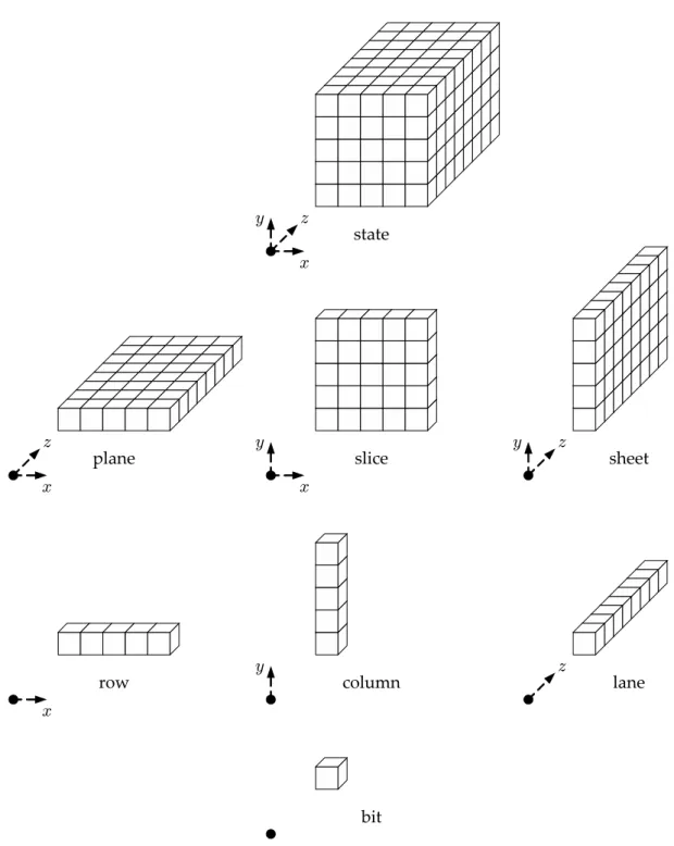
The one-dimensional parts are:
• Arowis a set of 5 bits with constantyandzcoordinates.
• Acolumnis a set of 5 bits with constantxandzcoordinates.
• Alaneis a set ofwbits with constantxandycoordinates.
The two-dimensional parts are:
• Asheetis a set of5wbits with constantxcoordinate.
• Aplaneis a set of5wbits with constantycoordinate.
• Asliceis a set of25bits with constantzcoordinate.
Figure 1.1: Naming conventions for parts of the K -f state
The K - f permutations
This chapter discusses the properties of the K -f permutations that are relevant for the security of K . A er discussing some structural properties, we treat the different map- pings that make up the round function. This is followed by a discussion of differential and linear cryptanalysis to motivate certain design choices. Subsequently, we briefly discuss the applicability of a number of cryptanalytic techniques to K -f.
2.1 Translation invariance
Let b = τ(a) with τ a mapping that translates the state by 1 bit in the direction of the z axis. For0 < z < wwe haveb[x][y][z] = a[x][y][z−1]and forz = 0we have b[x][y][0] = a[x][y][w−1]. Translating overt bits givesb[x][y][z] = a[x][y][(z−t)modw]. In general, a translationτ[tx][ty][tz]can be characterized by a vector with three components(tx,ty,tz) and this gives:
b[x][y][z] = a[(x−tx)mod 5][(y−ty)mod 5][(z−tz)mod w]. Now we can definetranslation-invariance.
Definition 2. A mappingαistranslation-invariantin direction(tx,ty,tz)if τ[tx][ty][tz]◦α= α◦τ[tx][ty][tz].
Let us now define thez-period of a state.
Definition 3. Thez-period of a stateais the smallest integerd>0such that:
∀x,y∈Z5and∀z ∈Zw :a[x][y][(z+d)modw] =a[x][y][z].
first slicesa[.][.][z]withz<d. We call this thez-reduced representationofa.
• For a givenw, thez-period defines a partition on the states.
• The number of states withz-perioddis zero ifddoes not dividewand fully determined bydonly, otherwise.
• Forwvalues that are a power of two (the only ones allowed in K ), the state space consists of the states withz-period 1, 2,22up to2ℓ =w.
• The number of states withz-period 1 is225. The number of states withz-period2d for d ≥1is22d25−22d−125.
• There is a one-to-one mapping between the statesa′withz-perioddfor any lane length wthat is a multiple ofdand the statesawith z-periodd of lane lengthd: a′[.][.][z] = a[.][.][zmodd].
• Ifαis translation-invariant in the direction of thez axis, the z-period ofα(a)divides thez-period ofa. Moreover, thez-reduced state ofα(a)is independent ofw.
• Ifαis injective and translation-invariant in the direction of thezaxis,αpreserves the z-period.
2.2 The Matryoshka structure
With the exception of ι, all step mappings of the K -f round function are translation- invariant in the direction of thezaxis. This allows the introduction of a size parameter that can easily be varied without having to re-specify the step mappings. As in several types of analysis abstraction can be made of the addition of constants, this allows the re-use of structures for small width versions as symmetric structures for large width versions. We refer to Section 2.4.2 for an example. As the allowed lane lengths are all powers of two, every smaller lane length divides a larger lane length. So, as the propagation structures for smaller width version are embedded as symmetric structure in larger width versions, we call it Matryoshka, a er the well-known Russian dolls.
2.3 The step mappings of K - f
A round is composed from a sequence of dedicated mappings, each one with its particular task. The steps have a simple description leading to a specification that is compact and in which no trapdoor can be hidden.
Mapping thelanesof the state, i.e., the one-dimensional sub-arrays in the direction of the zaxis, onto CPU words, results in simple and efficient so ware implementation for the step mappings. We start the discussion of each of the step mappings by pseudocode where the variablesa[x,y]represent the old values of lanes andA[x,y]the new values. The operations on the lanes are limited to bitwise Boolean operations and rotations. In our pseudocode we denote byROT(a,d)a translation ofaoverdbits where bit in positionzis mapped to position z+dmodw. If the CPU word length equals the lane length, the la er can be implemented
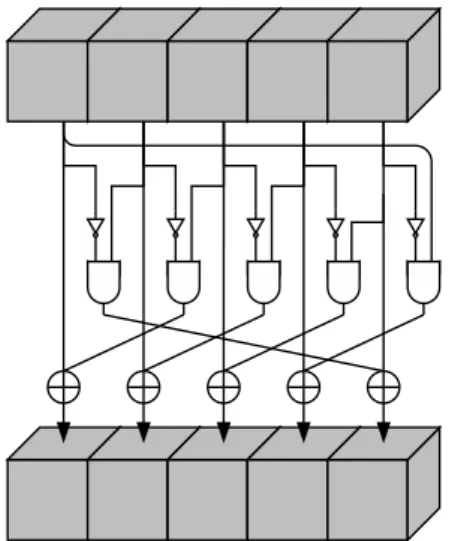
Figure 2.1: χapplied to a single row
with rotate instructions. Otherwise a number of shi and bitwise Boolean instructions must be combined or bit-interleaving can be applied [10].
In this section we discuss the difference propagation and input-output correlation prop- erties of the different mappings. We refer to [8, Sections “Differential cryptanalysis” and
“Linear cryptanalysis”] for an introduction of the terminology and concepts.
2.3.1 Properties ofχ
Figure 2.1 contains a schematic representation ofχand Algorithm 2 its pseudocode.
Algorithm 2χ fory=0to 4do
forx =0to 4do
A[x,y] =a[x,y]⊕((NOTa[x+1,y])ANDa[x+2,y]) end for
end for
χis the only nonlinear mapping in K -f. Without it, the K -f round function would be linear. It can be seen as the parallel application of5w S-boxes operating on 5- bit rows. χis translation-invariant in all directions and has algebraic degree two. This has consequences for its differential propagation and correlation properties. We discuss these in short in Sections 2.3.1.1 and Section 2.3.1.2 and refer to [20, Section 6.9] for an in-depth treatment of these aspects.
χis invertible but its inverse is of a different nature thanχitself. For example, it does not have algebraic degree 2. We refer to [20, Section 6.6.2] for an algorithm for computing the inverse ofχ.
χis simply the complement of the nonlinear function calledγ, that is used in R G [4], P [21] and several other ciphers [20]. We have chosen it for its simple nonlinear propagation properties, its simple algebraic expression and its low gate count: one XOR, one AND and one NOT operation per state bit.
corresponding (restriction) weightwr(a′,b′) =wr(a′)is an integer that only depends on the input difference a′. A possible differential imposeswr(a′)linear conditions on the bits of inputa.
We now provide a recipe for constructing the affine variety of output differences corre- sponding to an input difference, applied to a single row. Indices shall be taken modulo 5 (or in general, the length of the register). We denote byδ(i)a pa ern with a single nonzero bit in positioniandδ(i,j)a pa ern with only non-zero bits in positionsiandj.
We can characterize the linear affine variety of the possible output differences by an offset A′ and a basis⟨cj⟩. The offset isA′ =χ(a′). We construct the basis⟨cj⟩by adding vectors to it while running over the bit positionsi:
• Ifa′ia′i+1a′i+2a′i+3∈ {·100,·11·, 001·}, extend the basis withδ(i).
• Ifa′ia′i+1a′i+2a′i+3=·101, extend the basis withδ(i,i+1).
This algorithm is implemented in K T [9]. The (restriction) weight of a difference is equal to its Hamming weight plus the number of pa erns 001. The all-1 input difference results in the affine variety of odd-parity pa erns and has weight 4 (or in general the length of the register minus 1). Among the 31 non-zero differences, 5 have weight 2, 15 weight 3 and 11 weight 4.
A differential(a′,b′)leads to a number of conditions on the bits of the absolute valuea.
LetB= A′⊕b′ = χ(a′)⊕b′, then we can construct the conditions onaby running over each bit positioni:
• a′i+1ai′+2=10imposes the conditionai+2 =Bi.
• a′i+1ai′+2=11imposes the conditionai+1⊕ai+2 =Bi .
• a′i+1ai′+2=01imposes the conditionai+1 =Bi.
The generation of these conditions given a differential trail is implemented in K T [9].
2.3.1.2 Correlation properties
Thanks to the fact that χ has algebraic degree 2, for a given output mask u, the space of input mask v whose parities have a non-zero correlation with the parity determined byu form a linear affine variety. This variety has2wc(v,u) elements, withwc(v,u) = wc(u) the (correlation) weight function, which is an even integer that only depends on the output mask u. Moreover, the magnitude of a correlation overχis either zero or equal to2−wc(u)/2.
We now provide a recipe for constructing the affine variety of input masks corresponding to an output mask, applied to a single row. Indices shall again be taken modulo 5 (or in general, the length of the register). We use the term1-run of lengthℓto denote a sequence of ℓ1-bits preceded and followed by a 0-bit.
We characterize the linear affine variety with an offsetU′ and a basis⟨cj⟩and build the offset and basis by running over the output mask. First initialize the offset to 0 and the basis to the empty set. Then for each of the 1-runsasas+1. . .as+ℓ−1do the following:
• Add a 1 in positionsof the offsetU′.
• Seti=s, the starting position of the 1-run.
• As long asaiai+1 = 11extend the basis withδ(i+1,i+3)andδ(i+2), add 2 toiand continue.
• Ifaiai+1 =10extend the basis withδ(i+1)andδ(i+2).
This algorithm is implemented in K T [9]. The (correlation) weight of a mask is equal to its Hamming weight plus the number of 1-runs of odd length. The all-1 output mask results in the affine variety of odd-parity pa erns and has weight 4 (or in general the length of the register minus 1). Of the 31 non-zero mask, 10 have weight 2 and 21 have weight 4.
2.3.2 Properties ofθ
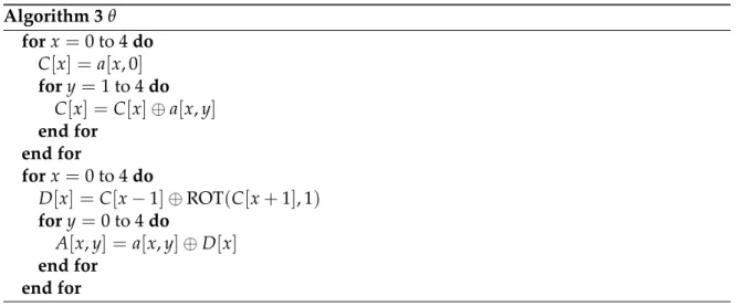
Figure 2.2 contains a schematic representation ofθand Algorithm 3 its pseudocode.
Algorithm 3θ forx =0to 4do
C[x] =a[x, 0] fory=1to 4do
C[x] =C[x]⊕a[x,y] end for
end for
forx =0to 4do
D[x] =C[x−1]⊕ROT(C[x+1], 1) fory=0to 4do
A[x,y] =a[x,y]⊕D[x] end for
end for
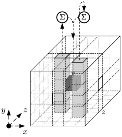
Theθ mapping is linear and aimed at diffusion and is translation-invariant in all direc- tions. Its effect can be described as follows: it adds to each bita[x][y][z]the bitwise sum of the parities of two columns: that ofa[x−1][·][z]and that ofa[x+1][·][z−1]. Withoutθ, the K -f round function would not provide diffusion of any significance. Theθ mapping has a branch number as low as 4 but provides a high level of diffusion on the average. We refer to Section 2.4.3 for a more detailed treatment of this.
In fact, we have chosenθ for its high average diffusion and low gate count: two XORs per bit. Thanks to the interaction withχeach bit at the input of a round potentially affects 31 bits at its output and each bit at the output of a round depends on 31 bits at its input. Note that without the translation of one of the two sheet parities this would only be 25 bits.
2.3.2.1 The inverse mapping
Computing the inverse ofθcan be done by adopting a polynomial notation. The state can be represented by a polynomial in the three variables x,y and z with binary coefficients.
x
y z z
Figure 2.2:θ applied to a single bit
Here the coefficient of the monomialxiyjzk denotes the value of bita[i][j][k]. The exponents i and j range from 0 to 4 and the exponentk ranges from0 to w−1. In this representa- tion a translationτ[tx][ty][tz]corresponds with the multiplication by the monomialxtxytyztz modulo the three polynomials1+x5,1+y5and1+zw. More exactly, the polynomial rep- resenting the state is an element of a polynomial quotient ring defined by the polynomial ring overGF(2)[x,y,z]modulo the ideal generated by⟨
1+x5, 1+y5, 1+zw⟩. A translation corresponds with multiplication byxtxytyztz in this quotient ring. The z-period of a state a isdifdis the smallest nonzero integer such that1+zd dividesa. Let a′ be the polynomial corresponding to thez-reduced state ofa, thenacan be wri en as
a = (1+zd+z2d+. . .+zw−d)×a′ = 1+zw 1+zd ×a′ .
When the state is represented by a polynomial, the mappingθ can be expressed as the multiplication (in the quotient ring defined above) by the following polynomial :
1+y¯ (
x+x4z )
withy¯=
∑
4 i=0yi = 1+y5
1+y . (2.1)
The inverse ofθcorresponds with the multiplication by the polynomial that is the inverse of polynomial (2.1). Forw= 64, we have computed this with the open source mathematics so ware SAGE [38] a er doing a number of manipulations. First, we assume it is of the form 1+yQ¯ withQa polynomial inxandzonly:
(
1+y¯(x+x4z)
)×(1+yQ¯ ) =1 mod
⟨
1+x5, 1+y5, 1+z64
⟩ .
Working this out and usingy¯2 =y¯yields
Q=1+ (1+x+x4z)−1mod
⟨
1+x5, 1+z64
⟩ .
The inverse of1+x+x4zcan be computed with a variant of the extended Euclidian algo- rithm for polynomials in multiple variables. At the time of writing this was unfortunately
not supported by SAGE. Therefore, we reduced the number of variables to one by using the change of variablest= x−2z. We havex =t192andx4z=t193, yielding:
Q=1+ (1+t192+t193)−1mod(1+t320).
By performing a change in variables fromttoxandzagain,Qis obtained.
Forw < 64, the inverse can simply be found by reducingQmodulo1+zw. Forw= 1, the inverse ofθreduces to1+y¯(x2+x3).
For all values ofw=2ℓ, the Hamming weight of the polynomial ofθ−1is of the orderb/2.
This implies that applyingθ−1to a difference with a single active bit results in a difference with about half of the bits active. Similarly, a mask at the output ofθ−1 determines a mask at its input with about half of the bits active.
2.3.2.2 Propagation of linear masks
A linear Boolean function defined by a maskuat the output of a linear function has non-zero correlation to a single linear Boolean function at its input. Given the matrix representation of the linear function, it is easy to express the relation between the input and output mask.
Givenb= Ma, we have:
uTb=uTMa= (MTu)Ta.
It follow thatuTbis correlated tovTawithv = MTuwith correlation 1. We say that a mask uat the output of a linear mapping M propagates tov = MTu at its input. We denote the mapping defined byMT thetransposeof M.
Asθis linear, we havev =θT(u), withua mask at the output ofθ,va mask at its input and whereθTthe transpose ofθ. We now determine the expression for the transpose ofθin the formalism of [5]. Letb=θ(a)and
x,y,z
∑
u[x][y][z]b[x][y][z] =
∑
x,y,z
v[x][y][z]a[x][y][z].
Filling in the value ofb[x][y][z]from the specification ofθin [5] and working this out yields:
x,y,z
∑
u[x][y][z]b[x][y][z] =
x,y,z
∑
(
u[x][y][z] +
∑
y′
u[x+1][y′][z] +
∑
y′
u[x−1][y′][z+1] )
a[x][y][z]
It follows that:
v=θT(u)⇔v[x][y][z] =u[x][y][z] +
∑
y′
u[x+1][y′][z] +
∑
y′
u[x−1][y′][z+1] (2.2)
In polynomial notation the application ofθTis a multiplication by 1+y¯
(
x4+xz4 )
.
2.3.3 Properties ofπ
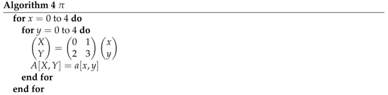
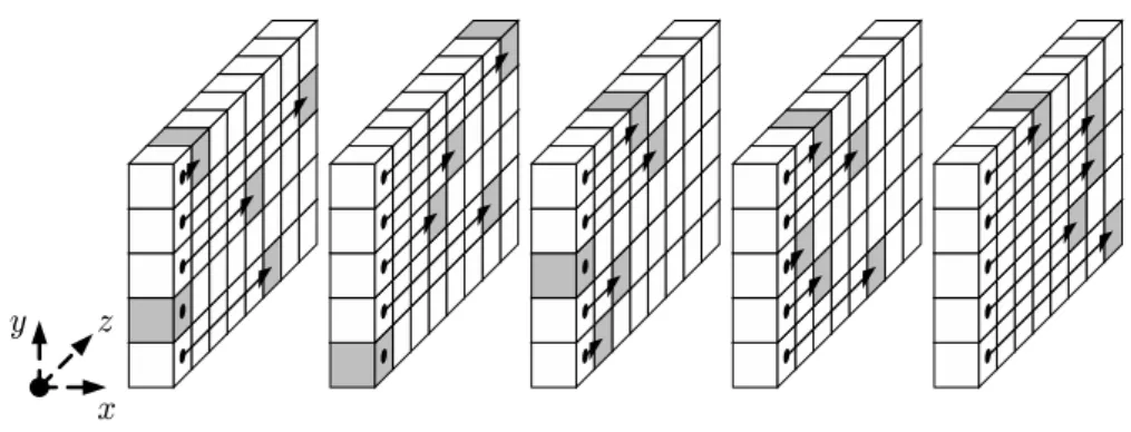
Figure 2.3 contains a schematic representation ofπand Algorithm 4 its pseudocode.
Note that in an efficient programπcan be implemented implicitly by addressing.
Algorithm 4π forx=0to 4do
for(y=0to 4do X
Y )
= (0 1
2 3 ) (x
y )
A[X,Y] =a[x,y] end for
end for
Figure 2.3:πapplied to a slice. Note thatx=y=0is depicted at the center of the slice.
The mapping π is a transposition of the lanes that provides dispersion aimed at long- term diffusion. Without it, K -f would exhibit periodic trails of low weight. πoperates in a linear way on the coordinates(x,y): the lane in position(x,y)goes to position(x,y)MT, withM=(0 12 3)a 2 by 2 matrix with elements inGF(5). It follows that the lane in the origin (0, 0)does not change position. Asπoperates on the slices independently, it is translation- invariant in thez-direction. The inverse ofπis defined byM−1.
Within a slice, we can define 6 axes, where each axis defines adirectionthat partitions the 25 positions of a slice in 5 sets:
• xaxis: rows or planes;
• yaxis: columns or sheets;
• y=xaxis: rising 1-slope;
• y=−xaxis: falling 1-slope;
• y=2xaxis: rising 2-slope;
• y=−2xaxis: falling 2-slope;
Thexaxis is just the row through the origin, theyaxis is the column through the origin, etc.
There are many matrices that could be used forπ. In fact, the invertible 2 by 2 matrices with elements inGF(5)with the matrix multiplication form a group with 480 elements con- taining elements of order 1, 2, 3, 4, 5, 6, 8, 10, 12, 20 and 24. Each of these matrices defines a permutation on the 6 axes, and equivalently, on the 6 directions. Thanks to its linearity, the 5 positions on an axis are mapped to 5 positions on an axis (not necessarily the same).
Similarly, the 5 positions that are on a line parallel to an axis, are mapped to 5 positions on a line parallel to an axis.
Forπwe have chosen a matrix that defines a permutation of the axes where they are in a single cycle of length 6 for reasons explained in Section 2.4.6. Implementingπin hardware requires no gates but results in wiring.
Asπis a linear function, a masku at the output propagates to the maskvat the input withv= πT(u)(see Section 2.3.2.2). Moreover, we haveπT =π−1, yieldingu=π(v). This follows directly from the fact thatπis a bit transposition and that subsequently its matrix is orthogonal: MTM = I.
2.3.4 Properties ofρ
Figure 2.4 contains a schematic representation ofρ, while Table 2.1 lists its translation offsets.
Algorithm 5 gives pseudocode forρ.
Algorithm 5ρ A[0, 0] = a[0, 0] (x
y )
= (1
0 ) fort=0to 23do
A[x,y] =ROT(a[x,y],(t+1)(t+2)/2) (x
y )
= (0 1
2 3 ) (x
y ) end for
Figure 2.4:ρapplied to the lanes. Note thatx=y=0is depicted at the center of the slices.
x =3 x=4 x=0 x=1 x=2
y=2 153 231 3 10 171
y=1 55 276 36 300 6
y=0 28 91 0 1 190
y=4 120 78 210 66 253
y=3 21 136 105 45 15
Table 2.1: The offsets ofρ
The mappingρ consists of translations within the lanes aimed at providing inter-slice dispersion. Without it, diffusion between the slices would be very slow. It is translation- invariant in thez-direction. The inverse ofρis the set of lane translations where the constants are the same but the direction is reversed.
The 25 translation constants are the values defined byi(i+1)/2modulo the lane length.
It can be proven that for anyℓ, the sequencei(i+1)/2 mod 2ℓhas period2ℓ+1and that any sub-sequence withn2ℓ ≤ i< (n+1)2ℓ runs through all values ofZ2ℓ. From this it follows that for lane lengths 64 and 32, all translation constants are different. For lane length 16, 9 translation constants occur twice and 7 once. For lane lengths 8, 4 and 2, all translation constants occur equally o en except the translation constant 0, that occurs one time more o en. For the mapping of the (one-dimensional) sequence of translation constants to the lanes arranged in two dimensions x and y we make use of the matrix of π. This groups the lanes in a cycle of length 24 on the one hand and the origin on the other. The non-zero translation constants are allocated to the lanes in the cycle, starting from(1, 0).
ρ is very similar to the transpositions used in R G [4], P [21] and S - R U [20]. In hardware its computational cost corresponds to wiring.
Asρis a linear function, a masku at the output propagates to the maskv at the input withv = ρT(u)(see Section 2.3.2.2). Moreover, we have ρT = ρ−1, yieldingu = ρ(v). This follows directly from the fact thatρis a bit transposition and that subsequently its matrix is orthogonal: MTM = I.
2.3.5 Properties ofι
The mappingιconsists of the addition of round constants and is aimed at disrupting sym- metry. Without it, the round function would be translation-invariant in thezdirection and all rounds would be equal making K -f subject to a acks exploiting symmetry such as slide a acks. The number ofactive bit positionsof the round constants, i.e., the bit positions
in which the round constant can differ from 0, isℓ+1. Asℓincreases, the round constants add more and more asymmetry.
The bits of the round constants are different from round to round and are taken as the output of a maximum-length LFSR. The constants are only added in a single lane of the state.
Because of this, the disruption diffuses throughθandχto all lanes of the state a er a single round.
In hardware, the computational cost ofιis a few XORs and some circuitry for the gener- ating LFSR. In so ware, it is a single bitwise XOR instruction.
2.3.6 The order of steps within a round
The reason why the round function starts withθis due to the usage of K -fin the sponge construction. It provides a mixing between the inner and outer parts of the state. Typically, the inner part is the part that is unknown to, or not under the control of the adversary. The order of the other step mappings is arbitrary.
2.4 Differential and linear cryptanalysis
In this section we discuss the differential and linear cryptanalysis aspects that have deter- mined our choice of step mappings. For a more in-depth discussion on the propagation of differential and linear trails, we refer to Chapter 3.
2.4.1 A formalism for describing trails adapted toK -f
The propagation of differential and linear trails in K -f is very similar. Therefore we introduce a formalism for the description of trails that is to a large extent common for both types of trails. Differential trails describe the propagation of differences through the rounds of K -f and linear trails the propagation of masks. We will address both with the term pa erns.
As explained in Section 2.3.1, for a given differenceaat the input ofχ, the set of possible output differences is a linear affine variety. For a given mask a at theoutputof χ, the set of input masks with non-zero correlation to the given output mask is also a linear affine variety. Hence, to make the pa ern propagation similar, for differential trails we consider the propagation from input to output and for linear trails we consider the propagation from output to input.
A difference at the input ofχis denoted byaiand we call it a pa ernbeforeχ(in roundi).
A difference at the output ofχis denoted bybiand we call it the pa erna erχ. Similarly, a mask at the output ofχis denoted byaiand we call it a pa ernbeforeχ. A mask at the input ofχ is denoted bybi and we call it the pa erna erχ. In both cases we denote the linear affine variety of possible pa erns a erχcompatible withaibyB(ai).
Thanks to the fact thatχis the only nonlinear step in the round, a differencebia erχfully determines the differenceai+1beforeχof the following round: we haveai = π(ρ(θ(bi))). We denote the linear part of the round byλ, so:
λ=π◦ρ◦θ.
Similarly, a maskbia erχfully determines the maskai+1before theχof the following round.
Now we haveai = θT(ρT(πT(bi))) = θT(ρ−1(π−1(bi))). Here again, we denote this linear transformation byλ, so in this case we have:
λ=θT◦ρ−1◦π−1.
linearity ofλthis is again a linear affine variety and we denote it byA(ai).
We now define aℓ-roundtrailQby a sequence of state pa ernsaiwith0≤i≤ℓ. Every ai denotes a state pa ern beforeχandai must becompatible withai−1, i.e.,ai ∈ A(ai−1). We usebito denote the pa erns a erχ, i.e.,ai+1 =λ(bi). So we have:
a0 χ
→b0 →λ a1 χ
→b1→λ a2 χ
→b2→λ . . .aℓ. (2.3) The restriction weight of a differential trailQis the number of conditions it imposes on the absolute values on the members of a right pair. It is given by
wr(Q) =
∑
0≤i<ℓ
wr(ai).
Note that the restriction weight of the last difference aℓ does not contribute to that of the trail. Hence the weight of anyℓ-round trail is fully determined by itsℓfirst differences. For weight values well below the width of the permutation, a good approximation for the DP of a trail is given by DP(Q) ≈ 2−wr(Q). Ifwr(Q)is near the width b, this approximation is no longer valid due to the fact that the cardinality of a trail is an integer. While the mappingι has no role in the existence of differential trails, it does in general impact their DP. For trails with weight above the width, it can make the difference between having cardinality zero or non-zero.
The correlation weight of a linear trail over an iterative mapping determines its contri- bution to a correlation between output and input defined by the masksa0andaℓ. The corre- lation weight of a trail is given by
wc(Q) =
∑
0≤i<ℓ
wc(ai).
Here also the correlation weight of aℓ does not contribute and hence the weight of any ℓ- round trail is fully determined by itsℓfirst masks. The magnitude of the correlation contri- bution of a trail is given by2−wc(Q). The sign is the product of the correlations over theχand ιsteps in the trail. The sign of the correlation contribution of a linear trail hence depends on the round constants.
In our analysis we focus on the weights of trails. As the weight of a ℓ-round trail is determined by its firstℓpa erns, in the following we will ignore the last pa ern and describe ℓ-round trail with onlyℓpa ernsai, namelya0toaℓ−1.
2.4.2 The Matryoshka consequence
The existence of trails (both differential and linear) and their weight is independent of ι.
The fact that all other step mappings of the round function are translation-invariant in the direction of the z axis, makes that a trail Q implies w−1 other trails: those obtained by translating the pa erns ofQover any non-zero offset in thez direction. If all pa erns in a trail have az-period below or equal tod, this implies onlyd−1other trails.
Moreover, a trail for a given widthbimplies a trail for all larger widthsb′. The pa erns are just defined by their z-reduced representations and the weight must be multiplied by b′/b. Note that this is not true for the cardinality of differential trails and the sign of the correlation contribution of linear trails, as these do depend on the round constants.
2.4.3 The column parity kernel
The mappingθ is there to provide diffusion. As said, it can be expressed as follows: add to each bita[x][y][z]the bitwise sum of the parities of two columns: that ofa[x−1][·][z]and that ofa[x+1][·][z−1]. From this we can see that for states in which all columns have even parity,θis the identity. We call this set of states thecolumn parity kernelorCP-kernelfor short.
The size of the CP-kernel is220was there are in total2b = 225wstates and there are 25w independent parity conditions. The kernel contains states with Hamming weight values as low as 2: those with two active bits in a single column. Due to these states, θ only has a branch number (expressed in Hamming weight) of 4.
The low branch number is a consequence of the fact that only the column parities prop- agate. One could consider changingθ to improve the worst-case diffusion, but this would significantly increase the computational cost ofθas well. Instead, we have chosen to address the CP-kernel issue by carefully choosing the mappingπ.
We can compute from a25w-bit state its5w-bitcolumn parity pa ern. These pa erns par- tition the state space in 25w subsets, called theparity classes, with each220w elements. We can now consider the branch number restricted to the states in a given parity class. As said, the minimum branch number that can occur is 4 for the CP-kernel, the parity class with the all-zero column parity pa ern. Over all other parity classes, the branch number is at least 12.
Note that for states whereallcolumns have odd parity,θadds 0 to every bit and also acts as the identity. However, the Hamming weight of states in the corresponding parity class is at least5wresulting in a branch number of10w.
2.4.4 One and two-round trails
Now we will have a look at minimum weights for trails with one and two rounds. The minimum weight for a one-round differential trail(a0)is obtained by taking a differencea0
with a single active bit and has weight 2. For a linear trail this is obtained by a maska0with a single active bit or two neighboring active bits in the same row, and the weight is also 2.
This is independent of the width of K -f.
For the minimum weight of two-round trails we use the following property of χ: if a difference beforeχrestricted to a row has a single active bit, the same difference is a possible difference a erχ. Hence for difference with zero or one active bits per row,χcan behave as the identity. Similarly, for masks with zero or one active bits per row,χcan behave as the identity. We call such trails in which the pa erns at the input and output ofχare the same, χ-zero trails. Note that all pa erns in aχ-zero trail are fully determined by the first pa ern a0.
For all widths, the two-round trails with minimum weight areχ-zero trails. For a differ- ential trail, we choose fora0a difference with two active bits that are in the same column. Af- terχthe difference has not changed and as it is in the CP-kernel, it goes unchanged through θ as well. The mappingsπ andρmove the two active bits to different columns, but in no case to the same row. This results in a value ofa1with two active bits in different rows. As the weight of botha0 anda1 is 4, the resulting trail has weight 8. For linear trails, the two active bits ina0must be chosen such that a erρandπthey are in the same column. with a similar reasoning it follows that the minimum trail weight is also 8. Note that the low weight of these trails is due to the fact that the difference at the input ofθin round 0 is in the CP-kernel.
a1 =π(ρ(a0)). Hence, we can transfer the conditions thata0is in the kernel to conditions on a1, or vice versa.
We will now look for pa erns a0 where botha0 andπ(ρ(a0))are in the CP-kernel. a0
cannot be a pa ern with only two active bits in one column sinceπ◦ρmaps these bits to two different columns ina1.
The minimum number of active bits ina0 is four, where botha0 anda1 have two active columns with two active bits each. We will denote these four active bits aspoints0, 1, 2 and 3. Without loss of generality, we assume these points are grouped two by two in columns in a0: {0, 1}in one column and{2, 3}in another one. Ina1we assume they are grouped in columns as{1, 2}and{3, 0}.
The mappingπmaps sheets (containing the columns) to falling 2-slopes and maps planes to sheets. Hence the points{0, 1}and{2, 3}are in falling 2-slopes ina1and the points{1, 2} and{3, 0}are in planes ina0. This implies that projected on the(x,y)plane, the four points of a0form a rectangle with horizontal and vertical sides. Similarly, in a1 they form a paral- lelogram with vertical sides and sides that are falling 2-slopes.
The(x,y)coordinates of the four points ina0are completely determined by those of the two opposite corner points(x0,y0)and(x2,y2). The four points have coordinates: (x0,y0), (x0,y2),(x2,y2)and(x2,y0). The number of possible choices is(25)2 =100. Now let us have a look at theirzcoordinates. Points 0 and 1 should be in the same column and points 2 and 3 too. Hencez1 =z0andz3= z2. Moreover,ρshall map points 1 and 2 to the same slice and bits 3 and 0 too. This results in the following conditions for theirz-coordinates:
z0+r[x0][y2] = z2+r[x2][y2] modw,
z2+r[x2][y0] = z0+r[x0][y0] modw, (2.4) withr[x][y]denoting the translation offset ofρin position(x,y). They can be converted to the following two conditions:
z2=z0+r[x0][y2]−r[x2][y2] modw, z2=z0+r[x0][y0]−r[x2][y0] modw.
In any casez0can be freely chosen, and this determinesz2. Subtracting these two equations eliminatesz0andz2and results in:
r[x0][y0]−r[x0][y2] +r[x2][y2]−r[x2][y0] =0 modw. (2.5) If this equation is not satisfied, the equations (2.4) have no solution.
Consider noww = 1. In that case Equation (2.5) is always satisfied. However, in order to beχ-zero, the points must be in different rows, and hence in different planes, both ina0
anda1, and this is not possible for a rectangle.
Ifℓ ≥ 1, Equation (2.5) has a priori a probability of 2−ℓ of being satisfied. Hence, we can expect about2−ℓ100rectangles to define a statea0with botha0andπ(ρ(a0))in the CP- kernel. So it is not inconceivable that such pa erns exists forw = 64. This would result in a 3-round trail with weight of 8 per round and hence a total weight of 24. However, for our choice ofπandρ, there are no such trails forw>16.
Note that here also the Matryoshka principle plays. First, thez-coordinate of one of the points can be freely chosen and determines all others. So, given a rectangle that has a solution