"The Wisdom of Crowds"

(1)

G. Zachmann Massively Parallel Algorithms SS 4 July 2013 Random Forests 39

"The Wisdom of Crowds"

[James Surowiecki, 2004]

§  Francis Galton’s experience at the 1906 West of England Fat Stock and Poultry Exhibition

§  Jack Treynor’s jelly-beans-in-the-jar experiment (1987)

§  Only 1 of 56 students' guesses came closer to the truth than the average of the class’s guesses

§  Who Wants to Be a Millionaire?

§  Call an expert? ⟶ 65% correct

§  Ask the audience? ⟶ 91% correct

(2)

§  Example (thought experiment):

"Which person from the following list was not a member of the Monkees?"

(A) Peter Tork (C) Roger Noll

(B) Davy Jones (D) Michael Nesmith

§  (BTW: Monkeys are a 1960s pop band)

§  Correct answer: the non-Monkee is Roger Noll (a Stanford economist)

§  Now imagine a crowd of 100 people with knowledge distributed as:

7 know all 3 of the Monkees 10 know 2 of the Monkees 15 know 1 of the Monkees 68 have no clue

§  So "Noll" will garner, on average, 34 votes versus 22 votes for each of the other choices

(3)

§  Implication: one should not expend energy trying to identify an expert within a group but instead rely on the group’s collective wisdom

§  Counter example:

§  Kindergartners guessing the weight of a 747

§   Prerequisites for crowd wisdom to emerge:

§  Opinions must be independent

§  Some knowledge of the truth must reside with some group members (⟶ weak classiﬁers)

(4)

The Random Forest Method

§  One kind of so-called ensemble (of experts) methods

§  Idea: predict class label for unseen data by aggregating a set of predictions (= classiﬁers learned from the training data)

Original Training data

D₁ D₂

....

D_t-1 D_t

D

Step 1:

Create Multiple Data Sets

C₁ C₂ C_{t -1} C_t

Step 2:

Build Multiple Classifiers

C^* Step 3:

Combine Classifiers

Must encode the same distribution as the orig. data set D!

(5)

Details on the Construction of Random Forests

§  Learning multiple trees:

§  Generate a number of data sets from the original training data ,

§  Bootstrapping: randomly draw samples, with replacement, size of new data = size of original data set

§  Subsampling: randomly draw samples, without replacement, size of new data < size of original data set

§  Resulting trees can differ substantially (see earlier slide)

§  New data sets reﬂect the same random process as the orig. data, but they differ slightly from each other and the orig. set due to random variation

L

¹

, L

²

, . . .

L L

ⁱ

⇢ L

(6)

§  Growing the trees:

§  Each tree is grown without any stopping criterion, i.e., until each leaf contains data points of only one single class

§  At each node, a random subset of attributes (= predictor variables/

features) is preselected; only from those, the one with the best information gain is chosen

-  NB: an individual tree is not just a DT over a subspace of feature space!

§  Naming convention for 2 essential parameters:

§  Number of trees = ntree

§  Size of random subset of variables/attributes = mtry

§   Rules of thumb:

§  ntree = 100 … 300

§  mtry = sqrt(d) , with d = dimensions of the feature space

(7)

§  The learning algorithm:

input: learning set L for t = 1...ntree:

build subset L_t from L by random sampling learn tree T_t from L_t:

at each node:

randomly choose mtry features

compute best split from only those features grow each tree until leaves are perfectly pure

(8)

A Random Forest Example for the Smoking Data Set

Figure 7.

Classification trees (grown without stopping or pruning and with a random preselection of 2 variables in each split) based on four bootstrap samples of the smoking data, illustrating the principle of random forests

Strobl et al. Page 36

Psychol Methods. Author manuscript; available in PMC 2010 August 25.

NIH-PA Author Manuscript NIH-PA Author Manuscript NIH-PA Author Manuscript

(9)

Using a Random Forest for Classiﬁcation

§  With a new data point:

§  Traverse each tree individually using that point

§  Gives ntree many class labels

§  Take majority of those class labels

§  Sometimes, if labels are numbers, (weighted) averaging makes sense

Class = 1 Class = 1 Class = 2 Class = 3

Tree₁ Tree₂ Tree₃ Tree_ntree

(10)

Why does It Work?

§  Make following assumptions:

§  The RF has ntree many trees (classiﬁers)

§  Each tree has an error rate of ε

§  All trees are perfectly independent! (no correlation among trees)

§   Probability that the RF makes a wrong prediction:

§   Example: individual error rate ε = 0.35 ⟶ error rate of RF ε

_RF

≈ 0.01

"

_RF

=

ntr ee

X

i=

d

^{ntr ee}²

e

✓ ntr ee i

◆ "

ⁱ

(1 ")

^{(ntr ee i}⁾

0 0.05 0.1 0.15 0.2 0.25

10 20 30 40 50 60 70 80 90 100

ε(RF)

ntrees

(11)

Variable Importance

(12)

Variants of Random Forests

§  Regression trees:

§  Variable Y (dependent variable) is continuous

-  I.e., no longer a class label

§  Goal is to learn a function that generalizes the training data

§  Example:

An Introduction to Recursive Partitioning 3

criterion, that in each terminal node a sufficient number of observations is available for model fitting.

> plot(mymob)

Subject p < 0.001

1

{309, 335} {308, 350}

Subject p < 0.001

2

309 335

Node 3 (n = 10)

●

● ● ● ● ● ● ● ● ●

−0.9 9.9

177

492 Node 4 (n = 10)

●

● ●

● ● ●

−0.9 9.9

177

492 Node 5 (n = 20)

●● ●

● ●●

●

●●

●

−0.9 9.9

177 492

Random Forests

• Read in the data set.

> dat_genes <- read.table("dat_genes.txt")

The variable status is the binary response variable. The other variables are clinical and gene predictor variables, of which two were modified to be relevant.

• Set control parameters for random forest construction.

> mycontrols <- cforest_unbiased(ntree=1000, mtry=20, minsplit=5)

The parameter settings in the default option cforest_unbiased guarantee that variable selection and variable importance are unbiased (Strobl, Boulesteix, Zeileis, and Hothorn 2007).

Thentreeargument controls the overall number of trees in the forest, and themtryargument controls the number of randomly preselected predictor variables for each split.

If a data set with more genes was analyzed, the number of trees (and potentially the number of randomly preselected predictor variables) should be increased to guarantee stable results.

The square-root of the number of variables is often suggested as a default value for mtry.

Note, however, that in the cforest function the default value for mtry is fixed to 5 for technical reasons, and needs to be adjusted if desired.

R^d ! R

(13)

Features and Pitfalls of Random Forests

§  "Small n, large p":

§  RFs are well-suited for problems with many more variables

(dimensions in the feature space) than observations / training data

§  Nonlinear function approximation:

§  RFs can approximate any unknown function

§   Blackbox:

§  RFs are a black box; it is practically impossible to obtain an analytic function description, or gain insights in predictor variable interactions

§   The "XOR problem":

§  In an XOR truth table, the two variables show no effect at all

-  With either split variable, the information gain is 0

§  But there is a perfect interaction between the two variables

§  Random pre-selection of mtry variables can help

(14)

§  Out-of-bag error estimation:

§  For each tree T_i, a training data set was used

§  Use (the out-of-bag data set) to test the prediction accuracy

§  Handling missing values:

§  Occasionally, some data points contain a missing value for one or more of its variables (e.g., because the corresponding measuring instrument had a malfunction)

§  When information gain is computed, just omit the missing values

§  During splitting, use a surrogate that best predicts the values of the splitting variable (in case of a missing value)

L

ⁱ

⇢ L

L \ L

ⁱ

(15)

§  Randomness:

§  Random forests are truly random

§  Consequence: when you build two RFs with the same training data, you get slightly different classiﬁers/predictors

-  Fix the random seed, if you need reproducible RFs

§  Suggestion: if you observe that two RFs over the same training data (with different random seeds) produce noticeably different prediction results, and different variable importance rankings, then you should adjust the parameters ntree and mtry

(16)

§  Do random forests overﬁt?

§  The evidence is inconclusive (with some data sets it seems like they could, with other data sets it doesn't)

§  If you suspect overﬁtting: try to build the individual trees of the RF to a smaller depth, i.e., not up to completely pure leaves

(17)

Application: Handwritten Digit Recognition

§  Data set:

§  Images of handwritten digits

§  Normalization: 20x20 pixels, binary images

§  10 classes

§  Naïve feature vectors (data points):

§  Each pixel = one variable ⟶ 400-dim. feature space over {0,1}

§  Recognition rate: ~ 70-80 %

§  Better feature vectors by domain knowledge:

§  For each pixel I(i,j) compute: _H_(i_,_j_{) =} _I_(i_,_j₎_^ _I_(i_,_j _{+ 2)} V(i,j) = I(i,j)^ I(i + 2,j) N(i,j) = I(i,j)^ I(i + 2,j + 2)

S(i,j) = I(i,j)^ I(i + 2,j 2) and a few more …

(18)

§  Feature vector for an image = ( all pixels, all H(i,j), V(i,j), … )

§  Feature space = 852-dimensional = 852 variables per data point

§  Classiﬁcation accuracy = ~93%

§  Caveat: it was a precursor of random forests

(19)

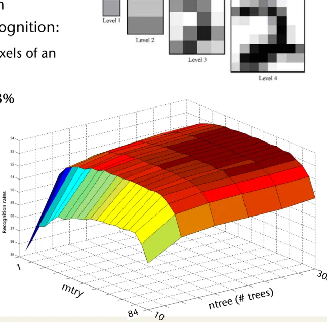
§  Other experiments on

handwritten digit recognition:

§  Feature vector = all pixels of an image pyramid

§  Recognition rate: ~ 93%

§  Dependence of recognition rate on ntree and mtry:

detail our experimental protocol in the following section.

3. Experiments

The idea of our experiments is to tune the RF main parameters in order to analyse the ”correlation” between the RF performances and the parameter values.

In this section, we first detail the parameters studied in our experiments and we explain the way they have been tuned. We then present our experiment protocol, by de- scribing the MNIST database, the test procedure, the results recorded and the features extraction technique used.

3.1. Parameters

As mentioned above, we tuned the two parameters of the Forest-RI method in our experiments : the number L of trees in the forest, and the numberKof random features pre-selected in the splitting process. In [3] Breiman states thatK has to be greater than 1, in which case the splitting variable would be totally randomly selected, but does not have to increase so much. Our experiments aim at progres- sively increasing this value to highlight whether or not this statement is true. Breiman also decides for his experiments to arbitrarily fix the number of trees to 100 for the Forest-RI algorithm. Thus, another goal of this work is to study the behavior of the method according to the number of trees, so that we would be able to distinguish a global tendency. As RF training process is quite fast, a wide range of trees can be grown inside the forest.

Consequently, we have drawn two ranges of values forK andL. Concerning the numberLof trees, we have picked six increasing values, from 10 to 300 trees. They have been chosen according to the global tendency that appeared during the experiments. Using less than 10 trees has proven to be useless, as well as increasing the number of trees be- yond 300 trees does not influence the convergence of the recognition rate.

Concerning the number of features we have tested 20 values following the same approach. This time small values have proven to be more interesting for seeing the global tendency of the recognition rate. Thus we have tested each value ofK from 1 to 16, and then five more greater values from 20 to 84.

3.2. Experimental protocol

The handwritten digit MNIST database is made of 60,000 training samples and 10,000 test samples [12]. The digits have been size-normalized and centered in a fixed- size image. It is a good database for people who want to try learning techniques and pattern recognition methods on

real-world data while spending minimal efforts on prepro- cessing and formatting.

In this experiment we would like to have an idea of the result variabilities. We have therefore divided the original training set into five training subsets of 10,000 samples. Let Ls denote the original 60,000 samples training set and T_s the 10,000 samples test set. We denote byL_s_i each of the 5 learning subsets. In Ls the classes are not equally rep- resented, that is to say that some of them contain less than 6,000 samples. However we would like to use strictly bal- anced training sets, i.e. training sets with equally distributed classes. We have consequently decided to use only five subsets instead of six. Moreover it has allowed us to reduce the tree-structure complexities.

The Forest-RI algorithm has been run with each couple of parameters on the fiveLsitraining sets, so that a RF was grown for one couple of parameters associated to oneL_s_i. Results on each run have been obtained by testing on theTs

set. Consequently we have obtained five recognition rates for each couple of parameters, for which we have computed the mean value. By recognition rate we mean the percent- age of correctly classified instances among all the test set samples, obtained with the forest built in the training stage.

With this work, our aim was not to discuss the influence of the feature quality on the performance of the classifier nor searching for best intrinsic performance. Our aim is rather to understand the role of the parameter values on the behavior of the RF. That is why we have decided to arbitrarily choose a commonly used feature extraction technique based on a greyscale multi-resolution pyramid [14].

We have extracted for each image of our set, 84 greyscale mean values based on four resolution levels of the image, as illustrated in figure 1.

Figure 1. Example of multiresolution pyramid of greyscale values of an image

The results and tendencies are discussed in the following section.

hal-00436372, version 1 - 26 Nov 2009

ntree (# trees)

1

84

(20)

Body Tracking Using Depth Images (Kinect)

§  The tracking / data ﬂow pipeline:

Infer body parts

per pixel Cluster pixels to hypothesize

body joint positions Capture

depth image &

remove bg

Fit model &

track skeleton

[Shotton et al.: Real-Time Human Pose Recognition in Parts from Single Depth Images; CVPR 2011 ]

(21)

The Training Data

Record mocap

500k frames

distilled to 100k poses

Retarget to several models

Render (depth, body parts) pairs

(22)

Synthetic vs Real Data

synthetic (train & test)

real (test)

For each pixel in the depth image, we know its correct class (= label).

Sometimes, such data is also called ground truth data.

(23)

Classifying Pixels

§  Goal: for each pixel determine the most likely body part (head, shoulder, knee, etc.) it belongs to

§  Classifying pixels =

compute probability P( c

_x

) for pixel x = (x,y),

where c

_x

= body part

§  Task: learn classiﬁer

that returns the most likely body part class c

_x

for

every pixel x

image windows move

with classiﬁer

(24)

Fast Depth Image Features

§   For a given pixel, consider all depth comparisons inside a window

§  The feature vector for a pixel x are all feature variables obtained by all

possible depth comparisons inside the window:

where D = depth image, 𝛥 = ( 𝛥

_x

, 𝛥

_y

) = offset vector,

and D(background) = large constant

§  Note: scale 𝛥 by 1/depth of x, so that the window shrinks with distance

§   Features are very fast to compute

input depth image

x

Δ

x

Δ

x

Δ

x

Δ

x

Δ

x

Δ

f (x, ) = D (x) D (x +

D (x) )

(25)

Training of a Single Decision Tree

§  The training set (conceptually): all features (= all f(x, 𝛥 ) ) of all pixels (= feature vectors) of all training images, together with the correct labels

§  Training a decision tree amounts to ﬁnding that 𝛥 and

^θ

such that the information gain is maximized

L

no yes

c P_r(c)

body part c P(c)

c P_l(c)

l r

L = { feature vectors ( f(x, 𝛥₁), …, f(x, 𝛥_p) ) with labels c(x) }

f (x, ) > ✓

L^l L^r

(26)

Classiﬁcation of a Pixel At Runtime

§  Toy example: distinguish left (L) and right (R) sides of the body

§  Note: each node only needs to store 𝛥 and

^θ!

§  For every pixel x in the depth image, we traverse the DT:

L R P(c)

no yes

f (x,

₁

) > ✓

₁

f (x,

₂

) > ✓

₂

(27)

Training a Random Forest

§  Train ntree many trees, for each one introduce lots of randomization:

§  Random subset of pixels of the training images (~ 2000)

§  At each node to be trained, choose a random set of mtry many (𝛥,^θ) values

§  Note: the complete feature vector is

never explicitly constructed (only conceptually)

ground truth

1 tree 3 trees 6 trees

inferred body parts (most likely)

40%

45%

50%

55%

1 2 3 4 5 6

Average per-class accuracy

Number of trees

(28)

§  Depth of trees: check whether it is really best to grow all DTs in the RF to their maximum depth

30%

35%

40%

45%

50%

55%

60%

65%

8 12 16 20

Maximum depth of trees

900k training images 15k training images

(29)

More Parameters

30%

32%

34%

36%

38%

40%

42%

44%

46%

48%

50%

0 50 100 150 200 250 300

Maximum probe offset (pixel meters)

31 63 129 195 260 ground

truth

10%

20%

30%

40%

50%

60%

10 100 1,000 10,000 100,000 1,000,000

Average per-‐class accuracy

Synthetic test set Real test set

Number of training images (log scale)

(30)

Implementing Decision Trees and Forests on a GPU - Sharp, ECCV 2008 Papers/Massively\ Parallel\ Algorithms/Random\ Forests

(31)

"The Wisdom of Crowds"