Optimal Financing Structures

(1)

Optimal Financing Structures

Inauguraldissertation zur Erlangung des Doktorgrades der Wirtschafts- und Sozialwissenschaftlichen Fakult¨ at der Universit¨ at zu K¨ oln

2018

vorgelegt von

Dr. rer. nat. Raphael Flore M.Sc.

aus Warburg

(2)

Tag der Promotion: 7.11.2018

(3)

Danksagung

Auf dem Weg zu dieser Dissertation hatte ich das große Glück, dass mir Möglichkeiten eingeräumt wurden, die nicht selbstverständlich waren. Angefangen hat dies mit der Möglichkeit als Quereinsteiger aus der Physik ein Promotionsstudium der VWL beginnen zu können. Für diese Offenheit bin ich der CGS sehr dankbar. Während ich mich anfangs im neuen Fach erst einmal orientieren musste, hatte ich das Glück mit Felix Bierbrauer einen Betreuer gefunden zu haben, der mir große Freiheit einräumte meine Interessen zu erkunden und meine eigenen Forschungsthemen zu entwickeln. Ich möchte ihm daher sehr danken für das mir entgegengebrachte Vertrauen und für das Engagement sich immer wieder in meine Arbeiten hinein zu denken, um mir sehr hilfreiche Kommentare zu geben.

Als sich meine Forschung immer mehr der theoretischen Finanzökonomie zuwandte, hatte ich schließlich das Glück, dass sich mit Martin Hellwig ein zweiter Betreuer meiner Promo- tion angenommen hat, der über eine herausragende Kenntnis dieses Fachgebiets verfügt.

Ich möchte ihm daher sehr danken für sein Interesse an meiner Arbeit und für die vielen Gespräche und Ratschläge, die außerordentlich wertvoll für mich waren.

Darüber hinaus möchte ich mich auch bei den Institutionen bedanken, an denen ich in den vergangenen Jahren Gast sein durfte und die mir die Möglichkeit gegeben haben an einem spannenden Austausch über finanzökonomische Fragen Teil zu haben. Hierfür möchte ich dem MPI zur Erforschung von Gemeinschaftsgütern, dem Finance Depart- ment der NYU Stern, der Finance-Gruppe an der Universität Bonn und Prof. Krahnen

& seinem Lehrstuhl an der Universit¨at Frankfurt danken.

Ebenso möchte ich mich aber auch bei meinen Kollegen am CMR in Köln bedanken, mit denen ich sehr viele interessante Gespräche über die Forschung führen konnte. Dabei ging es nicht nur um Themen, die in dieser Dissertation angesprochen werden, son- dern insbesondere auch um andere spannende Fragen der Volkswirtschaftslehre. Diese Gespräche haben mir sehr geholfen mich in meiner neuen Forschungsdisziplin einzuleben, und dafür möchte ich, neben einigen anderen, vor allem folgenden Personen danken: Mar- ius Vogel, Paul Schempp, Jann Goedecke, Christopher Busch, Jonas Löbbing, Thorsten Louis, Robert Scherf, Martin Scheffel, Christoph Kaufmann, Emanuel Hansen, Fabian Becker, Cornelius Schneider, Christian Bredemeier, Peter Funk, Michael Krause.

Und schließlich m¨ochte ich mich noch von ganzen Herzen bei meiner Familie und meinen Freunden bedanken, die mir die Kraft und die Lebensfreude gegeben haben, um diese Arbeit zu vollbringen.

(4)

(5)

1. General Introduction

The theory of corporate finance focuses on the optimal capital structure of a firm in a given environment: the firm chooses how to finance a given set of assets by selling financial claims to a given set of potential buyers. This dissertation extends the theory of corporate finance by accounting for the fact that both, the set of available assets as well as the demand for claims, can be altered by other firms and investment funds which buy and sell financial claims.

The following three chapters illustrate different implications of this extension. Chapters 2 and 3 take the assets as given, but study the emergence of intermediation chains: instead of choosing the capital structure that would be optimal if only retail investors bought financial claims, firms can benefit from selling a different composition of debt claims to funds or other firms, which finance these securities by selling their own debt to retail investors. Studying this possibility, the two chapters can explain the existence and some characteristics of intermediation chains that have emerged in financial markets in recent decades. Chapter 4 relaxes the assumption that a firm’s set of assets is given and allows firms to buy financial assets created by other agents in the market. The chapter shows how the possibility to buy financial assets challenges common notions about the optimal capital structure of a firm. It thereby addresses an issue of particular importance for the regulation of banks: the supposed costs of capital requirements.

An objective of all three chapters is to provide a better understanding of changes in the financial structure of banks and other intermediaries. This includes a better understanding of both, causes for changes that have occurred in recent decades as well as consequences of changes that can be enforced by regulation. In this way, the dissertation contributes to the ongoing debates about the regulation of banks and financial markets.

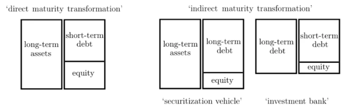
Abstract of Chapter 2: This chapter compares ‘direct maturity transformations’, in which risky long-term assets are directly financed with short-term debt, with ‘indirect maturity transformations’, in which such assets are financed with long-term debt that is financed with short-term debt in a second, separate step. (An example of the latter is the financing of senior tranches of securitized assets with short-term debt.) I show that the default probability of the short-term debt is higher in case of an indirect maturity transformation than in case of a direct transformation, given the same assets and the same level of short-term debt. If the purpose of short-term debt is the provision of ‘money-like’ claims,

(8)

indirect maturity transformations can be efficient in spite of the higher solvency risk, because long-term debt securities are more liquid than the underlying assets. But indirect maturity transformations can also emerge as form of regulatory arbitrage, if there is a public insurance of short-term debt and indirect maturity transformations are not subject to higher capital requirements than direct transformations.

Abstract of Chapter 3: This chapter provides an explanation for intermediation chains with stepwise maturity transformation, which have become a common form of financial intermediation. (An example are banks with long-term assets that sell commercial paper with month-long duration to money market funds that are financed by daily demandable shares). The explanation reconciles the idea of debt as disciplining device with the idea of safe debt as ‘money-like’ claim. The chapter shows that these two purposes of debt financing lead to conflicting predictions of the optimal level and the optimal duration of bank debt. This conflict can be resolved by a partial separation of the two purposes: the bank chooses the capital structure that optimizes the disciplining of its managers, while it sells some of its debt to a fund that provides money-like claims, which are backed by the bank debt.

Abstract of Chapter 4: Trade-off theories of capital structure describe how a firm chooses its leverage for a given set of assets. This chapter studies how the predictions of such theories change if one accounts for the possibility that firms can invest in financial markets.

Studying four different trade-off theories, the chapter shows for each of them: given any set of firm assets and the corresponding optimal capital structure, the firm can reduce its leverage and its insolvency risk relative to this supposed optimum without a loss of value, if it ‘integrates a fund’ – i.e., if it issues additional equity in order to buy financial assets with certain properties. The chapter thus indicates a way how the leverage and the insolvency risk of banks can be reduced without any costs in the long run.

(9)

2. Indirect Maturity Transformations

2.1. Introduction

Maturity transformations are a key aspect of financial intermediation and have received a lot of attention in the banking literature. The description of maturity transformations usually refers to a financial firm that has long-term assets and finances these with short- term debt. Quite often, however, financial intermediation entails an additional layer: in a first step, long-term assets are financed with long-term debt, and this long-term debt is financed with short-term debt in a second step. A prominent example, which played a key role in the Financial Crisis 07/08, is the securitization of loans and the purchase of the resulting tranches by banks or funds that are financed with short-term debt.¹ This form of maturity transformation is ‘indirect’ in the sense that the short-term debt claims refer to the underlying long-term assets only indirectly, via another financial claim that has a long duration. The contribution of this chapter is to provide a comparison of such indirect maturity transformations (IMT) with the direct maturity transformations (DMT) indicated above, in which the short-term debt is directly issued by the firm that holds the long-term assets. In particular, I compare the stability of IMT and DMT, measured in terms of the default probability of short-term debt. And I discuss why the different forms of maturity transformation can emerge. Based on this analysis, I derive implications for the regulation of financial intermediation that involves IMT.

Consider an IMT in which a set of assets is financed with equity as well as long-term debt. The long-term debt is senior to the equity at its maturity date. At intermediate dates, however, the value of the long-term debt can decrease due to an increase in the conditional probability of default at maturity, while the equity maintains a strictly positive value owing to the remaining probability that the asset payoff is larger than the debt liability at its maturity. This property leads to different default probabilities of short-term debt for IMT and DMT. In case of an IMT, in which the long-term debt is financed with short-term debt whose face value is D, the short-term debt defaults in states in which the value of the long-term debt falls belowD. In some of these states, however, the value of the underlying assets can be larger than the value of the long-term debt and larger than D, so that the same level of short-term debt would not default in case of DMT.

The difference between the value of the long-term debt and the value of the underlying

1Cf. Pozsar et al. (2016), for instance.

(10)

assets is given by the equity value in the first step of the IMT. The equity in that step can maintain a strictly positive value while the short-term debt in the second step defaults.

The result is: given the same underlying assets and the same level of short-term debt, the default probability of the short-term debt is higher in case of IMT than in case of DMT.

Or put differently, IMT require larger amounts of equity than DMT in order to avoid a default of the short-term debt.

The difference in default probabilities between IMT and DMT follows directly from the characteristics of debt contracts and does not depend on any specific assumptions or frictions. But it also holds true and it is economically relevant, if one accounts for common frictions of financial intermediation. Consider a situation with the following two features:

first, the selection and operation of assets is subject to moral hazard, which can be over- come if the agent who selects and operates the assets retains a sufficiently large equity claim to these assets (as suggested by Gorton & Pennacchi (1995) or Cerasi & Rochet (2012), for instance); second, investors pay a premium for safe debt claims, because they can use these claims similarly to money as a means of payment (as pointed out by Gorton

& Pennacchi (1990)). In liquid markets, debt is safe if there is no risk that the value of the underlying portfolio is smaller than the face value of the debt at the maturity date.

And since the value of a portfolio can fall less over a short duration than over a long duration, debt with a short duration allows for providing a higher level of safe, ‘money-like’

claims. DMT allow to finance assets with the maximally possible level of safe short-term debt, while a retention of equity by the selector of the assets ensures that good assets are chosen. In case of IMT, the selector must also retain some equity for this purpose, but sells long-term debt to a bank or fund. In order to obtain a premium for money-like claims, this bank or fund can also finance this purchase with safe short-term debt. For the reasons mentioned above, however, the level of safe short-term debt and the related premium are smaller for IMT than for DMT.

Given this disadvantage of IMT relative to DMT in providing money-like claims, one has to wonder why IMT emerge. While the disadvantage is due to a higher solvency risk, IMT can have a relative advantage owing to a decrease in liquidity risk. If the assets and capital markets are illiquid, the liquidation or refinancing of a portfolio at intermediate dates might only be possible at depressed prices. This risk of a depressed portfolio value constrains the level of safe, money-like claims that can be issued against the portfolio. As highlighted by Shleifer & Vishny (1992), one aspect of illiquidity is that selling assets to new owners can entail a loss of specialized skills in operating the assets. In this respect, a long-term debt claim to a set of assets is more liquid than the underlying assets, because a sale of the debt only transfers a passive claim without changing the operator of the assets. While the short-term debt in case of DMT refers directly to the assets, the short-term debt in case of IMT refers to the more liquid long-term debt claims. The level of safe short-term debt in case of IMT is thus less constrained by liquidity risk than in

(11)

2.1. Introduction case of DMT. If the relative decrease in liquidity risk is larger than the relative increase in solvency risk, then IMT allow for providing more safe short-term debt than DMT. And given a premium for such money-like claims, there is an incentive to finance assets with IMT instead of DMT.

Besides rationalizing the emergence of IMT, the explanation just given contains a novel argument for an increase of liquidity by securitization: while assets can be illiquid, because their operation requires skills that are not perfectly transferable (like, for instance, lend- ing relationsships with households or firms), a long-term debt security is just a financial claim whose transfer does not affect the operation of the underlying assets. Previous arguments for an increase of liquidity by securitization (as presented in DeMarzo (2005), for instance) have highlighted that an appropriate security design reduces adverse selection and maximizes the profit of an agent who sells some claims to assets, while maintaining the remainder. Arguments based on adverse selection, however, cannot explain why the payoff from liquidating the entire set of assets (which is the upper bound for safe debt in case of DMT) is smaller than the payoff from selling a long-term debt claim to these assets (which is the upper bound for safe debt in case of IMT). These arguments can thus not rationalize the emergence of IMT in a similar way as this chapter does.

The explanation for IMT given above applies to segments of financial markets that have no access to a public insurance of short-term debt (like a deposit insurance, for instance).

Such an insurance negates the relative advantage of IMT that is based on a decrease of liquidity risk. To avoid moral hazard, however, insurance premiums or capital requirements are required to prevent that solvency risk can be shifted to the insurance. Since the solvency risk in higher for IMT than for DMT, the capital requirements or insurance premiums have to be larger for IMT than for DMT. If such requirements or premiums are imposed, there is no incentive for financial firms to engage in IMT instead of DMT, because it implies higher costs (i.e., higher insurance premiums or a lower level of money- like claims as consequence of higher capital requirements), while the relative advantage of IMT is lost (the relatively smaller liquidity risk). This contrast with a situation in which the same capital requirements apply to DMT and IMT, which means that the same lower bound for equity is imposed to both modes of intermediation. In that case, IMT can be privately optimal owing to an implicit subsidy by the insurance: given the higher solvency risk of IMT, the same level of equity in both modes implies that the insurance covers some solvency risk in case of IMT that is not covered in case of DMT. The policy implication of the analysis is thus: if a public authority provides an insurance of short-term debt in order to improve the provision of money-like claims, but it wants to avoid an implicit subsidization of IMT, then it should impose higher capital requirements in case of IMT than in case of DMT.

Additional related literature: There are some recent papers that analyze financial intermediation which is performed in different steps. Allen et al. (2015) and Gale &

(12)

Gottardi (2017), for instance, analyze the optimal distribution of equity between firms and banks that lend to these firms. But they do not address maturity transformations and focus on issues like diversification and bankruptcy costs instead. Flore (2018) [which is identical with Chapter 3 of this dissertation] also studies maturity transformations that involve more than one step. But that paper focuses on the division of maturity transformation into smaller steps, which means that long-term assets or securities are financed with medium-term debt which is then financed with short-term debt. The literature on financial networks, following Allen & Gale (2000) and Freixas et al. (2000), also studies financial intermediation that involves more than one step. This literature, however, has not noted the differences between IMT and DMT and its consequences. The same holds for the literature that studies regulatory differences between traditional banks and more recent forms of financial intermediation, with Hanson et al. (2015), Plantin (2015), Flore (2015), Luck & Schempp (2014,2016) as examples for theoretical papers in this area.

Theremainder of this chapteris structured as follows: Section 2 shows that IMT lead to a higher default probability than DMT. Section 3 illustrates that this difference has relevant implications for the optimal form of financial intermediation. Section 4 provides a rationale for IMT by highlighting its positive effect on liquidity risk. Section 5 discusses the regulation of IMT in case of an insurance of the short-term debt.

2.2. The Basic Mechanism

This section derives the key result of this chapter, which is: an indirect maturity transformation, in which assets are financed with long-term debt that is financed with short-term debt in a second step, implies a higher default probability than a direct maturity transformation, in which assets are directly financed with short-term debt. This result is a direct consequence of the contractual properties of debt claims.

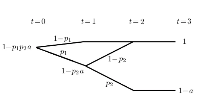
Consider three dates t = 0,1,2 and two types of agents: first, an ‘asset operator’ who needs the external fundingI for her assets att = 0, which she can obtain by issuing equity and debt claims; second, a continuum S_I of ‘investors’ whose wealth at t = 0 adds up to W_I > I and who can either invest in a storage technology with zero return or who can buy financial claims from the asset operator or from each other. For simplicity, I start with the assumption that all agents are risk-neutral and simply want to maximize their expected wealth att= 2. The investors thus buy a financial claim as long as its expected return is weakly larger than the benchmark rater= 0 set by the storage technology. (Be- low Proposition 1, I explain why the results also holds for more general risk preferences.) The assets have the stochastic values ˜x₁ at t = 1 and ˜x₂ at t = 2, which are distributed according to the density functions f₁ and f₂, and which constitute a martingale process:

E [˜x₂|˜x₁] = ˜x₁. For simplicity, assume that f₁(x₁) and f₂(x₂|x₁) are continuous functions

(13)

2.2. The Basic Mechanism of x₁. (The proof of Proposition 1 shows how the results can be generalized.)

In this section, I just study the properties of the equity and debt claims that can be issued with direct or indirect reference to these assets. The optimal choice of financing, given these properties, is examined in the next section. The case that the asset operator sells debt that matures att= 1 is called ‘direct maturity transformation’ (DMT) and the respective face value of the ‘short-term’ debt is denoted as D_S. Assume that the assets are perfectly liquid, so that they yield the payoff x₁ in case of a liquidation at t = 1.

(Illiquidity will be discussed in Section 2.4.) A default of the short-term debt can then be defined as the occurrence of x₁ < D_S, which implies a default probability φ_D(D_S) equal to E [˜x₁ < D_S]. The valuee_D(D_S) of the equity att= 0 is given by the expected residual payoff E [max{˜x₁−D_S,0}].

Compare this to the case that the asset operator sells ‘long-term’ debt which matures at t = 2 and which has a face value D_L. I refer to this choice of financing by calling it

‘securitization vehicle’. The value e_V(D_L) of the equity of the securitization vehicle at t = 0 is given by the expected residual payoff E [max{˜x₂−D_L,0}]. Consider now that one of the investors buys this long-term debt and finances the purchase by selling equity and short-term debt that is backed by the long-term debt security. The face value of this short-term debt shall be denoted as DÎ_S and I refer to this financing of the long- term debt security as ‘investment bank’. The value ˜y₁ of the long-term debt at t = 1 is the expected payoff of the D_L-claim conditional on the value ˜x₁ of the underlying assets: ˜y1(DL) = E [min{˜x2, DL}|˜x1]. Defining a default of the investment bank’s short- term debt as the occurrence of y₁(D_L) < DÎ_S, the default probability φ_I(D_SÎ, D_L) equals E

˜

y₁(D_L)< D_S^I

. The valuee_I(D^I_S, D_L) of the investment bank’s equity att= 0 is given by the expected residual payoff E

max{˜y₁(D_L)−D_S^I,0}

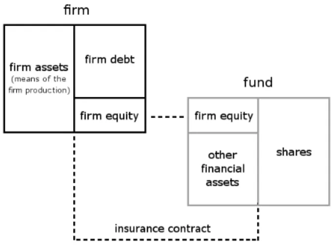
. The combination of securitization vehicle and investment bank is called ‘indirect maturity transformation’ (IMT), because the short-term debt refers to the underlying long-term assets indirectly, via the long-term debt claim. The two ways of maturity transformation are depicted in Fig. 2.1.

Figure 2.1.: Schematic balance sheets of two different ways of maturity transformation.

(14)

Observation 1

Despite the seniority of the long-term debt at t= 2, the value of the long-term debt can decline att= 1, while the equity value of the securitization vehicle remains strictly positive:

∃x₁, D_L∈R⁺: E[max{˜x₂−D_L,0}|x₁]>0∧y₁ =E[min{˜x₂, D_L}|x₁]<E[min{˜x₂, D_L}].

If this holds for the lowest asset value att= 1, which means forx₁=x_S,min:= min(supp(f₁)), then the lowest possible value y_S,min of the long-term debt at t = 1 is smaller than the lowest possible value of the underlying assets: y_S,min ≤E[min{˜x₂, D_L}|x_S,min]< x_S,min. These properties have consequences for the short-term debt capacity of the two modes of maturity transformation:

Proposition 1

a) Given the same assets and the same level of short-term debt, the default probability is larger for IMT than for DMT:

φ_I(D_S^I, D_L)≥φ_D(D_S) ∀ D^I_S =D_S ∈R⁺ and D_L∈R⁺,

with strict inequality if D_S^I =D_S ∈supp(f₁) and D_L <max supp(f₂(x₂|x₁ =D_S^I) . b) Given the same assets and the same initial level of equity, the default probability is larger for IMT than for DMT:

φ_I(D_SÎ, D_L)≥φ_D(D_S) ∀ D_SÎ, D_S, D_L∈R⁺ s.t. e_I(DÎ_S, D_L) +e_V(D_L) =e_D(D_S), with strict inequality if D_SÎ ∈supp(f₁) and D_L<max supp(f₂(x₂|x₁ =DÎ_S)

. Intuition: Before I present the proof, let me give a brief intuition. Short-term in both cases, DMT and IMT, defaults att = 1, if the value of the underlying portfolio is less than the debt face value. The default probability is weakly higher for IMT than for DMT, since the value of the long-term debt att = 1 is weakly smaller than the value of the underlying assets. The difference is given by the value of the equity of the securitization vehicle. This equity can maintain a strictly positive value even in states at t = 1 in which the value of the long-term debt has declined due to an increase in the conditional probability of low payoffs. Consequently, there are debt levels for which the asset value E [˜x₂|x₁] = x₁ remains larger thanD_S =D^I_S in some statesx₁, while the value E [min{˜x₂, D_L}|x₁] of the long-term debt falls belowD^I_S. The remaining equity value E [max{˜x₂−D_L,0}|x₁] of the securitization vehicle does not prevent the default of the investment bank’s short-term debt. The equity of the investment bank or the asset operator is strictly junior to the short-term debt, so that the debt only incurs a loss at t = 1, if the equity value has fallen to zero by ‘absorbing’ losses of the portfolio. This does not hold for the equity of the securitization vehicle. As a result, given the same level of equity (e_V +e_I = e_D), the equity in case of IMT is less effective in preventing short-term debt default than the equity in case of DMT.

(15)

2.2. The Basic Mechanism

Proofs: Proof of statement a):

φ_I(D_S^I, D_L) = E

˜

y₁(D_L)< D^I_S

= E

E [min{˜x₂, D_L}|˜x₁]< D_S^I

≥E

˜

x₁< D^I_S

=φ_D(D_S^I).

The inequality is strict forD_SÎ=D_S∈supp(f₁) andD_L<max supp(f₂(x₂|x₁=DÎ_S) , since there are states at t = 1 in which the asset value x₁ is weakly larger than D_SÎ = D_S ∈ supp(f₁) (which thus do not contribute to E

˜

x₁ < D_S^I

), while the value E [min{x˜₂, D_L}|x₁] = x₁−E [max{˜x₂−D_L,0}|x₁] of the long-term debt is smaller thanx₁ and smaller thanD^I_S (so that the states contribute to E

E [min{x˜2, DL}|˜x1]< D_S^I

). The set of states with this property has non-vanishing mass due to the continuity off1(x1) andf2(x2|x1) as functions of x₁.

Without imposing these assumptions onf₁andf₂, one can generalize the result as follows:

the inequality is strict for allD^I_S =D_S ∈R⁺\∞andD_L∈R⁺\∞, for which there is a subset Ω⊂supp(f₁) with non-vanishing mass such thatD^I_S ∈ ∩_x₁∈Ω E [min{˜x₂, D_L}|x₁], x₁

. Proof of statement b): the same level of equity in IMT and DMT means that

eD(DS) = eV(DL) +eI(D^I_S, DL) E [max{˜x₁−D_S,0}] = E [max{˜x₂−D_L,0}]+E

max{˜y₁(D_L)−D_S^I,0}

= E [max{˜x₂−D_L,0}]+E

max{E [min{˜x₂, D_L}|x˜₁]−D^I_S,0}

= E [max{˜x₂−D_L,0}]+E

max{˜x₁−E [max{˜x₂−D_L,0}|˜x₁]−D_S^I,0}

≥E [max{˜x₂−D_L,0}]+E

max{˜x₁−D_S^I,0}

−E [E [max{˜x₂−D_L,0}|˜x₁]]

= E

max{˜x1−D^I_S,0}

The inequality is strict for D_S^I ∈supp(f1) and DL<max supp(f2(x2|x1 =D^I_S)

, because there are states att = 1 in which the asset valuex1 is weakly smaller than D_S^I ∈supp(f1) (so that max

x₁−D_S^I,0 and max

x₁−E [max{x˜₂−D_L,0}|x₁]−D^I_S,0 are both equal to zero), while the value E [max{˜x₂−D_L,0}|x₁] is strictly positive. The set of states with this property has non-vanishing mass owing to the continuity of f₁(x₁) and f₂(x₂|x₁) as functions of x₁. The inequality E [max{˜x₁−D_S,0}] ≥ E

implies E [˜x₁< D_S]≤E

˜

x₁< D_S^I

and thus:

φ_D(D_S) = E [˜x₁<D_S]≤E

˜ x₁<D_S^I

≤E

E [min{˜x₂, D_L}|˜x₁]< D_S^I

=φ_I(D_S^I,D_L). (2.1) A strict inequality E [max{˜x₁−D_S,0}] > E

implies a strict inequality φ_D(D_S) < φ_I(DÎ_S, D_L). Without assumptions about f₁ and f₂, one can generalize the result in the same way as in a): the inequalityφ_I(D_SÎ, D_L)≥φ_D(D_S) is strict for all cases withe_I(DÎ_S, D_L) +e_V(D_L) = e_D(D_S), for which there is a subset Ω⊂supp(f₁) with non- vanishing mass such that D_SÎ ∈ ∩_x₁∈Ω E [min{˜x₂, D_L}|x₁], x₁

. If this holds, the second

(16)

inequality in Eq. (2.1) is strict, even if the first inequality is not.²

Generalized Pricing: Let me briefly indicate why the results are robust to any pricing of the claims which is monotonously increasing in payoffs at t = 2. The basic intuition remains the same: the assets are a more valuable backing of short-term debt than a long-term debt claim to the assets, since some payoff of the assets accrue to the equity of the securitization vehicle. The pricing of claims enter the analysis by the valuation of the initial equity as well as the liquidation values of the assets and the long-term debt security at t = 1. Let us denote the latter two as v^L_A and v_D^L and consider that these values are not simply given by y₁(D_L) and x₁, which means by the expected payoff at t = 2, but by more general weighted sums of the payoffs at t = 2:

v^L_D = R

ν(min{x₂(ω), D_L}, ω)ρ(ω, x₁)dω and v_A^L = R

ν(x₂(ω), ω) ρ(ω, x₁)dω, where ω is an index of states at t = 2 with respective asset payoff x₂(ω), while ρ(ω, x₁) is the probability of a state ω conditional on x₁ and ν(p, ω) is the valuation of a payoff p in state ω. In liquid markets, the default probabilities generalize toφ_D(D_S) = E

v_A^L < D_S and φ_I(D^I_S, D_L) = E

v_D^L < D^I_S

. Statement a) in Proposition 1 is robust to such generalization, since v_D^L =R

ν(min{x2(ω), DL}, ω) ρ(ω, x1)dω ≤R

ν(x2(ω), ω) ρ(ω, x1)dω =v_A^L holds for any valuation ν that is monotonously increasing in the payoff at t= 2. And the inequality is strict for someD_L. Following the same logic, the valuation of equity att= 0 can be generalized and it can be shown that the statement b) in Proposition 1 is robust to such generalization, given monotonous pricing.

Corollary 1

For a given amount of initial equity in IMT (i.e., e_V(D_L) +e_I(D^I_S, D_L) =const.), the default probability of the short-term debt increases with the amounte_V(D_L) =E[max{˜x₂−D_L,0}]

of this equity that is issued by the securitization vehicle, which means that it decreases with the level D_L of the long-term debt:

d dD_L

eI(D^I_S,DL)+eV(DL)=const.

φ_I(D_S^I, D_L)≤0.

If the securitization vehicle has no equity, but only long-term debt, the default probability does not differ from DMT:

e_V(D_L) = 0⇔D_L= max(supp(f₂))⇒φ_I(DÎ_S, D_L) =φ_D(D_S) ∀ D_S =DÎ_S ∈R⁺. These statements follow fromφ_I(DÎ_S, D_L) = E

˜

y₁(D_L)< D_S^I

= E

E [min{˜x₂, D_L}|˜x₁]< D^I_S , which decreases in DL and which is equal to E

˜

x1 < D^I_S

for DL = max(supp(f2)). The overall equity level eV(DL) +eI(D_S^I, DL) remains fixed in spite of an increase in DL and

2Alternatively, the result can also be generalized as follows: the inequality φ_I(DÎ_S, D_L)≥ φ_D(D_S) is strict for all cases with e_I(DÎ_S, D_L) +e_V(D_L) =e_D(D_S), for which there is a subset Ω⁰ ⊂supp(f₁) with non-vanishing mass such thatDÎ_S < x₁ and E [max{x˜₂−D_L,0}|x₁]>0 for allx₁∈Ω⁰.

(17)

2.3. Relevance for Financial Intermediation a corresponding decrease in e_V(D_L), if e_I(D_S^I, D_L) = E

max{y˜₁(D_L)−D_S^I,0}

increases owing to an decrease inD^I_S. This contributes to the decrease inφ_I(D_S^I, D_L), too. The case DL = max(supp(f2)), however, is degenerate in the sense that the distinction between equity and debt vanishes. The securitization vehicle only sells a single claim that receives the entire payoff of the assets and that is held by the investment bank. The investment bank thus completely ‘owns’ the securitization vehicle and its assets.

To sum up, this section has shown that indirect maturity transformations (IMT), in which short-term debt refers to some asset payoff via long-term debt claims to the assets, imply higher default probabilities than direct maturity transformations (DMT), in which the short-term debt directly refers to the assets. IMT imply higher default probabilities than DMT for the same underlying assets and the same level of short-term debt or the same level of initial equity. This result does not depend on any frictions, but only on the basic contractual features of debt contracts.

2.3. Relevance for Financial Intermediation

This section shows that the difference identified in the previous section is strict and relevant in a setting in which agents choose the optimal financing of assets given two frictions that are well-established in the literature: first, a premium for safe claims which can be used as means of payment – as pointed out by Gorton & Pennacchi (1990); second, moral hazard concerning the operation or selection of assets, if claims to their payoff are sold – see Gorton & Pennacchi (1995), for instance. The first friction leads to a deviation from the Modigliani-Miller Theorem and can explain the use of short-term debt financing.

The second friction explains why the institution which selects or operates assets retains some claims to these assets. The two frictions are introduced in the next two subsections, before the third subsection discusses optimal financing given these frictions.

2.3.1. Risk Retention as Commitment Device

If the quality of the assets is not fixed, but depends on costly actions of the asset operator, the sale of claims to the asset payoff can lead to moral hazard. Consider the case that the asset operator can select ‘bad assets’ instead of the ‘good assets’ characterized by

˜

x_t. The stochastic value ˜x^b_t of these bad assets is also an martingale, but it is first-order stochastically dominated by the value ˜xt of the good assets at both dates t = 1,2. Let us assume that the asset operator has a private benefit µ from choosing bad assets (for instance, because a poorer screening of loans entails less costly effort), but the choice is inefficient due to µ <E [˜x₂]−E

˜ x^b₂

. As stressed by Gorton & Pennacchi (1995), among others, the asset operator can commit to choose the good assets, if she retains claims to the assets whose expected loss from choosing bad assets is weakly larger than µ.

(18)

Let us focus on the retention of equity as a commitment device, before I comment on the possibility to retain debt claims at the end of this section. The expected loss L_A(D_d;d) of the equity from choosing bad assets depends on the face value Dd and the duration d∈ {S, L} of the debt as follows

L^E_A(Dd;d) = E

max{˜x_T_(d)−Dd,0}

−E

max{˜x^b_T_(d)−Dd,0}

,

with the maturity dates T(S) = 1 and T(L) = 2. The boundary values L^E_A(0;d) = E

˜ x_T_(d)

−E h

˜ x^b_T_(d)

i

and L^E_A(∞;d) = 0 imply:

Observation 2

There are maximal debt levels for which the loss of equity from choosing bad assets is still larger than the private benefit: D^c_d:= max{D_d|L^E_A(D_d;d)≥µ} for d=S, L.

The asset operator has an incentive to retain a fractionγof the equity withγ L^E_A(D_d;d)≥ µ. If the asset operator retains a smaller fraction of the equity, it will be optimal for her to choose bad assets, independent of the price that investors pay for their claims. Taking this choice into account, however, the investors will only buy claims at prices that reflect their expected loss from bad assets. By means of this rational pricing the asset operator will thus incur the cost of choosing bad assets. If the asset operator retains a fraction γ ≥ _LE ^µ

A(Dd;d) of the equity, in contrast, choosing the good set is optimal for her and the investors account for this fact when they buy claims.

2.3.2. Safety Premium

Based on Gorton & Pennacchi (1990), I assume that the investors benefit from claims whose value is safe, because they can trade these claims without problems of asymmetric information, so that they constitute an efficient means of payment. Given this benefit of safe claims, investors accept to pay a premium for them. A microfoundation of this premium based on transaction needs of investors between t = 0 and t = 1 in presence of asymmetric information is given in Appendix A.1. For the questions addressed in this Chapter, however, it is sufficient to represent the benefits of claims with safe value in a simple way: by assuming that the investors pay a fee λ per unit of claim whose value is safe between t = 0 and t = 1.³ I will refer to these claims as ‘money-like claims’ and they are measured in terms of expected payoff. For simplicity, I assume that premium is paid at the very end, after the debt has been paid off at t= 2.⁴ Consequently, the safety

3One can think of fees like the ones paid for deposit accounts. Transaction needs and fees for safe claims in the second period have been considered in an earlier version of this Chapter (which can be provided on demand), but do not change the results qualitatively.

4This allows to ignore tedious, uninteresting effects of paid fees on the safety of the debt and the size of the premium. The assumption implies: even if investors withdraw their debt or transfer it in a payment process, they do not pay the fee for holding the safe claim (up to the withdrawal date) before the very end.

(19)

2.3. Relevance for Financial Intermediation premium Λ(D_d;d) that the asset operator earns by selling debt claims with face valueD_d and duration d is:

Λ(D_d;d) = λ·v_D(D_d;d) forD_d≤x_d,min and Λ(D_d;d) = 0 else, where v_D(D_d;d) = E

min{D_d,x˜_T_(d)}

is the value (i.e., the expected payoff) of the debt claim (which equalsD_d for safe debt), while x_d,min is defined as: x_S,min := min{suppf₁} (which is the lower bound of ˜x₁); and x_L,min:= max

D_L|E

min{D_L,x˜₂}

˜x₁

=const.

(which is highest possible face value of long-term debt whose expected payoff is independent of the state att= 1, which means that it is safe betweent = 0 andt = 1). I assume perfect liquidity of the assets in this section (i.e, a liquidation of the assets att= 1 would yield a payoff ˜x₁), before I account for asset illiquidity in Section 2.4. For simplicity, I assume that x_S,min and x_L,min remain the same, if one replaces ˜x_t with ˜x^b_t, which means that these bounds are the same for good and bad assets.⁵

If an investor sets up an investment bank, which means that she buys long-term debt of the asset operator and sells equity and debt claims to this long-term debt security, she can also earn a safety premium. For debt with face value D_d^I and duration d, the safety premium is:

ΛÎ(D_dÎ;d, D_L) =λ·vÎ_D(DÎ_d;d, D_L) forD_dÎ ≤y_d,min(D_L) and Λ(D_dÎ;d, D_L) = 0 else, (2.2) where y_d,min(D_L) is defined in the same way as x_d,min with ˜y_t(D_L) = E [min{D_L,x˜₂}|˜x_t] instead of ˜x_t.

Lemma 1

a) The safety premium is maximized by selling short-term debt:

argmax

Dd∈R⁺,d∈{S,L}

Λ(D_d;d) = (x_S,min, S), argmax

D^I_d∈R⁺,d∈{S,L}

Λ^I(D^I_d;d, D_L) = (y_S,min(D_L), S).

b) DMT allows for a larger premium than IMT: Λ(x_S,min;S)≥Λ^I(y_S,min(D_L);S, D_L), with strict inequality if D_L<max(supp(f₂|x₁=x_S,min)).

Proof: a) The martingale property of ˜x_t implies v_D(x_S,min, S) ≥ v_D(x_L,min, L) because: v_D(x_S,min, S) =x_S,min ≥ E [min{x_L,min,x˜₂}|x_S,min] = E [E [min{x_L,min,x˜₂}|˜x₁]] = v_D(x_L,min, L) (the second last equation follows from the definition of x_L,min). This means that (x_S,min, S) is the maximum of Λ(D_d;d). And the martingale property of ˜x_t implies that the value ˜y_t(D_L) of the long-term debt is a martingale, too:

5If one considered a downward shift of these bounds due to the selection of bad assets, the following results would be further strengthened, but their representation became more tedious. Owing to the stochastic dominance of ˜x₁ over ˜x^b₁, an upward shift is not possible forx_S,min(which will turn out to be the relevant bound).

(20)

E [˜y₂(D_L)|˜y₁(D_L)] = E [E [min{D_L,x˜₂}|˜x₂]|E [min{D_L,x˜₂}|˜x₁]] = E [min{D_L,x˜₂}|˜x₁] =

˜

y₁(D_L). Consequently, v_DÎ(y_S,min, S) ≥vÎ_D(y_L,min, L), so that (y_S,min, S) is the maximum of ΛÎ(DÎ_d;d).

b) Λ(x_S,min;S) = λ · x_S,min ≥ λ · y_S,min(D_L) = Λ^I(y_S,min(D_L);S, D_L) follows from

˜

x₁ ≥ E [min{D_L,x˜₂}|˜x₁] = ˜y₁(D_L). And D_L < max(supp(f₂|˜x₁ = x_S,min)) implies that x_S,min >E [min{D_L,x˜₂}|x_S,min] and thusx_S,min > y_S,min(D_L).

Intuition: a) If the value vD(DL;L) of a long-term debt claim is safe at t = 1, the expected payoff of the debt claim at t = 2 must be equal to vD(DL;L) conditional on each possible state at t = 1, including the worst possible one. This implies that the value of the underlying portfolio at t = 1 is weakly larger than v_D(D_L;L) in each possible state.

Since the level of safe short-term debt can be as high as the minimal possible value of the portfolio at t = 1, this implies that weakly more money-like claims can be provided by means of safe short-term debt than by long-term debt with safe value.

b) As shown in Section 2.2, the level of safe short-term debt is weakly larger in case of DMT than in case of IMT. As consequence of part a), the premium that can be earned for money-like claims is thus weakly larger for DMT than for IMT. The inequalities are strict, if short-term debt with face value D^I_S =xS,min is not safe in case of IMT, because the value y₁(D_L) of the long-term debt in the worst possible state at t = 1 is strictly smaller than the asset value x_S,min.

2.3.3. Optimal Financing in Presence of these Frictions

This subsection compares the optimal financing of assets given two possible modes of maturity transformations. Let us start with the optimal capital structure in case of DMT and consider the decision problem of the asset operator who wants to maximize her expected wealth. Selling claims to investors, she has no incentive to deviate from the investors’ reservation price for claims, which equals the expected payoff of the claim in case of risk-neutrality and a storage technology with zero return. This implies that the expected payoff P of the claims sold to investors has to be weakly larger than I in order to obtain the funding of the assets att = 0. Assume that, if the asset operator sells claims worth more than I, she can also store her wealth with zero return. Her expected wealth at t = 2 would thus be E [˜x2]−I, if there were no frictions. But the asset operator can earn the premium Λ(Dd;d) for money-like claims. And there is the potential loss from selecting bad assets: E [˜x₂]−E

˜ x^b₂

−µ

·1{^{µ>γ L}^EA(D_d;d)}. While the fractionγ of equity that is retained by the asset operator has no effect on Λ(D_d;d), it has a weakly positive effect on the moral hazard problem. It is thus always optimal for the asset operator to retain all of the equity, so that one can focus on γ = 1. The decision problem of the asset

(21)

2.3. Relevance for Financial Intermediation

operator is then:

max

Dd∈[0,1],d∈{S,L} X(D_d;d) + Λ(D_d;d) s.t. P(D_d)≥I with X(D_d;d) := E [˜x₂]−I− E [˜x₂]−E

˜ x^b₂

−µ

·1{^µ>L^EA(D_d;d)}. (2.3)

Assumption 1 x_S,min ≥I.

The purpose of this assumption is only to focus in a simple way on cases in which the funding I for the assets can be acquired, if the optimal capital structure is chosen. It applies to the remainder of this Chapter.

Lemma 2

The optimal capital structure consists of short-term debt with face value D^∗_S =x_S,min. Proof: P(D_S^∗)≥I, since the expected payoff of the safe claimD^∗_S isx_S,min. The objective function is maximized by short-term debt with D_S = x_S,min, because it maximizes Λ, whileL^E_A(D_S^∗;S) = E [max{˜x₁−x_S,min,0}]−E

max{˜x^b₁−x_S,min,0}

= E [˜x₁]−x_S,min− E

˜ x^b₁

+x_S,min ≥ µowing to E [˜x₁] = E [˜x₂], E

˜ x^b₁

= E

˜ x^b₂

. The second equality holds because x_S,min is the lower bound of both, ˜x₁ and ˜x^b₁.⁶

Intuition: Short-term debt financing is optimal, as it maximizes the amount of safe claims that can be provided to investors and on which a premium can be earned. And the retention of the equity claim by the asset operator ensures the efficient choice of good assets.

Having determined the optimal choice of financing which is possible with DMT, let us now study the possibility of IMT. The most profitable form of IMT can be characterized by the face valuesD_LandDÎ_S which maximize the sum of the investment bank’s premium ΛÎ(D_SÎ;S, D_L) and the expected payoff X(D_L;L) of the securitization vehicle. As shown in Lemma 1, ΛÎ(D_SÎ;S, D_L) is maximized by DÎ_S = y_S,min(D_L) for given D_L, and one can focus the discussion on that case. The potential safety premium Λ(D_L;L) of the securitization vehicle is neglected in the following comparison of IMT and DMT, because Λ(DL;L) would be paid by the investment bank, so that it would net out in the overall profit of securitization vehicle and investment bank.

Lemma 3

In the most profitable form of IMT, the equity level of the securitization vehicle is either just enough to ensure the selection of good assets (i.e.,D_L =D_L^c) or zero (i.e., D_L =∞),

6If this assumption is relaxed, one has to discuss whether the equity (given short-term debt with face valueD_S^∗) is still sensitive enough to the loss from bad assets in order to align the incentives of the asset operator. If this is not case, there is trade-off between reducing the debt belowD_S^∗ with the aim to align incentives and accepting the expected loss from the choice of bad assets.