Multidimensional Interpretation of Near Surface Electromagnetic Data Measured in Volvi Basin,
Northern Greece
I n a u g u r a l - D i s s e r t a t i o n zur
Erlangung des Doktorgrades
der Mathematisch-Naturwissenschaftlichen Fakult¨ at der Universit¨ at zu K¨ oln
vorgelegt von Widodo
aus Java (Indonesien)
Institut f¨ ur Geophysik und Meteorologie Universit¨ at zu K¨ oln
K¨ oln 2012
Berichterstatter: Prof. Dr. B. Tezkan Prof. Dr. A. Junge Tag der m¨undlichen Pr¨ufung: 20.06.2012
ii
Contents
Abstract xi
Zusammenfasung xiii
1 Introduction 1
1.1 Scope of Presented Thesis . . . 4
2 Basic Electromagnetic Theory 6 2.1 Archie’s Law . . . 6
2.2 Maxwell’s Equations . . . 8
2.2.1 Telegraph and Helmholtz Equations . . . 8
2.2.2 Quasi-static approximation . . . 9
2.3 Electromagnetic Methods . . . 10
2.3.1 Radiomagnetotelluric Method . . . 12
2.3.2 Central Loop Transient Electromagnetic . . . 15
3 Inversion Theory 19 3.1 1-D Inversion . . . 20
3.1.1 The Solution of Linear Inverse Problem . . . 21
3.1.2 The Solution of Non-Linear Inverse Problem . . . 21
3.1.3 Levenberg-Marquardt Method . . . 23
3.1.4 Occam Inversion . . . 24
3.1.5 Monte-Carlo Inversion . . . 24
3.1.6 Calibration Factor . . . 25
3.1.7 Joint Inversion . . . 25
3.1.8 Sequential Inversion . . . 26
3.2 2-D Inversion . . . 28
3.3 Quality of Inversion Results . . . 30
4 Geology and Field Campaign 31 4.1 Motivation . . . 31
4.2 Tectonic Setting . . . 32
4.3 Geology . . . 36
4.3.1 Regional Geology . . . 36
4.3.2 Local Geology . . . 39
4.4 Geophysical Measurements . . . 41 4.4.1 The First and The Second Field Campaigns of RMT and TEM 42
iii
iv CONTENTS
4.4.2 Field Setup of RMT Measurements . . . 44
4.4.3 Field Setup of Transient Electromagnetic . . . 46
4.5 Problem . . . 48
5 Geophysical Data Processing and Single Inversions of RMT and TEM Data 50 5.1 RMT and TEM Field Data . . . 50
5.1.1 RMT Raw Data . . . 50
5.1.2 TEM Raw Data . . . 52
5.2 1-D Inversion of RMT and TEM Data . . . 55
5.2.1 1-D Occam Inversion . . . 55
5.2.2 Monte Carlo Inversion . . . 56
5.2.3 Marquardt Inversion . . . 60
5.2.4 Comparison between 1-D Models and Borehole Data . . . 68
5.2.5 1-D Model of RMT Data on Profile 2 . . . 71
5.2.6 1-D Model of TEM Data on Profiles 2 and 3 . . . 73
5.2.7 Importances and Fitting of RMT and TEM Data . . . 75
5.3 2-D Inversion of RMT Data . . . 77
5.3.1 2-D Conductivity Models at Profiles 2 and 5 . . . 77
5.3.2 Data Fitting of 2-D RMT at Profiles 2 and 5 . . . 79
5.4 Discussion of the Results . . . 82
6 Sequential and Joint Inversions 86 6.1 Sequential Inversion . . . 87
6.2 Joint Inversion . . . 93
6.3 Discussion . . . 94
7 Three-Dimensional Forward Modeling of RMT Data 100 7.1 Testing the Algorithm . . . 100
7.1.1 Homogeneous Half Space . . . 101
7.1.2 Comparison between 2-D and 3-D Responses . . . 102
7.2 3-D forward Modeling of the Study Area . . . 105
7.2.1 Modeling of the Main Structure (Profile 2) . . . 105
7.2.2 3-D Modeling of All Profiles . . . 106
7.2.3 Fitting between Measured 2-D Data and Calculated 3-D Data 108 8 Conclusions and Outlook 111 8.1 Conclusions . . . 111
8.2 Outlook . . . 112
Bibliography 113
A 1-D Conductivity Models of RMT Data 121
B 1-D Conductivity Models of TEM Data 123
C 1-D Conductivity Models of Sequential Inversion 127
CONTENTS v
D 1-D Interpolation of Sequential Models 131 E 1-D Conductivity Models of Joint RMT and TEM Inversion 133
F 2-D Conductivity Models of RMT 134
G 3-D Mesh Grid 135
H 3-D Modeling and Responses 138
I 3-D Modeling of RMT Data 140
J GPS Coordinates of RMT Data 144
K GPS Coordinates of TEM Data 153
Acknowledgment 155
List of Figures
2.1 Schematic diagram of RMT setup. . . 12
2.2 RMT-F sytem from University of Cologne . . . 13
2.3 Diagram of central loop TEM . . . 15
2.4 Fundamental waveform for central loop TEM . . . 15
2.5 Equivalent current filament concept in understanding the behavior of TEM fields over conducting half-space . . . 16
2.6 NT-20 transmitter and GDP32 II receiver of TEM device . . . 17
2.7 Shutdown function with a ramptime of t0 . . . 18
3.1 Flowchart of sequential inversion of RMT and TEM . . . 27
3.2 L-Curve and 2-D conductivity model of profile 5 with different τ. . . 29
4.1 Location of the research area . . . 32
4.2 Tectonic setting . . . 33
4.3 Active fault structure associated to the earthquake in 1978 along the Thessaloniki Gerakorou Fault Zone . . . 35
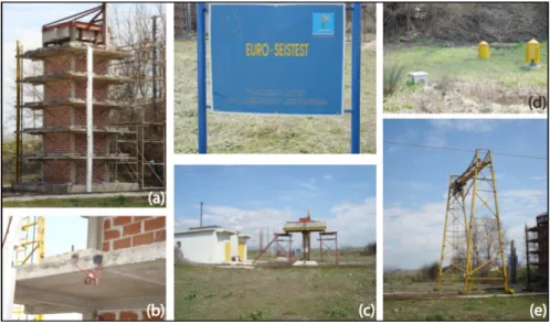
4.4 Test site of EURO-SEISTEST on Stivos, Thessaloniki . . . 35
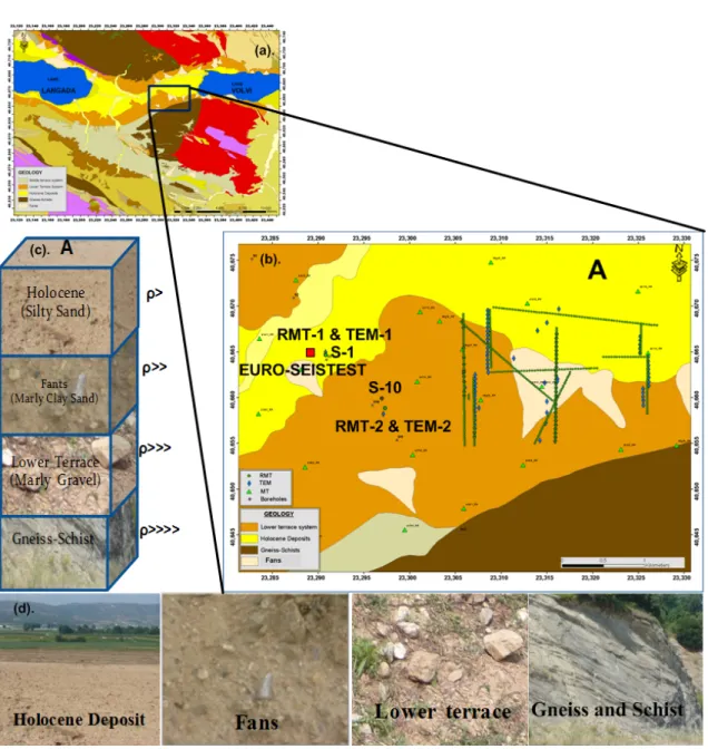
4.5 Regional geological map . . . 36
4.6 Stratigraphic coloumn of the Premydonian system . . . 38
4.7 Geological map and the geophysical profiles . . . 40
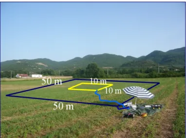
4.8 Panorama and topography of the study area . . . 41
4.9 The first and the second geophysical campaign . . . 42
4.10 The first and the second geophysical campaign of RMT and TEM data plotted on geological map . . . 43
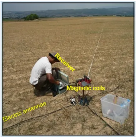
4.11 RMT field measurement using RMT-F system in the research area . . 45
4.12 Location of RMT measurements in the research area . . . 45
4.13 The azimuth of existing radio transmitters in the research area . . . . 46
4.14 Setup of TEM soundings performed using central loop (Tx: 50 m × 50 m and Rx:10 m × 10 m) configuration . . . 47
4.15 Location of TEM measurements in the research area . . . 47
4.16 Problem of Nano TEM data . . . 48
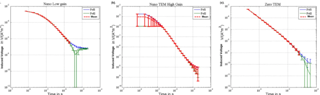
4.17 Current function and transient Nano TEM and Zero TEM . . . 49
4.18 Comparison between data using external damping and without ex- ternal damping of Nano TEM Modes . . . 49
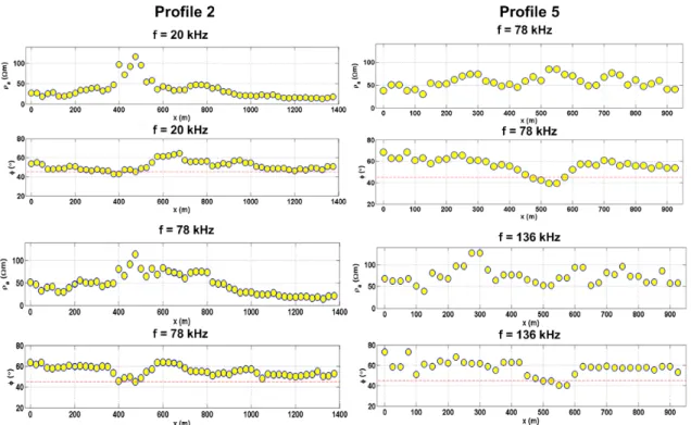
5.1 Raw data of RMT along profile 2 and profile 5 . . . 51
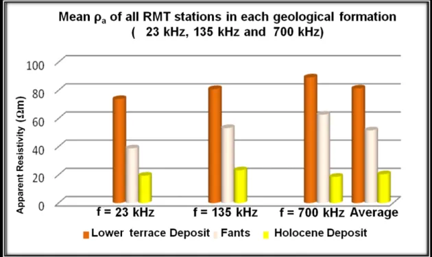
5.2 Average apparent resistivities for different geological formations . . . 52 vi
LIST OF FIGURES vii
5.3 TEM raw data of two polarities of each mode . . . 53
5.4 Deconvolution of TEM transient . . . 53
5.5 Combination of all three data deconvolution results of Nano TEM Low gain, Nano TEM high gain and Zero TEM . . . 54
5.6 1-D Occam inversion of RMT and TEM data . . . 57
5.7 1-D equivalence models for RMT data . . . 58
5.8 1-D equivalence models for TEM data . . . 59
5.9 Data fitting for RMT station 64 and TEM station 2 . . . 62
5.10 Correlation of RMS error with homogenous starting model using dif- ferent number of layers . . . 63
5.11 1-D Marquardt and Occam’s inversion models on RMT station 20 and TEM station 28 . . . 65
5.12 1-D Marquardt inversion models for RMT data . . . 66
5.13 1-D Marquardt inversion models for TEM data . . . 67
5.14 RMT and TEM data at reference site close to borehole S-1 . . . 68
5.15 Correlation of RMT and TEM data with borehole S-1 . . . 70
5.16 Correlation of RMT and TEM data with borehole S-10 . . . 70
5.17 1-D Marquardt model of RMT data on profile 2 . . . 72
5.18 1-D Marquardt model of TEM data on profile 2 . . . 74
5.19 1-D Marquardt model of TEM data on profile 3 . . . 74
5.20 Importance value distribution of RMT model along profile 2 . . . 75
5.21 Importance value distribution of TEM model along profile 3 . . . 75
5.22 RMS distribution of 1-D model on RMT and TEM data along profile 2 76 5.23 2-D conductivity model of profile 2 . . . 78
5.24 2-D conductivity model of profile 5 . . . 78
5.25 Fitting of measured and calculated data of 2-D RMT data for selected stations at profiles 2 and 5 . . . 80
5.26 Fitting of measured and calculated data of 2-D RMT data for selected frequencies at profiles 2 and 5 . . . 81
5.27 Correlation of 1-D and 2-D conductivity models of RMT data at profile 2 82 5.28 Improvement of geological map . . . 84
5.29 Correlation of 2-D models of RMT data with gological map . . . 85
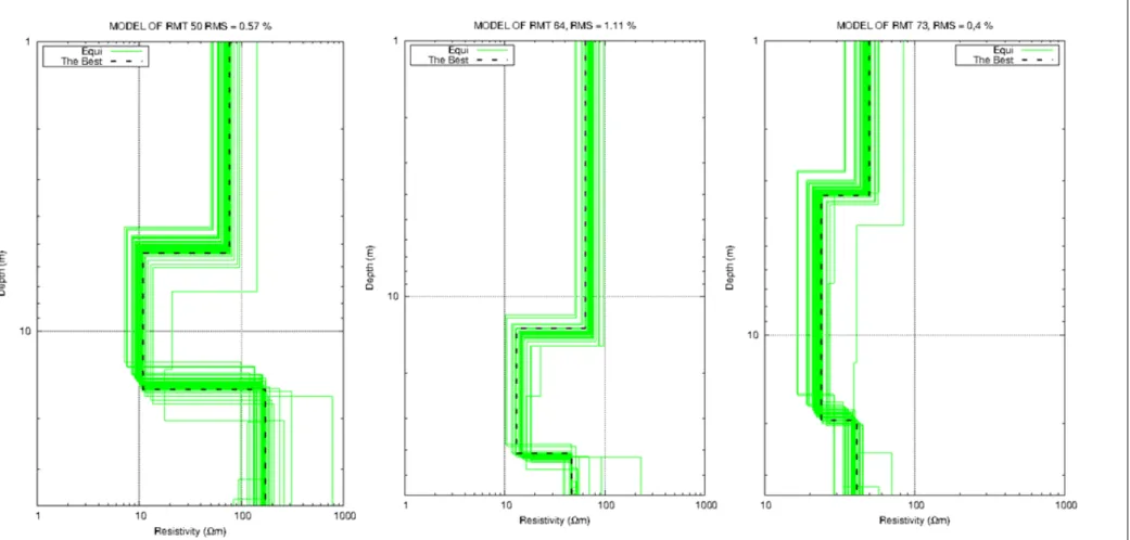
6.1 1-D model of sequential inversion at station 50 . . . 88
6.2 Sequential inversion at station 70 . . . 89
6.3 All 1-D conductivity models of sequential inversion along profile 2 . . 91
6.4 All RMS errors of sequential inversion at profile 2 . . . 92
6.5 Joint RMT 1 and TEM 1 inversion and correlation between with borehole S-1 . . . 94
6.6 1-D model of joint RMT and TEM inversion on profile 2 . . . 95
6.7 Importance values distribution of joint inversion along profile 2 . . . 96
6.8 1-D single RMT, TEM, sequential and joint models at station 58 . . 97
6.9 1-D of single RMT, TEM, sequential and joint inversion models on profile 2 . . . 99
7.1 Homogeneous model of 80 Ωm to test 3-D algorithm . . . 102
7.2 Testing 3-D forward modeling algorithm based on 2-D model . . . 103
viii LIST OF FIGURES
7.3 Comparison of 2-D and 3-D at frequency (f = 11kHz) and (f = 769
kHz) . . . 104
7.4 3-D forward modeling of profile 2 . . . 106
7.5 3-D forward modeling of the top layer . . . 107
7.6 3-D forward modeling of all RMT profiles . . . 109
7.7 Data analysis of 3-D forward modeling . . . 110
A.1 1-D conductivity model of RMT data on profile 1 . . . 121
A.2 1-D conductivity model of RMT data on profile 2 and 3 . . . 122
B.1 1-D conductivity model of TEM data on profile 1 in the first field campaign . . . 123
B.2 1-D conductivity model of TEM data in the first field campaign . . . 124
B.3 1-D conductivity models of TEM data on profile 1 . . . 125
B.4 1-D Occam’s models of TEM data on profiles 2 and 3. . . 126
C.1 1-D conductivity models of sequential inversion of All fix and All fix CF at profile 1 . . . 127
C.2 1-D conductivity models of sequential inversion of All free and All free CF at profile 1 . . . 128
C.3 1-D conductivity models of sequential inversion of All fix and All fix CF at profile 3 . . . 129
C.4 1-D conductivity models of sequential inversion of All free and All free CF at profile 3 . . . 130
D.1 1-D of sequential inversion model at profile 1 . . . 131
D.2 1-D of sequential inversion model at profile 2 . . . 132
D.3 1-D of sequential inversion model at profile 3 . . . 132
E.1 1-D conductivity model of joint RMT and TEM inversion at profiles 1 and 3 . . . 133
F.1 2-D conductivity models of RMT at profile 7 and profile 8 . . . 134
H.1 Three dimensional modeling . . . 138
H.2 Three dimensional responses of Zxy and Zyx . . . 139
List of Tables
2.1 Resistivity values for different materials . . . 7 2.2 Physical parameters and operators used for describing EM fields . . . 7 4.1 Historical earthquakes in Northern Greece since 500 A.D . . . 34 4.2 Parameter of RMT survey design in two field campaigns . . . 44 4.3 Parameter of TEM survey design in two field campaigns . . . 46 5.1 Penetration depth of RMT measurements on holocene deposit, fans
and lower terrace deposit. . . 55 5.2 Approximation of shallow penetration depth of TEM measurements
on holocene deposit, fans and lower terrace deposit. . . 56 5.3 Approximation of large penetration depth of TEM measurements on
holocenen deposit, fans and lower terrace deposit. . . 56 5.4 Starting model for Marquardt inversion of single RMT and single
TEM data . . . 60 5.5 Importance values for different inversion results of RMT data at sta-
tion 64 with different starting models . . . 64 5.6 Importance values of RMT and TEM at boreholes S-1 and S-10 . . . 69 5.7 Resistivity value distribution from correlation between boreholes and
geophysical data. . . 71 5.8 Analysis of fault structure based on importance parameter . . . 72 6.1 Models and importance parameters of single RMT, single TEM and
sequential inversion on station 50 . . . 87 6.2 Models and importance parameters of sequential inversion on station 54 90 6.3 Models and importance parameters of sequential inversion on station 58 90 6.4 Models and importance parameters of sequential inversion on station 70 91 6.5 Models and importance parameters of single RMT, TEM and joint
inversions at boreholes S-1 and S-10 . . . 93 6.6 Model and importance parameters of RMT, TEM and joint inversion
at station 56 . . . 95 6.7 Model and importance parameters of RMT, TEM and joint inversion
at station 58 . . . 96 6.8 Model and importance parameters of RMT, TEM and joint inversion
at station 64 . . . 96 6.9 1-D conductivity model of RMT, TEM, sequential and joint inversion
on profile 2 at depth 14-20 m . . . 98 ix
x LIST OF TABLES
6.10 1-D conductivity model of RMT, TEM, sequential and joint inversion
on profile 2 at depth 75-90 m . . . 98
J.1 GPS coordinates of RMT data of RMT 1 - RMT 30 . . . 144
J.2 GPS coordinatess of RMT data on profile 1 . . . 145
J.3 GPS coordinatess of RMT data on profile 2 . . . 146
J.4 GPS coordinatess of RMT data on profile 3 . . . 147
J.5 GPS coordinatess of RMT data on profile 4 . . . 148
J.6 GPS coordinatess of RMT data on profile 5 . . . 149
J.7 GPS coordinatess of RMT data on profile 6 . . . 150
J.8 GPS coordinatess of RMT data on profile 7 . . . 151
J.9 GPS coordinatess of RMT data on profile 8 . . . 152
K.1 GPS coordinates of TEM data on TEM 1 - TEM 30 and profile 1 . . 153
K.2 GPS coordinates of TEM data on profile 2 and profile 3 . . . 154
Abstract
The Volvi basin is an alluvial valley located 45 km northeast of the city of Thes- saloniki in Northern Greece. It is a neotectonic graben (6 km wide) structure with increasing seismic activity where the large 1978 Thessaloniki earthquake occurred.
The seismic response at the site is strongly influenced by local geological conditions.
Therefore, the European test site “EURO-SEISTEST” for studying site effects of seismically active areas is installed in the Volvi-Mygdonian Basin.
The ambient noise measurements from the east area of EURO-SEISTEST give strong implication for a complex 3-D tectonic setting. Hence, near surface Electromagnetic (EM) measurements are carried out to understand the location of the local active fault and the top of the basement structure of the research area. The Radiomag- netotelluric (RMT) and Transientelectromagnetic (TEM) measurements are carried out along eight profiles, which include 443 RMT and 107 TEM soundings.
The correlation between the borehole data and the interpreted TEM and RMT model generally shows six layers. The layers are identified as sedimentary and metamorphic rocks which in detail are: silty sand (10 - 30 Ωm), silty clay (10 - 30 Ωm), silty clay marly (30 – 50 Ωm), sandy clay (50 - 80 Ωm) and marly silty sand (> 80 Ωm) and basement (gneiss and schist) (> 80 Ωm) with varying thick- nesses.
To analyze the structure of the research area, interpretation of multidimensional models (1-D, 2-D, 3-D) is carried out. The 1-D model and the 2-D model derived from RMT data show a clear indication of the fault structure distribution in the research area. From the analysis, there can be found that the fault structure is associated with marly silty sand with a resistivity of more than 80 Ωm.
The correlation of the RMT 2-D model with the geological map provides a good fitting to the surface structure. Due to the high resistivity of the top layer, the skin depths of the RMT soundings are approximately 35 m. The TEM data gives a detailed description about the deeper structure down to the depth of 200 m. Joint and sequential inversions of RMT and TEM data can provide clear information from the surface to the deep structure. Single and joint inversions of RMT and TEM give a consistent result in which both identify the fault structure.
Three dimensional modeling of RMT data is implemented to provide a representa- tive model of all conductivity structures in the research area. The overall number of cells in the 3-D model is 2,317,000 cells (nx = 220 cells, ny = 220 cells and nz = 45 cells) modeling the research area with size of 2.4 km× 2.4 km. 3-D models provide a detailed description of the normal fault structure at depths of about 5 to
xi
xii LIST OF TABLES
25 m and thicknesses of 20 m. According to the analyses, a normal fault is located next to the EURO-SEISTEST site, with a strike direction of N 70◦ E.
Zusammenfassung
Das Volvi-Becken befindet sich in einem alluvialen Tal, das 45 km nord¨ostlich von Thessaloniki im Norden Griechenlands liegt. Es ist eine neotektonische Graben- struktur (von 6 km Breite) mit zunehmender seismischer Aktivit¨at, in der 1978 das relativ starke Thessaloniki-Erdbeben stattgefunden hat. Die seismische Response vor Ort ist stark beeinflußt von den lokalen geologischen Gegebenheiten. Deshalb wurde der europ¨aische Teststandort “EURO-SEISTEST” im Volvi-Mygdonischen Becken eingerichtet, um ortsabh¨angige Effekte von seismisch aktiven Gebieten zu untersuchen.
Die Messungen des Hintergrundrauschens aus dem Bereich ¨ostlich des EURO - SEIS- TEST - Gebietes weisen deutlich auf eine eine komplexe, 3-dimensionale, tektonische Struktur hin. Daher werden zur Erkundung der Schichtung oberhalb des Grundge- birges und der Lage der lokalen, aktiven Verwerfung oberfl¨achennahe Elektromag- netik Messungen (EM) durchgef¨uhrt. Radiomagnetotellurik (RMT) und Transien- telektromagnetik (TEM)-Messungen werden entlang von 8 Profilen durchgef¨uhrt, welche 443 RMT- und 107 TEM-Sondierungen beinhalten.
Die Korrelation zwischen den Bohrlochdaten und den interpretierten TEM- und RMT-Modellen zeigt im Allgemeinen einen 6-Schicht-Fall. Die Schichten werden identifiziert als sediment¨are und metamorphe Gesteine, im Einzelnen: schluffiger Sand (10 – 30 Ωm), schluffiger Lehm (10 – 30 Ωm), schluffiger lehmiger Mergel (30 – 50 Ωm), sandiger Lehm (50 – 80 Ωm) und mergeliger schluffiger Sand (>80 Ωm) und Grundgestein (Gneis und Schiefer) (> 80 Ωm) mit unterschiedlichen Schicht- dicken.
F¨ur die Analyse der Struktur des Untersuchungsgebietes wird die Interpretation von mehrdimensionalen Modellen (1-D, 2-D, 3-D) durchgef¨uhrt. Die 1-D- und 2- D-Modelle, die aus den RMT-Daten stammen, zeigen deutliche Auswirkungen des Verlaufs der Verwerfungen im Untersuchungsgebiet. Und aus dieser Analyse kann man erkennen, daß die Verwerfungsstruktur mit mergeliger schluffiger Sand eines spezifischen Widerstandes von mehr als 80 Ωm verbunden ist.
Die Korrelation des 2-dimensionalen RMT-Modells mit der geologischen Karte liefert eine gute Anpassung an die oberfl¨achennahe Struktur. Wegen des hohen spezifischen Widerstandes der obersten Schicht liegen die Skintiefen der RMT-Sondierungen etwa bei 35 m. Die TEM-Daten ergeben eine detaillierte Beschreibung der tieferen Struk- tur bis hinunter zu einer Tiefe von 200 m. Gemeinsame und sequentielle Inversion von RMT- und TEM-Daten liefern eindeutige Informationen von der oberfl¨achenna- hen bis zur tiefen Struktur. Die Einzelinversionen und die gemeinsame Inversionen
xiii
xiv LIST OF TABLES
von RMT und TEM ergeben einen konsistenten Befund nach welchem beide die Verwerfung identifizieren.
Dreidimensionale Modellierung der RMT-Daten wird ausgef¨uhrt, um ein repr¨asenta- tives Modell f¨ur alle Leitf¨ahigkeitsstrukturen im Messgebiet zu erhalten. Die Gesam- tanzahl der Zellen des 3-D-Vorw¨artsmodells ist 2.317.000 Zellen (nx = 220 Zellen, ny = 220 Zellen und nz = 45 Zellen), die das Meßgebiet mit einer Ausdehnung von 2,4 km × 2,4 km modellieren. Die 3-D-Modelle liefern eine genaue Beschreibung der Struktur der senkrechten Verwerfung in einer Tiefe von etwa 5 – 25 m bzw. mit einer M¨achtigkeit von 25 m. Entsprechend der Analysen befindet sich neben dem EURO-SEISTEST-Gebiet eine senkrechte Verwerfung mit einer Streichrichtung von N 70◦ O.
Chapter 1 Introduction
It is well known that earthquake generally produces several damages. Moreover if it occurs near densely populated area, it is required additional efforts to provide the detailed knowledge on active faulting, shear wave velocities and its correlation with seismicity in the concerned area. Faults are not usually isolated structures mechanically, however they exist within a population of faults and they may inter- act with each other through their stress fields. Destructive resulting from the large earthquake amplification effect has been widely reported during recent years, such as the case of Izmit and Duzce earthquake in 1999 [Hubert-Ferrari et al., 2001], Aceh, North Sumatra earthquake in Indonesia [Ghobarah et al., 2006] and Pacific coast in Japan in 2011 [Takahashi et al., 2012]. Prior to an earthquake hazard, it is important to evaluate the behavior of earthquake faults, the expected objective being the assessment of the future seismic hazard.
Northern Greece is an area with one of the most seismically active region in Europe.
Several earthquakes occurred during 20th century. The largest earthquake in recent time with magnitude of 6.5 happened in June 1978. The epicenter1 was located between lakes of Volvi and Langada near Thessaloniki, Northern Greece [Papaza- chos et al., 1979]. The area was characterized through a neotectonic graben (5.5 km wide) structure associated with an active fault structure, elongated in NNW-SSE direction of the mentioned lakes [Raptakis et al., 2002]. Hence, the “Euroseistest Volvi-Thessaloniki” project, a strong-motion test site (Euroseistest) for Engineering Seismology was put at the location of the epicentre. The main purpose of Euroseis- test was to provide high quality geophysical data due to earthquake recordings that allows studying soil-building interactions.
This presented work refers to Volvi basin located in the Mygdonian graben, ca.
45 km of northeast Thessaloniki city. Since the Volvi basin area was affected by earthquake in 1978, various types of geophysical surveys have been conducted with an intensive research. In the past, seismotectonic studies were implemented by var- ious researchers in this area [Papazachos et al., 1979, Soufleris and Stewart, 1981, Mercier et al., 1983]. These studies aim to investigate the focal mechanism of fault structure, which was responsible for Thessaloniki earthquake in 1978. The main strike of faults in the area which produced major shock of the recent seismic se-
140.7◦N , 23.3◦E, depth = 16 km
1
2
quence was found along the Villages Stivos- Scholari - Evangelismos with a dip of N85◦E [Papazachos et al., 1979]. The earthquake sequence is a complicated pattern and having irregular direction. The complicated fault patterns are including NW- SE, NE-SW, E-W and NNE-SSW- trending faults, which are associated with active seismic [Soufleris and Stewart, 1981,Pavlides et al., 1990,Tranos et al., 2003]. Based on numerical modeling using seismic waves, geological structure in Volvi basin has been constructed with 2-D and 3-D models [Semblat et al., 2005, Manakou et al., 2010]. These models give information about site effects assessment which corre- sponds to ground motion distribution in Volvi Basin.
Several non-seismic geophysical studies have also been implemented in the Mygdo- nian Basin. Gravity and aeromagnetic surveys [Thanassoulas, 1983] aim to study the deeper structure of the area. These surveys show the existence of a tectonic horst in the basement of Langada valley. In the project, “Euroseistest Volvi-Thessaloniki”, MT and gravity studies were carried out in the Volvi Basin in order to define the geological structure of the basin [Savvaidis et al., 2000, Makris et al., 2002]. These results proposed that the basement corresponds to gneiss and schist with rock re- sistivities larger than 80 Ωm. The top of the basement was located at a depth of around 200 m. Savvaidis et al. [2000] and Makris et al. [2002] analyzed that the magnetotelluric strike that can be associated with the normal fault strike has a di- rection of N65◦E. The combination of electromagnetic methods such as Controlled Source Audio Magnetotelluric (CSAMT) and Very Low Frequency (VLF) was used to study tufa outcrops in the Mygdonian Basin [Gurk et al., 2007].
Previous CSRMT (Controlled Source Radiomagnetotelluric) measurements for the investigation of the fault structure in the northwest Euroseistest was carried out by Bastani et al (2011). The CSRMT system uses two frequency bands, a CSAMT band with a frequency range from 1 kHz – 10 kHz and a RMT band (without controled source) in a frequency range from 10 - 250 kHz. Bastani et al. [2011] proposed that the faults in this area have direction of NE-SW to E-W. Their result provided an image of resistivity variation from surface down to a depth about 100 m. Borehole data showed the depth to the bedrock up to 132 m. Due to limitation of the Lower frequency in this method, the top of basement was not resolved towards the centre of the basin. However, detailed information of the fault structure in the northeast of their research area has not been verified so far.
The ambient noise measurements from the east area of Euroseistest experiment give strong implication for a complex 3-D tectonic setting. This corresponds to local ge- ological structure in the study area. Geological information denotes that the study area consists of four major units [Jongmans et al., 1988]: holocene deposit, fans, lower terrace deposit and the basement of Mygdonian basin composing gneiss and schist, located around 180 meter depth [Jongmans et al., 1988, Savvaidis et al., 2000,Raptakis et al., 2002]. Based on conductivity contrast of these layers and the location of the basement, we carried out a research using shallow (0 - 200 m) EM surveys using RMT and TEM methods. In order to understand the distribution of the active fault and the top of basement structure in northeast EURO-SEISTEST, these surveys were conducted.
3
The RMT is a relatively new electromagnetic technique of applied geophysics and it is an extension of VLF method to higher frequencies. M¨uller and his group at Neuchˆatel pioneered the RMT technique in its original and scalar form [Stiefelhagen and M¨uller, 1997,Turberg et al., 1994]. It was applied in hydrogeological application in Switzerland. The combination of RMT (14 - 250 kHz) and CSAMT (1 - 12 kHz) measurements for groundwater exploration in an area in Sweden was implemented byPedersen et al. [2005].
One of the RMT devices in environmental application was developed byTezkan and Saraev[2008],Tezkan[1999],Tezkan et al.[2000],Tezkan[2009] and his group at the University of Cologne, Germany. This RMT was based on tensor form, but so far the data was realized as scalar. The RMT technique is one of ground based geophysical methods and is faster than the other ground based geophysical methods. In this method, a huge amount of data can be readily acquired, which corresponds to the frequencies of available radio transmitters. Now the RMT method is more effective in Europe, where transmitters in the necessary frequency range are common.
The RMT technique has been successfully applied for different purposes, mainly in environmental prospecting, such as groundwater exploration [Pedersen et al., 2005, Tezkan, 2009] and waste disposal [Zacher et al., 1996, Tezkan et al., 2000]. The application of RMT method is applied for investigation of fracture zone [Linde and Pedersen, 2004].
TEM method has gained popularity over the past century and it is an inductive method. TEM is good for mapping the depth of and the extent of conductors, but is relatively less sensitive at distinguished conductivity contrast in low conductivity range [Pellerin and Wannamaker, 2005]. In the past, the TEM method was applied for groundwater exploration [McNeill, 1990, Spies and Frischknecht, 1991, Sørensen et al., 2004]. Recently, the TEM technique has been successfully applied for the measurements of near surface electrical anisotropy in fault zone central North-West Victoria [Dennis and Cull, 2012].
The penetration depth of TEM method refers to the depth associated with the distribution of conductivities. The surface conductivity distribution is related to early transient, the deeper structure is corresponding to late time of TEM sound- ing. The TEM data are sensitive to vertical inhomogeneities, but less affected by lateral inhomogeneities [Helwig, 1994]. In order to investigate shallow penetration, a combination of TEM and RMT is recommended.
This dissertation uses a combination of RMT and TEM methods, in order to get overall description of the fault structures in the study area. The joint inversion algorithm for magnetotelluric and direct current was introduced byVozoff and Jupp [1975]. The application of 1-D joint inversion an EM methods (MT and TEM) was used byMeju [1996]. Harinarayana [1999] provided a summary on the combination of electrical and electromagnetic techniques. Combining data from two different methods of RMT and TEM is beneficial because they are complementary. The RMT data give information about the top layers, whereas the deeper structures can be resolved by TEM data. Combining TEM and RMT inversion was successfully applied on geological and engineering problems in the past [Tezkan et al., 1996,
4 1.1. SCOPE OF PRESENTED THESIS
Schwinn, 1999, Steuer, 2002, Farag, 2005].
Joint inversion can increase the number of important model parameters and it can also decrease the ambiguity of the model [Vozoff and Jupp, 1975]. Hence, the joint inversion of RMT and TEM data will produce good resolution of model parameters in shallow and deeper parts of fault structure.
Finally, the application of near-surface electromagnetic methods, RMT and TEM, are promising methods to derive geological structure and the top of basement in the graben structure of the Volvi basin. The correlation between a priori informa- tion (boreholes data) and the conductivity models of 1-D and 2-D provides accurate interpretation of local geological structure in the study area. The representative con- ductivity model of structure in the research area can be performed by 3-D forward modeling of RMT data to obtain clear description of fault structure.
1.1 Scope of Presented Thesis
The objective of the presented study is to investigate local geological structure and the top of the basement of the Volvi Basin, Northern Greece. The geophysical surveys are carried out using electromagnetic methods (RMT and TEM ). The in- vestigations are limited to near surface studies with shallow depth (< 200 m). It is expected that the complex geological structure and the vertical distribution of resistivity layers can be defined by RMT and TEM methods.
DIKTI (Directorate General of Higher Education of Indonesia) scholarship financed me to pursue during my PhD studies at University of Cologne, Germany. The field campaign was supported by Marie Curie project: IGSEA – Integrated Neoseismic Geophysichal Studies to Asses the Site Effect of the EURO-SEISTEST Area in Northern Greece-PERG03-GA-2008-230915.
The entire work is presented systematically in the form of the following eight chap- ters. The brief descriptions of these are mentioned below:
Chapter - 2 describes the conceptual background of RMT and TEM methods.
Chapter - 3 deals with the theory of EM data inversion.
Chapter - 4 consists of geology and EM field campaign. Geological problem of unclear local active fault structure in the Volvi Basin is mentioned. For this pur- pose, the RMT and TEM measurements are performed at various geological units in the research area. RMT surveys are carried out along eight profiles with distances among stations of 25 m. The total length is around 12 km with total of 443 RMT soundings. The TEM data is spread along three profiles with distances among sta- tions of 50 m. The overall 107 soundings are obtained from TEM data. The problem of geophysical measurements in the research area also describes in this chapter.
Chapter - 5comprises results and interpretations of single inversions of RMT and TEM data. The RMT and TEM data quality are shown in this chapter. In order to calibrate the geophysical data, boreholes data as priori information have been correlated. Two schemes are used to analyze the fault structure: the importance value of model parameters and geological point of view. The clear existence of fault
1.1. SCOPE OF PRESENTED THESIS 5
structure in the Volvi basin can be seen cleary in single 1-D and 2-D models of RMT data. The correlation between all 2-D conductivities of RMT models and the geological map identifies that the research area has a normal fault structure with direction of N70◦ E.
Chapter - 6, the joint and sequential inversion of RMT and TEM data is realized.
The sequential inversion uses resistivity of first layer ρ1, second layer ρ2 and thick- ness h1 of RMT models, as priori models for the inversion process of TEM data.
These inversions are implemented with four approches: all fixed parameters (ρ1, ρ2 and h1 ) with either fixed or free Calibration Factor (CF) and other two approches using free parameters with either free and fixed CF. The result of joint inversion was in agreement with assumption as the RMT data are resolved the surface layer at depth down to 40 m, and TEM data is small enough to resolve the surface struc- ture (z < 10 m), however it can resolve the deeper structure down to 200 m of depth, depending on the resistivity structure. The joint and sequential models can both represent 1-D single inversion of RMT and TEM data. The model parameters are well resolved in joint inversion in comparison with the single RMT and TEM inversions. Joint and sequential inversions have proven to be able to replace the information on the shallow depths missing from the TEM data due to a technical problem of Nano TEM data .
Chapter - 7 discusses how 3-D forward modeling is created on RMT data. The verification 3-D model with homogenous half space and 2-D models also performed in this chapter. The 3-D forward modeling of RMT data provide a representative model of all conductivity structures in the research area.
Finally the major findings of this dissertation are summarized and concluded. Sug- gestions for the future work in the area are also given in Chapter - 8.
Chapter 2
Basic Electromagnetic Theory
This chapter presents the two electromagnetic methods, namely Radiomagnetotal- luric and Transientelectromagnetic. The principle of RMT and TEM are discussed, i.e. data acquisition, processing and interpretation. In the EM methods, the sub- surface electrical resistivity is essential due to the penetration depth of the EM fields.
2.1 Archie’s Law
The resistivity of water bearing rocks or soil depends on the salinity of water, poros- ity and saturation. The electrical conductivity of the sediment is essentially influ- enced by porosity, permeability and the amount of water content. The relationship between the resistivity and the porosity of the matrix in a sedimentary rock is given by the empirical formula of Archie[1942]:
ρ0 =ρw ×a×S−nϕ−m (2.1)
where ρ0 is bulk resistivity (Ωm), ρw = resistivity of the pore fluid (Ωm), a = proportional factor (0.5<a <1), S = saturation (0 <S ≤1 ), n = saturation ex- ponent (n≈2), ϕ = effective porosity (0< ϕ ≤1) and m = cementation exponent (1.3 < m < 2.5 ). A classification of resistivity ranges for different rock types and fluids types can be seen in Table 2.1.
The EM geophysical methods commonly provide information about the earth’s con- ductivity distribution. The elementary laws of EM fields are governed by Maxwell’s equations. The physical earth parameters determining the response are the electri- cal resistivity (ρ), the magnetic permeability (µ) and the electric permittivity ().
The parameters commonly used for describing EM fields and there S I units are listed in Table 2.2. A detailed information of geophysical EM methods are given in Nabighian[1979] and Ward and Hohmann [1988].
6
2.1. ARCHIE’S LAW 7
Table 2.1: Resistivity values for different materials [Palacky, 1988]
Material Resistivity [Ωm]
Massive sulphides 0.01 - 1
Salt water 0.1 - 1
Fresh water 3 - 100
Clays 3 - 100
Shales 3 - 50
Sandstone 50 - 1000
Igneous and Metamorphic 103−105
Table 2.2: Physical parameters and operators used for describing EM fields
Symbol Property SI unit
E~ electric field intensity Vm
D~ electric flux density mAs2
B~ magnetic flux density Tesla = mVs2
H~ magnetic field intensity Am
~j current density mA2
q electric charge mAs3
0= 8.854· 10−12 permittivity of free space VmAs
r dielectric constant non-unit
= 0r electrical permittivity Asm µ0 = 4π · 10−7 permeability of free space AmVs
µr relative permeability non-unit
µ=µ0µr magnetic permeability AmVs
σ electric conductivity mS = VmA
ρ resistivity Ωm = VmA
f frequency Hz = 1s
ω=2πf angular frequency 1s
I current A
k wavenumber non-unit
c0 = õ1
0ε0 = 3·108 EM wave velocity in vacuum ms
∇=(∂x∂ ,∂y∂ ,∂z∂ ) Del operator non-unit
∇2= (∂x∂22,∂y∂22,∂z∂22) Laplace operator non-unit
8 2.2. MAXWELL’S EQUATIONS
2.2 Maxwell’s Equations
Maxwell equations1 describe the principle of the properties of all EM fields and can be written as:
∇ ·D~ =q (2.2)
∇ ·B~ = 0 (2.3)
∇ ×E~ =−∂ ~B
∂t (2.4)
∇ ×H~ =~j+∂ ~D
∂t (2.5)
The interaction between matter and field is described by the material equation. The current density which flows in a material medium as the result of the electric field density according to Ohm’s Law is:
~j=σ ~E (2.6)
The relation between the respective electric and magnetic fields in the material is defined by
D~ =ε ~E =ε0εrE~ (2.7)
B~ =µ ~H =µ0µrH~ (2.8)
2.2.1 Telegraph and Helmholtz Equations
From Faraday’s (equation 2.4) and Ampere’s laws (equation 2.5) by using the vector identity:
∇ ×(∇ ×A) =~ ∇(∇ ·A)~ − ∇2A~ (2.9) whereA~is an arbitrary vector field withA~ ∈R3, we get theTelegraph equations:
∇2E~ =σµ∂ ~E
∂t +εµ∂2E~
∂t2 (2.10)
∇2H~ =σµ∂ ~H
∂t +εµ∂2H~
∂t2 (2.11)
with F~ ∈ {E,~ H}~ we can simplify:
∇2F~ =σµ∂ ~F
∂t +εµ∂2F~
∂t2 (2.12)
1The equation is found by JAMES CLERK MAXWELL (1864-1879)
2.2. MAXWELL’S EQUATIONS 9
Without losing generality, we can assume the time variation of the fields is in a simple harmonic form (solution of the Telegraph’s Equation):
F~ =F~0e−iωt (2.13)
whereF~0 is amplitude ofF~.
From solving equation 2.12 with equation 2.13, we have Helmholtz’s Equation:
∇2F~ =−k2F~ (2.14)
with :
k2 =εµω2(1 + σ
ωεi) (2.15)
F k~ 2 = F εµω~ 2
| {z }
displacement current
− F iσωµε~
| {z }
conduction current
(2.16) k is the complex wave number. The first term (εµω2) and second term (iσωµε) on the right hand of equation 2.16 are related to the displacement current and the conduction current respectively.
2.2.2 Quasi-static approximation
From equation 2.16, we can derive the relationship beetwen conduction current and displacement current. If the conduction current is much larger than the displace- ment current, we have the quasi static approximation:
ωµσ ω2µε = σ
ωε 1 (2.17)
when the angular wave numberk1, the Helmoholtz equation is essentialy repre- sent a diffusion equation. For average resistivity2of≈80 Ωm with highest frequency of f =1 MHz, we get:
σ
ωε = 1
ρωε = 1
80×6.3·106×8.85·10−12 = 224.11 (2.18) The calculation of the quasi-static approximation in formula 2.18 shows that the displacement currents for RMT frequencies (10 kHz - 1 MHz) can be neglected in the study area. However displacement currents should be considered when the investigation area has very high resistivity [Persson and Pedersen, 2002].
2The avarege resistivity distribution in the study area
10 2.3. ELECTROMAGNETIC METHODS
2.3 Electromagnetic Methods
EM methods are powerful tools in environmental and geological investigations. Sav- eral techniques of EM have been developed in many applications, such as mining, geothermal, hydrogeological investigations, etc. To determine subsurface electrical resistivity, the EM methods use the principle of electromagnetic induction. A pri- mary EM field induces electric and magnetic fields in the subsurface. There are generally two kind of sources: natural or artificial. The EM field is diffusive when the applied frequency is low, i.e the MT approximation is valid. The classification therefore also depends on the subsurface resistivity. Active source methods can be implemented in both the frequency domain and time domain mode.
Frequency domain electromagnetic (FDEM) surveys begins with the injection of a time varying current into a transmitter coil. The time varying current gener- ates a magnetic field which induces a current in accordance with Faraday’s law.
The induced currents occur throughout the subsurface. These currents usually flow through the conductor in planes perpendicular to magnetic field lines from the trans- mitter. A secondary magnetic field is also generated from these induced currents.
The magnetic field lines of the secondary magnetic field are opposite to the induced currents. As these currents occur in the subsurface, the magnitude and distribution depend on transmitter frequency, power, geometry and the distribution of the elec- trical resistivity of the subsurface [Kaufman and Keller, 1983].
There are several FDEM methods usually applied which use a frequency dependent active source: Control Source EM (CSEM), Helicopter EM (HEM), Slingram. Other FDEM methods use plane waves as the source for EM induction in the ground, i.e., EM-waves generated by radio-transmitter or generated naturally by interaction of the solar wind with the magnethosphere or lighting. The examples for these methods are: MT [Cagniard, 1953, Tikhonov, 1950], Audiomagnetotellruic (AMT), CSAMT, Audio Frequency Magnetics (AFMAG), VLF and VLF resistivity mode (VLF-R) and RMT.
The magnitude of the secondary field is very small compared to the primary field. In this case, the measurement of the secondary magnetic field is the main problem for the controlled source EM method. To avoid this problem, time domain EM methods can be applied.
Time domain electromagnetic (TDEM or TEM) methods inject EM energy with a transmitter into the ground as transient pulses instead of continuous waves. Two types of transmitters are commonly used in TEM measurements: A loop source which forms a vertical magnetic dipole with inductive coupling to the ground and a grounded wire which forms a horizontal electric dipole with both inductive and galvanic coupling [Scholl, 2005]. There are two types of TEM methods based on the depth of the exploration; SHOTEM (Short Offset TEM) and LOTEM (Long- Offset TEM). In the SHOTEM, the diffusion depth is greater than the transmitter and receiver separation while in LOTEM (Long-Offset TEM), the diffusion depth is equal to or less than the receiver offset. The transmitter configuration is a grounded dipole in LOTEM [Strack, 1992].
2.3. ELECTROMAGNETIC METHODS 11
The Skin Depth
The amplitude of the secondary field generated in the ground is attenuated with depth. The primary magnetic field in TEM does not exist during measurement of the secondary magnetic field and this is one major advantage of TEM surveys over FDEM surveys. The absence of a primary field during TEM measurements enables the receiver loop to be put within the transmitter.
In EM methods, the terms “depth of penetration” and “skin depth” are often as- sumed to be synonymous. The skin depth is defined as the depth in which the field amplitude is attenuated by 1/e or approximately 37% of its value at the surface.
The skin depth is largely used as rough estimation of the investigation depth of the EM systems [Spies, 1989]. The skin depth in frequency domain (δF D) is given by
δF D = r 2
ωµσ ≈503 rρ
f (2.19)
Equation 2.19 is only an exact estimation for the homogeneous half space.
The RMT and TEM methods have greater penetration depth when the conductivity of the subsurface is lower. For exploring deep structures, late recording times and low frequencies are needed, respectively. In case of TEM surveys, the time-domain diffusion depths (δT D) at any time t is defined as:
δT D = r2t
µσ (2.20)
The depth of investigation is defined as the maximum depth in which a given target can be detected in a given host. The practical depth of investigation can be several skin depths in an ideal geological environment, whereas when it is in a complex or noisy geological area and for certain EM sounding systems, the depth of investi- gation can be much less than one skin depth. It is an empirical quantity and is influenced by the target properties and host medium as well as factors in regard to the investigation modality such as data processing and interpretation methods, sensor sensitivity, accuracy, frequency, coil configuration and ambient noise [Huang, 2005].
12 2.3. ELECTROMAGNETIC METHODS
2.3.1 Radiomagnetotelluric Method
The RMT method uses distant radio-transmitters in the frequency band (10 kHz - 1 MHz) as EM source-fields. The principle of this method is demonstrated schemat- ically in Figure 2.1. The EM fields can be assumed as plane waves. A radiated EM wave consists of coupled alternating vertical electrical and concentric horizontal magnetic fields, perpendicular to each other. The electromagnetic waves radiated from these transmitters diffuse into the conductive earth where they induce electric current systems. The magnetic field can be measured for selected frequencies with a coil and the electric field with two grounded electrodes.
Figure 2.1: Schematic diagram of RMT setup.
The skin depth of electromagnetic waves can be calculated for different frequen- cies according to equation 2.19. Figure 2.1 indicates that the highest frequency (f1) carries information of the shallow structure and the lowest frequency (f3) represents the deeper structure.
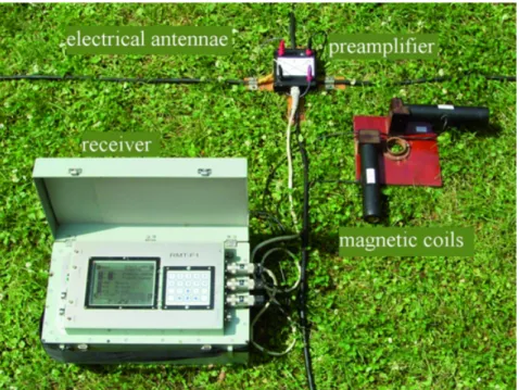
The RMT device utilized here is called RMT-F (Figure 2.2). The equipment uti- lized uses an extended frequency range from 10 kHz up to 1 MHz. The device has 4-channel recording (Hx, Hy, Ex, Ey) and was developed by the University of Cologne, Germany in cooperation with Microcor and University of St.Petersburg [Tezkan and Saraev, 2008] and [Microkor and St. Petersburg University, 2005]. The RMT-F system consists of two capacitive grounded electric antennas to measure electric fields, two magnetic coils to observe the magnetic field.
2.3. ELECTROMAGNETIC METHODS 13
Figure 2.2: RMT-F system from University of Cologne: Digital 4-channels receiver, electric antennae, magnetic coils and E-field preamplifier.
A concept about definition of electrical scalar impedance was developed from lay- ered medium usage to more complex geological environment by introducing the impedance tensor [Sims et al., 1971, Cagniard, 1953]. They have given a linear relationship between the horizontal components of the electromagnetic field at the surface of the earth as:
Ex =ZxxHx+ZxyHy (2.21)
Ey =ZyxHx+ZyyHy (2.22)
The above equation (2.21 and 2.22) can be written as matrix:
Ex
Ey
=
Zxx Zxy
Zyx Zyy
| {z }
Z
Hx
Hy
The complex quantitiesZxx, Zxy, Zyx, Zyy are the components of the impedance ten- sor. The components of impedance tensors have a function as electrical properties, orientation of sensors and direction of primary field.
14 2.3. ELECTROMAGNETIC METHODS
Apparent resistivitiesρaij and impedance phaseφaij [◦] can be derived from complex impedance, Z, using the formula of Cagniard [1953]:
ρaij = 1
ωµ|Zij|2 (2.23)
φij = tan−1[=(Zij)
<(Zij)] (2.24) where i, j ∈ {x, y} and i 6= j:
In a homogenous earth, the apparent resistivity equals to the time resistivity and the phase is π4 (45◦). But in 1-D layered earth surface, the phase decreases when EM field penetrates from higher conducting layer into lower conducting zone and reversely, it will increase when it penetrates from the lower conducting zone into the higher one.
Impedance tensor components are used as diagnostic tool to determine the dimen- sionality of subsurface structure seen from the intrinsic characteristics.
1. For 1-D resistivity distribution in the earth (layered model), the amplitude of impedance tensor elements are equal and the diagonal elements are zero. The impedance tensor reduces to a scalar impedance
Zxy =−Zyx, Zxx =Zyy = 0 (2.25) 2. If a 2-D resistivity structure represents the subsurface, of which the electric field is measured parallel or perpendicular to the strike direction, the compo- nents of impedance tensor are:
Zxy 6=Zyx, Zxx =Zyy = 0 (2.26) In the optimal 2D case, Maxwell’s equations are divided into two modes of polarization: transverse electric or TE mode, in which electric field is along the strike, and transverse magnetic or TM mode, having magnetic field along the strike direction.
3. In the 3-D case, all components of the impedance tensor are non-zero. The impedance skew is used as another indicator of dimensionality of the subsurface structure. It is introduced by Swift [1967] and he described skew as
S = |Zxx+Zyy|
|Zxy−Zyx| (2.27)
In 1-D (for noise free data), and in 2-D case when the x or y is along strike, skew is zero, while in 3-D case, it is not zero [Vozoff, 1987]. However, due to the limited number of radio transmitters in the field, not all impedace tensor components are available and thus, the skewness could not be calculated in the present thesis.
2.3. ELECTROMAGNETIC METHODS 15
2.3.2 Central Loop Transient Electromagnetic
The TEM method is an effective tool for investigating vertical changes in the earth.
By performing groundbased measurements, it is possible to cover large areas with this method. The most used field setup is the central loop or in-loop configuration.
For this setup, the receiver loop (Rx) is placed in the center of the transmitter loop (Tx) (Figure 2.3).
Figure 2.3: Diagram of central loop (in loop) TEM.
The basic principle of central loop TEM can be described with Figure 2.4 and Figure 2.5. Figure 2.4a shows the fundamental waveform used for central loop TEM.
The current in the transmitter loop produces a primary magnetic field. When the current flowing in the transmitter is turned off abruptly, the primary field induces eddy currents in the conductive underground corresponding to Maxwell’s equations.
This eddy currents produce a secondary magnetic field of which the propagation depending on the conductivity distribution in the subsurface. After current turn-off the time derivative of the secondary magnetic field is measured in the receiver loop at distinct the time points. The decay curve is a transient (Figure 2.4b).
Figure 2.4: Fundamental waveform for central loop TEM. (a) Current in the transmitter loop. (b) Secondary magnetic field measured in the receiver coil (modified after McNeill and Labson [1990]).
16 2.3. ELECTROMAGNETIC METHODS
Figure 2.5: Equivalent current filament concept in understanding the behavior of TEM fields over conducting half-space (after [Nabighian, 1979]).
Conducting Half-Space
In a conducting half space, the smoke ring effect of induced current can be approxi- mated with an equivalent current filament moving down at a velocityv = πσµt2 and with radiusa = 4.37tσµ [Nabighian, 1979].
Figure 2.5 shows that the maximum of the actual induced currents are moving down at an angle of 30◦, whereas the equivalent current filament moves downward at around 47◦. For central loop measurements, the analytic solution for the vertical magnetic fieldHz at the surface of a homogeneous half space can be found inWard and Hohmann[1988] as:
∂Hz
∂t =− Iρ
µ0σa3[3erf(θa)− 2
√πθa(3 + 2θ2a2)e−θ2a2] (2.28) where I is the transmitter current, θ = (ρµ4t)12, a is the transmitter-loop radius [m]
and erf(x) is the error function given by erf(x) = 2
π Z x
0
e−t2dt (2.29)
There are two common transformations from induced voltage to apparent resistivity.
The approximation for early and late time apparent resistivity can be derived from equation 2.28.
For early time (t →0), it gives:
∂Hzet
∂t =− 3I
µ0σa3 (2.30)
The apparent resistivity for early time is ρeta =−µ0a3
3I
∂Hz
∂t (2.31)
For late time (t→ ∞) the relevant asympotic formula can be given as:
∂Hzlt
∂t =− Ia2 20√
π(σµ0)32t−52 (2.32)
2.3. ELECTROMAGNETIC METHODS 17
The apparent resistivity for late time is ρlta = I23µ0a43
2023π13t53(−∂Hz
∂t )−23 (2.33)
The time behavior of the receiver coil output voltage at early time is constant, whereas at late time, it is proportional to t−52. For the vertical magnetic field, the early time is proportional toρ. Both, the early and late time approximation give a rough impression of the subsurface structure.
Nano TEM and Zero TEM
The investigation of shallow and deeper structures is effectively applied using Nano (Very fast turn-off) and Zero (slow-turn-off) TEM modes. The devices used are the NT-20 transmitter and GDP-32 II str (Figure 2.6)[Zonge Engineering and Research Organisation Inc., 2001].
This allows to measure TEM data in two distinct modes, according to different investigation depths. The devices can be synchronized, therefore the recording is performed in appropriate time frames. More information about two combinations between Nano and Zero TEM can be found in the manual by Zonge Engineering and Research Organisation Inc. [2001]. NanoTEM and ZeroTEM have been suc- cessfully applied in several areas for geomorphological and hydrogeological studies [Koch et al., 2003, Mollidor, 2008] and [Papen, 2011].
Figure 2.6: NT-20 transmitter (left) and GDP32 II receiver (right).
The injected currents in Nano and Zero TEM depend on the loop size and the location of the target. Nano TEM uses currents up to 3 A. The receiver records from 0.3 µs - 2.5 ms. In order to get information in the deeper structure, the Zero TEM mode can measure in a time window from 31µs - 6 ms. It is using relatively high current (about 10 A) and 50 - 55µs turn-off ramp time. Therefore, a combina- tion between Nano and Zero TEM can give information of the subsurface structures from shallow to great depth, depending on the conductivity distribution.
18 2.3. ELECTROMAGNETIC METHODS
Influece of Current Function
Prior to use Nano and Zero TEM modes with different ramp times, it is essential to know the behavior of the transient decay. In fact, the current function I(t) during turn off is considered as a linear ramp (see Figure 2.7).
Figure 2.7: Shutdown function with a ramptime of t0.
The relation of a linear current turn-off fuc- tion I0(t) with turn-off time t and induced voltageV0(t) is described byFitterman and Anderson [1987]. The measured voltage V0(t) can be described by a convolution in- tegral of the current-turn off function I0(t) and the uninfluenced earth responseV(t).
V0(t) = Z t
−∞
−dI0(t0)
dt0 V(t−t0) dt0 (2.34)
= 1 t0
Z 0 t0
V(t−t0) dt0 (2.35)
It was used that the time derivative of the current functionI0(t) in interval 0< t < T is constant with the value oft−10 is equal to zero. In order to receive the unaffected V(t), we have to deconvolute V0(t) from the ramp function [Hanstein, 1992, Helwig et al., 2003]. The deconvolution is performed with the EADEC program by Lange [2003].
Chapter 3
Inversion Theory
In this chapter, the inversion theory used for RMT and TEM is discussed. Inversion is the transformation of geophysical data into an earth model, whereas the process of estimating geophysical data as a result based on the calculation of an earth model is known as forward modeling.
The forward problem modeling can be described schematically:
model parameters m−→ forward operator A −→ model data d0 Mathematically, it can be denoted as:
d0 =A(m) The inverse problem can be described as:
measured data d −→ inverse of the forward operatorA−1 −→ estimated model parametersmp
Mathematically, this can be written as:
mp =A−1(d)
Since the forward operatorA is non-linear, it is not possible to calculate its inverse A−1. Moreover, the measured geophysical data can be equally represented by several equivalent models and the inversion process can therefore only provide an estimation of the model parameters. The model parametersmwill be improved until the model datad0 and measured datadapprove within a given threshold. Therefore, the main aim of inversion is to find the best model parametersmp from the geophysical data d.
The inversion of geophysical data is possible in multiple dimensions (1-D, 2-D and 3- D). In the present thesis, the inversion of 1-D and 2-D data is used. 1-D inversions for RMT and TEM data are carried out using the EMUPLUS program . This program was developed by the Institute of Geophysics and Meteorology at the University of
19
20 3.1. 1-D INVERSION
Cologne, Germany [Scholl, 2001,Lange, 2003] and [Wiebe, 2007].
The 2-D Model of RMT data was calculated with a 2-D inversion algorithm program by Rodi and Mackie [2001]. Detailed information about inversion theory can be obtained inMenke [1984] or Zhdanov[2002].
3.1 1-D Inversion
One dimensional earth model shows only a variation with depth (z direction). The measured data d1, ..., dN and model parameters m1, .., mL can be denoted as the components of a vector:
d= [d1, d2, d3, ...., dN]T measured data (3.1) d0 = [d01, d02, d03, ...., d0N]T model data (3.2) m= [m1, m2, m3, ...., mL] model parameters (3.3) Assuming that the model parameter vector m and the data vector d are related non-linearly, we can note:
d0 =A(m) (3.4)
The equation 3.5 simplifies to a matrix vector product in linear case:
d0 =A.m (3.5)
whereA is a N × L matrix.
There we can minimize the misfit between measured datadand model data d0. The misfit can be calculated with a least-squares approach. The notation of the misfit functionε can be written as
ε= (A(m)−d)T(A(m)−d) (3.6)
In order to calculate the residual between measured data d and model data d0 in equation 3.6, we can use the weighting factor W = diag(1/d1, .,1/dN) .
The matrix W has a diagonal form =
1/σ1 0 . . . 0 0 1/σ2 . . . 0 ... ... . .. ... 0 0 . . . 1/σn
where 1/σ1 with data error σ.
So the equation 3.6 can be written in the form:
ε = (W A(m)−W d)T(W A(m)−W d) (3.7) Note thatA(m) equal A.m for the linear case in equations 3.6 and 3.7.
3.1. 1-D INVERSION 21
3.1.1 The Solution of Linear Inverse Problem
The equation 3.5 describes a system ofN linear equations with respect toL model parametersm1, m2, m3, ..., mL. If the number of model parameters is higher than the number of the measured data (L > N), the solution will be an under-determined.
Whereas, the solution isover-determined if the number of measured data is higher than the number of model parameters (L < N).
In order to minimize the difference between measured data and model data, we can look for extreme values of the function ε(m) = 0 in equation 3.7.
∂ε(m)
∂m = 0 (3.8)
∂
∂m(W Am−W d)T(W Am−W d) = 0 (3.9)
∂
∂m(mTATWTW Am−mTATWTW d−dTWTW Am+dTWTW d) = 0 (3.10) with W =WT :
(W A)TW Am= (W A)TW d
ATW2Am=ATW2d (3.11)
m= (ATW2A)−1ATW2d (3.12) with equation 3.12, we obtained the solution of weighted least-square inver- sionand it is known as normal equation.
3.1.2 The Solution of Non-Linear Inverse Problem
The main model parameters for 1-D inversion consist of resistivity and layer thick- ness. However, the problem of resistivity-depth sounding is usually non-linear, as in frequency or time domain. The data d is related non-linearly to the model pa- rameter m. In order to solve the non-linear minimization problem of the misfit functional, we use the regularized Newton’s method. Newton’s method attempts to construct a sequence of model from an initial guess m0 that converges the real model m1:
m1 =m0+ ˜m (3.13)
In order to minimize the misfit functional, we use a model update ˜m= m1 −m0
from 3.13, which minimizesε:
∂ε(m0+ ˜m)
∂m˜ = 0 = ∂
∂m(W A(m0+ ˜m)−W d)T(W A(m0+ ˜m)−W d) (3.14)