Free probability approach to microscopic statistics of random matrix eigenvalues

(1)

Free probability approach to microscopic statistics of random

matrix eigenvalues

I n a u g u r a l - D i s s e r t a t i o n

zur

Erlangung des Doktorgrades

der Mathematisch-Naturwissenschaftlichen Fakultät der Universität zu Köln

vorgelegt von

Artur T. Swiech

aus Krakau

K¨oln, 2017

(2)

Berichterstatter: Prof. Dr. Martin R. Zirnbauer Prof. Dr. Alexander Altland

Tag der m¨undlichen Pr¨ufung: 05.05.2017

(3)

Abstract

We consider general ensembles ofN×N random matrices in the limit of large matrix size (N → ∞). Our goal is to establish a new approach for studying local eigenvalue statistics, allowing one to push boundaries of known universality classes without strong assumptions on the probability measure of matrix ensembles in question. The problem of computing many- point correlation functions is approached by means of a supersymmetric generalization of Laplace transform. The largeN limit of said transform for partition functions is in many cases governed by the R-transform known from free probability theory.

We prove the existence and uniqueness of supersymmetric Laplace transform and its inverse in interesting cases of ratios of products of determinants. Our starting point is the appropriately regularized Fourier transform over the space of Hermitian matrices. A detailed derivation is given in the case of unitary symmetry, while formulas for real symmetric and quaternion self-dual matrices follow from the analytic structure of Harish-Chandra- Itzyskon-Zuber integral over orthogonal and symplectic groups respectively.

The region of applicability of our method is derived in a simple form without putting any assumptions on the form of the probability density, therefore developed formalism covers both standard cases of Wigner and invariant random matrix ensembles. We deriveN→ ∞applicability conditions in a way that allows us to control the order of the error term for large N.

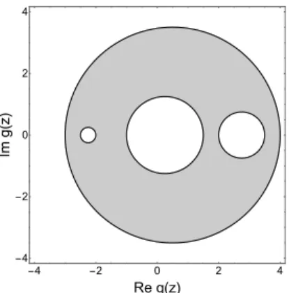
Qualitative analysis of the region of invertibility of Green’s function is performed in the case of eigenvalue densities supported on a finite number of intervals and further refined by considering invariant random matrix ensembles. We provide conditions for the appearance of singularities during a continuous deformation of matrix models in question.

(4)

Kurzzussamenfassung

Wir betrachten allgemeine Ensembles von N×N Zufallsmatrizen im Limes von großer Matrixgröße (N→ ∞). Unser Ziel ist es eine neue Vorge- hensweise zu etablieren, um lokalen Eigenwertstatistiken zu analysieren und dadurch die Grenzen der bekannten Universalitätsklassen, ohne strenge An- nahmen über die Wahrscheinlichkeitsmaße von Matrix- Ensemble, zu erweit- ern. Das Problem der Berechnung von n-Punktkorrelationsfunktion wird mittels der supersymmetrischen Verallgemeinerung der Laplace-Transfor- mation gelöst. Der Limes von großem N der Transformation von Parti- tionsfunktionen wird in vielen Fällen durch die aus der freien Wahrschein- lichkeitstheorie bekannte R-Transformation bestimmt.

Wir beweisen die Existenz und Eindeutigkeit von supersymmetrischen Laplace-Transformation und ihre Inverse am Beispiel von interessanten Fäll- en, in denen ein Verhältnis von Determinantenprodukten erwägt wird. Uns- er Ausgangspunkt ist die in bestimmter Weise regularisierte Fourier Trans- formation im Raum Hermitescher Matrizen. Eine detaillierte Herleitung wird am Beispiel einer unitären Symmetrie gegeben, während Formeln für reelle symmetrische und quaternione selbstduale Matrizen jeweils aus der analytischen Struktur von Harish-Chandra-Itzyskon- Zuber Integral über orthogonal und symplektische Gruppen folgen.

Die Reichweite von Anwendbarkeit unserer Methode wird durch eine ein- fache Formel gezeigt, ohne auf irgendwelche Annahmen über die Form der Wahrscheinlichkeitsdichte zu beruhen. Daraus wurde Formalismus entwick- elt, der sowohl Standardfälle von Wigner als auch invariante Zufallsmatrix- Ensembles umfasst. Wir entwickelnN → ∞Anwendbarkeitsbedingungen in einer Weise, die uns ermöglicht die Größenordnung von Fehlerterm für großenN zu kontrollieren.

iv

(5)

1 Introduction

1.1 Outline

This thesis is organized in the following way. In chapter 1 we provide the motivation for our work and a short historical background of the research done in the area of random matrix theory. We explain the basic ideas of two main theories we use and combine throughout the thesis. The free probability theory is introduced in section 1.2.2 and the second one, the supersymmetry, is briefly described in section 1.3. The combination of those two formalisms is the main topic of this thesis. We close the chapter by reviewing previous results in the area of correlations between random matrix eigenvalues in section 1.4.

Chapter 2 covers the construction of the main object of interest in this thesis, the Laplace transform in space of supermatrices. We start by introducing relevant objects and motivating the need for said transform in the random matrix theory. Next, in section 2.1, we show in a heuristic way a connection between the Laplace transform of partition function for the correlation functions of random matrix eigenvalues with the supersymmetric extension of the R-transform known from the free probability theory. We proceed with the explanation of how our formalism applies in simplest cases of 1-point function in section 2.2 and continue by showing how one can extend it to many-point correlations in sections 2.3 and 2.4. We use techniques of complex analysis, i.e. contour integrations and analytic continuations to prove existence and invertibility of Laplace transform of partition functions describing correlations between random matrix eigenvalues. The derivation is based on well established Fourier transform in space of matrices. In the beginning, we restrict ourselves to the case of unitary symmetry, or in other words to the transforms over space of Hermitian matrices. Last section, 2.5, is devoted to the extension of our formalism to other symmetry classes, i.e. orthogonal and symplectic, related to real symmetric and quaternion self-dual matrices respectively.

The goal of chapter 3 is to determine the region of applicability of our approach. We give a simple requirement that is necessary for all approxi- mations in our derivation to be exact in the large matrix size limit (often referred to asN → ∞limit). In chapter 4 special attention is placed on the regions of invertibility of Green’s function and as a consequence of the inverse function theorem, analyticity of the R-transform. We start with

(8)

1. Introduction

general considerations, but to obtain more quantitative results, we restrict ourselves first to the case of the eigenvalue distribution supported on a few intervals in section 4.1 and later to invariant random matrix ensembles in section 4.2.

Chapter 5 summarizes the thesis and describes consequences of our results. We give an outlook on possible extensions and further developments that may be accessible thanks to our Laplace transform formula.

1.2 Random matrices 1.2.1 Overview

Matrices play many roles in mathematics, physics, data analysis, telecom- munication, and other numerous topics.The first work where considered matrix was taken to have random elements, was done by Wishart [1], where the correlation coefficients of multivariate data samples were computed, though his work did not get deserved recognition at the time. The real pioneering work in the field is attributed to Wigner [2]. In nuclear physics context Wigner devised a model for Hamiltonians of heavy nuclei - too complicated to write down and compute explicitly, therefore assumed to be represented by large matrices with independent random Gaussian entries with appropriate symmetries. Model turned out to describe spacings between energy levels (eigenvalues) quite well, but what is more important, is the fact that many different nuclei displayed similar level spacings, exhibiting a property called ’level repulsion’. The statistics of eigenvalues of random Hamiltoni- ans were far from Poisson that would be expected from uncorrelated variables, showing that even though elements of the matrix are independent, the eigenvalues become highly correlated. The universality of the result suggests additionally, that the local statistics are independent of details of the system but depend only on general properties like symmetries or band structure. Eigenvalues statistics are so far the most studied property of random matrices, but there has been some interest in other quantities like e.g.

eigenvectors. For a more detailed historical introduction see [3].

One of the most common ways of constructing random matrix models is to consider matrices with, up to symmetry, independent entries. A special class of those, called Wigner matrices, is constructed by requiring all elements above diagonal to have zero mean and identical second moment and requiring elements below the diagonal to reflect matrix symmetry (e.g.

invariance under transposition or hermitian conjugation). A prime example from this class is a random matrix with all elements above diagonal being independent identically distributed standardized complex Gaussian random numbers, while diagonal ones are real.

The second convenient way of description is by a probability measure on space of matrices that is invariant with respect to transformation by some symmetry group. Standard example being random measures on space of Hermitian matrices invariant w.r.t. unitary transformation. Each such measure can be written in the following form:

µ(H)∝e^−TrV^(H) , (1.1)

2

(9)

1.2. Random matrices

whereV (x) is a real-valued function (ensuring positivity of the probability measure), called a potential - often considered to be a polynomial of small degree.

Three classical random matrix models are the Gaussian Orthogonal En- semble, Gaussian Unitary Ensemble, and Gaussian Symplectic Ensemble.

They all belong to both classes of Wigner and invariant random matrices and differ only by symmetry group. One can construct them by taking elements to be independent Gaussian random variables with mean zero and appropriate variance - ensuring invariance property. In the first case the matrix is real and symmetric, in second situation it is complex and Hermitian and in the third case, one considers a self-dual quaternion matrix.

It has been shown that there is a total of 10 symmetry classes [4]. In this thesis, we will restrict ourselves to 3 mentioned before, called classical symmetry classes. In a typical way, we will start by considering the com- putationally simplest unitary symmetry and afterward show how one can extend the results to the orthogonal and symplectic symmetries.

1.2.2 Free probability

Many techniques were used in the study of random matrix models, in- cluding enumerative combinatorics, Fredholm determinants, diffusion pro- cesses or integrable systems just to name a few (see [5, 6] for reviews).

In this section we will focus on one of them, the theory of free probability, invented by Voiculescu [7] in the context of free group factors isomorphism problem in the theory of operator algebras. Free probability describes be- havior and properties of so-called ’free’ non-commutative random variables with respect to addition and multiplication of said variables. The ’freeness’

property is defined in the following way: two random variablesAandBare free with respect to a unital linear functionalφif for alln1, m1, n2, . . .≥1 we have:

φ((Aⁿ¹−φ(Aⁿ¹)1) (B^m¹−φ(B^m¹)1) (Aⁿ²−φ(Aⁿ²)1). . .) = 0, (1.2a) φ((Bⁿ¹−φ(Bⁿ¹)1) (A^m¹−φ(A^m¹)1) (Bⁿ²−φ(Bⁿ²)1). . .) = 0.

(1.2b) It basically allows one to compute mixed moments from moments of indi- vidual random variables, e.g. freeness ensures that:

φ(AⁿB^m) =φ(Aⁿ)φ(B^m). (1.3) Soon after it was realized [8] that large independent random matrices with uncorrelated eigenvectors are mutually free with respect to the limN→∞ 1

NE{Tr (•)}functional.

Let us introduce main objects needed when dealing with random matrices in the free probability setting. Firstly, for aN×NHermitian matrixHone has the empirical eigenvalue distribution:

ρH(λ) = 1 N

N

X

i=1

δ(λ−λi) , (1.4)

(10)

1. Introduction

where{λi}are eigenvalues ofH. Now instead of considering a single deter- ministic matrix, we can move on to an ensemble of random matrices defined by some probability measureµN(H) and define the average eigenvalue density by:

ρN(λ) =E (1

N

X

i=1

δ(λ−λi) )

= Z 1

N

X

i=1

δ(λ−λi)dµN(H) . (1.5)

We are also going to assume that the limit limN→∞ρN(λ) converges to a probability measureρ(λ). The form of eq. (1.5) is not very convenient for applications, because a measure on the space of matrices expressed in terms of its eigenvalues will either be very complicated to integrate or, e.g.

in the case of uncorrelated eigenvalues, not interesting. Therefore one often rewrites it using following representation of real Dirac delta:

δ(λ) =−1 π lim

→0⁺Im 1

λ+i . (1.6)

Next, we define a Green’s function as the Stieltjes transform of eigenvalue distribution and we can recover said distribution by taking the imaginary part of Green’s function and approaching the eigenvalue support on the real line from the complex plane:

g(z) = Z

R

ρ(λ)

z−λdλ= lim

N→∞N⁻¹E n

Tr (z1−H)⁻¹ o

, (1.7)

ρ(λ) =−1 π lim

→0⁺Img(λ+i) . (1.8)

The Green’s function is analytic in the complex plane away from the eigenvalue distribution, therefore it can be expanded into a series around z=∞and presented as a moment generating function:

g(z) = lim

N→∞N⁻¹E

Tr z⁻¹+z⁻¹Hz⁻¹+. . . =

∞

X

k=0

z^−k−1mk, (1.9)

mk= lim

N→∞

1 NE

n TrH^k

o

. (1.10)

This is an analog of the moment generating function known from standard commutative probability theory. We can see that knowledge of all moments allows one to determine the average eigenvalue distribution, therefore all result of the free probability apply to average eigenvalue spectra of large random matrices.

Recall that in regular commutative probability theory one can obtain a distribution of a random variable constructed as a sum of independent random variables via sum of cumulant generating functions of the summands, therefore in the setting of free probability we want to have an analogue of cumulant generating function for average eigenvalue distribution that would be additive w.r.t. addition of random matrices. For non-commutative variables this object is defined via its relation to Green’s function and called the

4

(11)

1.3. Supersymmetry

R-transform. Not going into details that were derived in [7], the R-transform and free cumulantsκnare defined as follows:

g(z) = 1

z−R(g(z)) , (1.11)

R(w) =X

n=1

κnwⁿ⁻¹, (1.12)

with the inverse relation

R(w) =g⁻¹(w)−w⁻¹ . (1.13) Having defined all necessary objects, the addition law for free random ma- tricesAandBreads:

RA+B(z) =RA(z) +RB(z) . (1.14) Another question that arises is: can free probability theory provide information about eigenvalue spectra of products of random matrices? Even though the product of two Hermitian matrices is not Hermitian and in principle the formalism breaks down because the eigenvalue density of a product is not supported on the real axis anymore, in some cases, one can also devise the multiplication law in terms of R-transform [9]. We can consider a product of two free Hermitian matricesA, BassumingA- positive semi-definite and instead consider an equivalent problem of computing eigenvalues of the productA^1/2BA^1/2. In those cases one has a closed set of equations:

RAB(z) =RA(w)RB(v) , (1.15a)

v=zRA(w) , (1.15b)

w=zRB(v) . (1.15c)

The R-transform will be of great importance for us for reasons explained later, but it’s worth mentioning now that if one is interested only in the average eigenvalue distributions one doesn’t need to calculate R-transforms. The recently developed theory of subordination [10, 11] allows one to efficiently linearise and compute Green’s function for polynomials and rational expres- sions in random matrices. This method doesn’t reference the R-transform, which in principle might not be well defined in parts of the complex plane, therefore has to be handled with care and might not be a convenient object to manipulate numerically. I.e. R-transform is properly defined on circular sectors around the origin of the complex plane. We focus on the analysis of the analytic structure of the R-transform in chapter 4.

1.3 Supersymmetry

1.3.1 Grassmann variables

The first step in the introduction of the supersymmetry method is to recall basic information about the Grassmann variables, denoted throughout

(12)

1. Introduction

this section by Greek lettersχiwithi= 1, . . . , n. They are elements of the Grassmann algebra and obey anticommutation relations:

{χ_i, χj}=χiχj+χjχi= 0 for any 1≤i, j≤n . (1.16) Anticommutation rules imply in particular, by takingi=j, that

χ²_i= 0. (1.17)

The usage of Grassmann variables in physics was significantly expanded by the introduction of the Berezin integral [12] over anticommuting variables.

This integral is formally defined by two simple rules Z

dχi= 0, (1.18)

Z

χidχi= 1, (1.19)

sufficient to integrate arbitrary function due to eq. (1.17). Any function of a single Grassmann variable must be linear in this variable and integrals of sums are taken to be equal to sums of integrals.

For the physical application, the most important Berezin integrals are the Gaussian integrals. As a further consequence of eq. (1.17), any series expansion of an analytic function of a Grassmann variable ends with the second term. Knowing that, it is easy to check by direct computation the following identity

Z exp

−χ¯^TAχYⁿ

i=1

dχ¯idχi= DetA , (1.20)

where{χ_i}and{χ¯i}are two sets of independent Grassmann variables and χand ¯χrepresent vectors ofχiand ¯χirespectively. A standard counterpart of this formula is the Gaussian integral over complex variablesψi:

Z exp

−ψ^†Aψ Yⁿ

i=1

dψ¯idψi=πⁿDet⁻¹A . (1.21) Because of this analogy, some texts refer to ¯χi as a complex conjugate of χi but in principle there is no need to try to add this structure because ψi and ¯ψiare independent variables in the same sense asχi and ¯χi. The difference amounts to a change of basis, with respect to which determinants are invariant.

1.3.2 Supervectors and supermatrices

One can extend standard linear algebra by introducing an additional anticommutative structure. An (n|m) supervector Θ is defined as a vector with block structure

Θ = χ

b

, (1.22)

6

(13)

1.4. Previous results

whereχis anncomponent vector of Grassmann variablesχi and bis an mcomponent vector of complex numbersbj. A product of a complex and Grassmann numbers results in an anticommuting variable, while a product of two Grassmann numbers is, in turn, a commuting object. Therefore if we want to define linear transformations preserving the block structure of Θ, we need to represent them by matrices with a matching block structure:

A=

A00 σ ρ A11

, (1.23)

whereA00andA11are matrices of sizen×nandm×mrespectively, consisting of commuting variables, whileσandρaren×mandm×nmatrices with anticommuting elements. Such extensions of vectors and matrices are called supervectors and supermatrices.

Lastly, one needs the extension of basic operations on supermatrices.

Using notation of eq. (1.23), the generalization of the trace of a matrix, preserving invariance w.r.t. cyclic permutations, called a supertrace is defined as

STrA= TrA00−TrA11, (1.24)

while equation defining a superdeterminant (also called Berezinian) is in turn determined through

ln SDetA= STr lnA . (1.25)

IfA00 and A11 are invertible, one has another way of expressing the superdeterminant:

SDetA= Det (A00) Det⁻¹

A11−ρA⁻¹₀₀σ

(1.26a)

= Det

A00−σA⁻¹₁₁ρ

Det⁻¹(A11) . (1.26b) Combining both commuting and anticommuting variables into one formalism significantly simplifies the notation, e.g. the Gaussian integral over complex and Grassmann variables gives

Z exp

−Θ¯^TAΘYⁿ

i

d¯χidχi m

Y

j=1

d¯bjdbj=π^mSDetA . (1.27)

1.4 Previous results

As mentioned before, it is believed that many of the local eigenvalue statistics, like e.g. distribution of spacings between neighboring levels, are universal, that is independent of the details of random matrix model. There are many quantities of interest one can inspect on the local level, the simplest being aforementioned level spacing or distribution of sayk’th largest eigenvalue. The object that possesses the most information about eigenvalue statistics is their joint probability distribution function (jpdf) denoted byρN(λ1, . . . , λN) (for a Hermitian matrix of sizeN×N) where we take λ1 ≤. . . λN. For simplicity of notation, we use ¯ρN for jpdf symmetrized

(14)

1. Introduction

w.r.t. eigenvalue permutations. From the jpdf one can recover any eigenvalue statistics, the simplest being average eigenvalue density:

ρ(λ) = Z

Rⁿ⁻¹

¯

ρ(λ, λ2, . . . , λN)dλ2. . . dλN, (1.28) or a singlek’th eigenvalue distribution

ρ(λk) = Z

Rⁿ⁻¹

ρ(λ1, . . . , λN)dλ1. . . dλk−1dλk+1. . . dλN. (1.29) In a similar manner, one defines k-point correlation functions

ρ^k(λ1, . . . , λk) = Z

R^n−k

¯

ρN(λ1, . . . , λN)dλk+1. . . dλN . (1.30) The universality of statistics tells us, that we need to be able to compute them only in one simple case to know the result in any more complicated situation falling into the same universality class. Obvious choice for the specific model for computation is the most symmetric one - GUE, defined by the probability measure

dµ(H)∝e^−TrH²^/2dH . (1.31) In this case one has explicit formulas for jpdf and all other correlation functions, having an exceptionally simple form

ρ^k(λ1, . . . , λk) = det (K(λi, λj))_1≤i,j≤k , (1.32) K λ√

N+ x

√

N ρsc(λ), λ√

N+ y

√ N ρsc(λ)

!

(1.33)

−−−−→

N→∞ KSine(x, y) =sin (π(x−y))

π(x−y) , (1.34) whereρsc(λ) =_2π¹√

4−λ²1|λ|≤2is the average eigenvalue density for properly rescaled GUE, called the Wigner semicircle distribution, and|λ|<2.

The universality of eigenvalue statistics is known as ”Sine kernel universality”, thanks to the interpretation of eigenvalues of random matrices as particles in a determinantal point process with kernelKSine(x, y). Many works were devoted to proving and expanding regions of validity of the universality conjecture, in both realms of Wigner and invariant random matrices. We will shortly describe previous results and refer the reader to some of the extensive literature on the subject.

1.4.1 Wigner matrices

First of the methods to analyze the local statistics of Wigner matrices are the heat flow techniques. One starts with a Wigner matrix, say M_N⁰, and considers a stochastic diffusion process defined by the equation

dM_N^t =dβt−1

2M_N^tdt , (1.35)

8

(15)

1.4. Previous results

with a starting point atM_N^t |t=0=M_N⁰. βt is a Hermitian matrix process with entries being independent Brownian motions, real on the diagonal, complex off the diagonal. This process describes a continuous flow from M_N⁰ towards GUE ast→ ∞. Roughly speaking, one can use the dynamics of the flow of eigenvalues, established by Dyson [13], to extend the Sine kernel universality [14, 15].

Another way of dealing with Wigner matrices is the so-called ’Four Mo- ment Theorem’. The theorem asserts that statistics of the eigenvalues on the local scale ofN^−1/2depend only on the first four moments of the matrix entries [16]. Details of that approach are beyond the scope of this thesis, but by using the Four Moment Theorem the universality has been proven for a broad class of Wigner hermitian matrices [17] and further extended to properties of eigenvectors [18] and eigenvalues of non-hermitian random matrices [19]. For a detailed review on the topic of universality in the class of Wigner random matrices see [20].

1.4.2 Invariant ensembles

Some work has been done in the case of invariant ensembles, starting with [21], where Sine kernel universality was shown for invariant unitary random matrices with potential function having sufficiently fast growing tails. The method of proof was relying strongly on the orthogonal polynomial technique. This method proved to be very effective in the case of analytic potentials with some additional requirements [22, 23, 24] and a lot of progress was made (see [25] for a review), though often restricted to the unitary symmetry class only.

More recent results proving universality hypothesis for a broader class of random matrix ensembles came from flow equation approach [26, 27] applied to so-calledβ-ensembles, an interpolation between the 3 classical symmetry classes. Similar to the case of Wigner matrices, one can investigate a flow in space of invariant matrices ending with the Gaussian ensemble, in this way matching the statistics of complicated models with the Gaussian ones.

Lastly, first results combining formalisms of supersymmetry and free probability came in [28], while the first attempts to relate the Laplace transform of partition function with free probabilistic R-transform arose in [29].

The relation was proven for different regimes for a low-rank argument of the transform in several papers. [30] showed the result in the case of eigenvalue distribution restricted to an interval, while [31] proved the matching in the case of analytic uniformly convex potentials. We expand and generalize those results.

(16)

(17)

2 Laplace transform

In the standard setting, the Laplace transform of a functionf(p) is defined forq≥0 by:

f˜(q) = Z ∞

0

f(p)e^−pqdp . (2.1)

Formally, to invert the transform one performs an integral in the complex plane, parallel to the imaginary axis:

f(p) = 1 2πi

Zγ+i∞

γ−i∞

f˜(q)e^pqdq , (2.2)

whereγ∈Ris greater than the real part of singularities of ˜f(q). In practice, one can close the contour of integration to the left of the complex plane and have it encircling all singularities of ˜f(q).

Our goal is the description of correlation functions for eigenvalues of random matrix models. As explained in section 1.2.2, the average eigenvalue density (one-point correlation function) may be obtained by considering the Green’s function, i.e.:

g(z) = lim

N→∞N⁻¹E n

Tr (z1−H)⁻¹ o

, (2.3)

whereH is aN×N random matrix. Trace may be expressed as a ratio of determinants, giving us an alternate expression for the resolvent:

g(z) = lim

N→∞N⁻¹E d

dz⁰

Det (z⁰1−H) Det (z1−H) z⁰=z

. (2.4)

In a similar manner, the many-point correlation functions are governed by the expected value of a ratio of products of determinants. We define a general (n|m) partition function by:

Z_n|m({p0},{p1}) =E ( Qm

j=1Det (p1,j1−H) Qn

k=1Det p_0,k1−H )

. (2.5)

This object extends to a radial function of a supermatrixP of rank (n|m):

Z(P) =E

SDet⁻¹ P⊗1N−1_n|m⊗H . (2.6)

(18)

2. Laplace transform

The goal of this chapter is to establish and prove the existence of the Laplace transform and its inverse in the context of the supersymmetric generalization of the aforementioned partition function (2.6), first in the case of one-point function as a proof of concept, and later for arbitrary integer values ofnandm.

It remains to motivate the need for Laplace transform in the random matrix theory. What is the advantage of taking Laplace transform of our partition function? Then= 1,m = 0 example is enough to see the idea.

We use the notation G(p) = lim

N→∞GN(p) = lim

N→∞N⁻¹E{Tr ln (p1−H)} , (2.7) for so-called integrated Green’s function, related to the standard Green’s function by:

g(p) = ∂

∂pG(p) . (2.8)

One can reduce the expected value of a determinant into a simpler form using the following approximation:

Z(p) =E

Det⁻¹(p1−H) (2.9a)

=En

e−Tr ln(p1−H)o

(2.9b)

≈e−E{Tr ln(p1−H)} (2.9c)

=e^{−N G}^N^(p). (2.9d)

Unfortunately, whenpis near the spectrum ofH it is a bad approximation.

The way to avoid it would be to keep p away from support of eigenvalue distribution ofHby e.g. performing the following transformation:

Z˜(q) = I

E

Det⁻¹(p1−H) e^pqdp , (2.10)

with the contour of integration encircling the support of the spectrum. Af- ter performing this approximation, all calculations are reduced to one-point functions, therefore it cannot be true for any probability density. One can construct many random matrix models with same average eigenvalue density and very different correlation functions. E.g. one can choose each eigenvalue as an independent random variable distributed identically to the GUE average eigenvalue spectrum, in the first case one has Poisson statistics, vastly different from ones observed in the latter case. Validity of this approximation is discussed in detail in chapter 3. After making the approximation, one way of evaluating this integral (or in more complicated cases its supersymmetric extension) inN→ ∞limit is to perform a saddle-point analysis.

This form resembles the inverse Laplace transform, making it a topic worth further investigation.

12

(19)

2.1. R-transform as a result of the saddle-point approximation

2.1 R-transform as a result of the saddle-point approximation

In this section, we heuristically explain the connection between supersymmetry, free probability and local statistics of eigenvalues. We leave out many details, like e.g. normalization constants or integration domains, that are derived and explained in later parts of the thesis. For simplicity, the notation used in this section is schematic and not mathematically precise.

As discussed in the previous section, we want to calculate the Laplace transform of a supersymmetric partition function (2.6) that is schematically expressed as

Z˜(Q) = Z

dPexp (STrP Q)Z(P) (2.11a)

= Z

dPexp (STrP Q)E

SDet⁻¹(P⊗1−1⊗H) , (2.11b) whereQandPare supermatrices of appropriate sizes and symmetries. Now we assume that inN → ∞ limit we can move the expected value under the exponential. Denoting a supersymmetric lift of the integrated Green’s function byG(P) we arrive at

= Z

dPexp (STrP Q) exp (−STr logE{P⊗1−1⊗H}) (2.11c)

= Z

dPexp (STrP Q−NSTrG(P)) . (2.11d)

Now taking ˜Z(N Q) for largeN, we can perform a saddle-point approximation of the integral. We make a variation ofP in a direction of someδP and calculate a directional derivative of the exponent w.r.t. a parametert.

The matricesP0for which the derivative vanishes form a critical subspace STr (δP Q)− lim

t→0STrG(P+tδP)−G(P) t

P=P₀

= 0. (2.12) Writing the lift of Green’s function as

g(P) = lim

N→∞N⁻¹En

P⊗1−1n|m⊗H−1o , and requiring condition (2.12) to be true for anyδP, we have:

Q−g(P0) = 0, (2.13)

resulting in

Γ (Q) : = logN⁻¹Z˜(N Q)∝STr (P0Q−G(P0))

= STr g⁻¹(Q)Q−G g⁻¹(Q)

. (2.14)

The last step is to again take a derivative (this time simply denoted by prime symbol ”⁰”) and remove the singularity atQ= 0, resulting in

(Γ (Q)−STr logQ)⁰= STr g⁻¹(Q)−Q⁻¹

, (2.15)

which has exactly the form of eq. (1.13), defining the R-transform, or in this case a supersymmetric extension thereof.

(20)

2.2 One-point function

We use the one-point function as an example allowing us to present the reasoning behind the more complicated analysis of the Laplace transform for many-point correlation functions. The main idea is to start with the well- established Fourier transform and to use techniques of complex analysis, i.e.

contour integration and analytic continuations in order to establish relations between the transforms. The standard Fourier transform and its inverse are given by:

fˆ(q) = Z ∞

−∞

f(p)e^−ipqdp , (2.16)

f(p) = 1 2π

Z ∞

−∞

fˆ(q)e^ipqdq . (2.17)

2.2.1 Fermion-fermion sector

In this section we will consider the relation between Fourier and Laplace transforms of the function:

f(p) = Det (p1−H). (2.18)

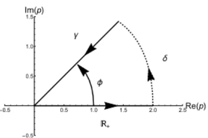
which is a polynomial in variablep, and therefore doesn’t have any singularities. The Laplace transform, defined for Re (q) > 0, extends to a holomorphic function onC\ {0}by following an analytic continuation procedure. We start by drawing a contour of integration consisting of real positive semi-axis, another ray starting at the origin and lying in the right side of the complex plane, denoted byγ, and an arc connecting those two in the infinity as presented in fig. 2.1. We performH

f(p)e^−pqdpalong this contour in the counter-clockwise direction and using Cauchy integral theorem we know that such integral is equal to zero. Therefore, as the integral on the arc in infinity vanishes, we know that

Z ∞ 0

f(p)e^−pqdp=− Z

γ

f(p)e^−pqdp= Z

−γ

f(p)e^−pqdp , (2.19) where the two integrals are properly defined. If we denote byαthe angle between real positive semi-axis andγ, the integral overγis well defined in the region described by inequality

Re (q) cosα−Im (q) sinα >0. (2.20) In fact, we can define the analytical continuation of Laplace transform for anyq∈C/{0}by repeating this procedure. In particular, we have

f˜(q) = Z −∞

0

f(p)e^−pqdp , (2.21)

for Re (q)<0.

Let us turn our attention to the Fourier transform off(p). It’s not well defined unless we perform some regularization procedure. We will regularize

14

(21)

2.2. One-point function

ℝ+

ϕ

δ γ

-0.5 0.5 1.0 1.5 2.0 2.5Re(p)

-0.5 0.5 1.0 1.5

Im(p)

Figure 2.1: Sketch of the contour of integration used for analytical continuation of the Laplace transform in the fermion-fermion sector. Integral over the real positive semi-axis coincides with integral over (−γ) as there are no singularities inside of the contour and integral overδvanishes.

the transform by using an exponential cutoff and relate it to the Laplace transform:

fˆ(q) = lim

→0⁺

Z∞

−∞

f(p)e^−ipqe^−|p|dp (2.22a)

= lim

→0⁺

Z ∞ 0

f(p)e^−ipqe^−pdp− Z −∞

0

f(p)e^−ipqe^pdp

(2.22b)

= lim

→0⁺

f˜(ip+)−f˜(ip−)

. (2.22c)

Having this relation, we can use the inverse Fourier transform to construct the inverse of the Laplace transform in turn showing it’s existence and form. The inverse relation goes as follows,

f(p) = 1 2π

Z ∞

−∞

fˆ(q)e^ipqdq (2.23a)

= lim

→0⁺

1 2π

Z∞

−∞

f˜(iq+)−f˜(iq−)

e^ipqdq (2.23b)

= lim

→0⁺

1 2π

Z ∞−i

−∞−i

f˜(iq)e^ipqdq− Z ∞+i

−∞+i

f˜(iq)e^ipqdq

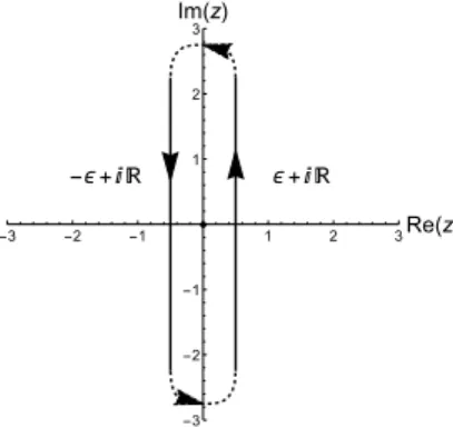
. (2.23c) After a change of the integration variable toz :=iq, the two integrals can be collapsed to a contour integral running counter-clockwise around the imaginary axis (see fig. 2.2). Any contour deformation is allowed, as long as it doesn’t pass through the possible singularity at 0. Therefore we end with the following inverse Laplace transform:

f(p) = 1 2πi

I

f˜(z)e^pzdz , (2.24) where integration contour encircles the origin of the complex plane.

(22)

ϵ+ⅈ ℝ -ϵ+ⅈ ℝ

-3 -2 -1 1 2 3Re(z)

-3 -2 -1 1 2 3

Im(z)

Figure 2.2: Sketch of the contour of integration used for calculation of the inverse Laplace transform in the fermion-fermion sector. We join two integrals over lines parallel to the imaginary axis, one slightly to the right, and one slightly to the left, in±i∞, in turn replacing them by one contour integral around the imaginary axis.

2.2.2 Boson-boson sector

Regularization of the denominator in the Green’s function can be done in one of two ways, advanced or retarded, denoted in this section by

f(p) = Det⁻¹(p1±i−H) . (2.25) For the simplicity we will consider only the advanced case, the other one is analogical. Let us again start with the Fourier transform, adjust contours and arrive at Laplace transform and its inverse in the boson-boson sector.

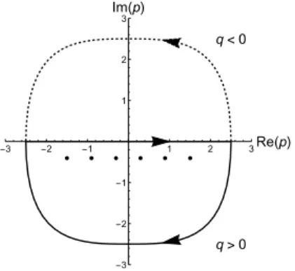
Starting with the integral over the real axis, we close the contour of integration in either upper or lower complex plane, depending on the sign of the transform argument (see fig. 2.3). Therefore we have:

fˆ(q) = Z ∞

−∞

f(p)e^−ipqdp= I

κ

f(p)e^−ipqdp , (2.26)

whereκgoes along the real axis to the right and closes in the upper complex plane forq <0 or lower forq >0.f(p) is holomorphic in the upper complex plane, so again using Cauchy theorem we obtain that ˆf(q) = 0 forq <0.

In case ofq >0, we may deform the contour into any shape encircling all singularities off(p), that is positions of the eigenvalues shifted byiinto the lower complex plane. After making thep→ipvariable change, we end up with the following reduced formulas for the Fourier transform and its

16

Free probability approach to microscopic statistics of random matrix eigenvalues