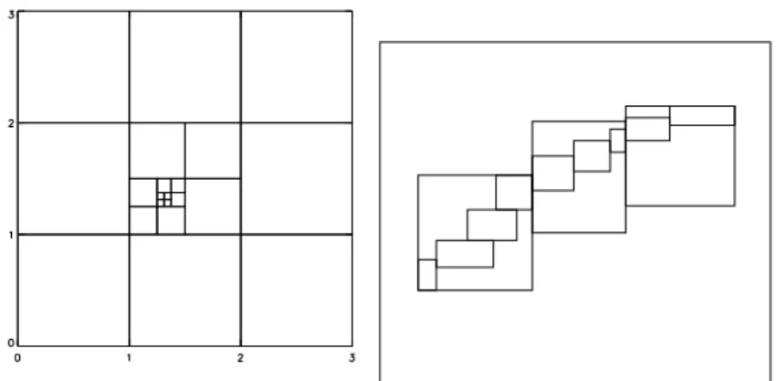
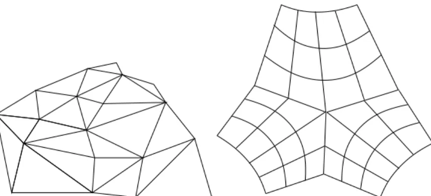
Chapter 10 Coordinate systems and gridding techniques
11
0
0
Volltext
(2)
(3)
(4)
(5)
(6)
(7)
(8)
(9)
(10)
(11)
Abbildung
ÄHNLICHE DOKUMENTE
(Ahiran §ä'a-ra§ul al-muntazar, „Endlich ist der erwartete Mann gekommen", in: Ahmad H. az-Zaiyät, Wahy ar-Risäla, Bd. 1954 schreibt "Abd an-Näsir in seiner „Philosophie
Fauna that settle on such hard substrates are very exciting to specialists dealing with these kinds of animals; however, those that are investigating animals of the Larsen B
The purpose of the current paper is to reconsider the case of conservation laws in the Lagrangian and Hamiltonian systems used in both classical Wal- rasian equilibrium theory 2 and
The basic problern here address'ed can be stated as folIows: could the north polar ice cap of Mars remain in an almost steady state by ice flow from a central area with net
Функциите на изпълнителната власт могат да се осъществяват и в съответствие с принципа на деконцентрацията, разбирана като разпределение
Hagedorn and I now have preliminary evidence that extirpation of the neurosecretory system will prevent the ovary from secreting ecydsone after a blood meal, and as a consequence
The company has continued to flourish and has performed in over 50 countries around the world, at venues such as the Purcell Room of the Royal Festival Hall and the Victoria and
Figure 1: Ice flow (white arrows) and divergence (top row, in 10 −7 s −1 negative values imply con- vergent flow) and bulk viscosities (bottom row, in N s m −1 , logarithmic scale)
