Tree Kernel Usage in Naive Bayes Classifiers

Tree Kernel Usage in Na¨ıve Bayes Classifiers

Felix Jungermann

Artificial Intelligence Group – Technical University of Dortmund felix.jungermann@cs.tu-dortmund.de

Abstract

We present a novel approach in machine learning by combining na¨ıve Bayes classifiers with tree kernels. Tree kernel methods produce promising results in machine learning tasks containing tree- structured attribute values. These kernel methods are used to compare two tree-structured attribute values recursively. Up to now tree kernels are only used in kernel machines like Support Vector Machines or Perceptrons.

In this paper, we show that tree kernels can be utilized in a na¨ıve Bayes classifier enabling the classifier to handle tree-structured values. We evaluate our approach on three datasets contain- ing tree-structured values. We show that our approach using tree-structures delivers signifi- cantly better results in contrast to approaches us- ing non-structured (flat) features extracted from the tree. Additionally, we show that our approach is significantly faster than comparable kernel ma- chines in several settings which makes it more useful in resource-aware settings like mobile de- vices.

Na¨ıve Bayes Classifier; Tree Kernel; Lazy Learning;

Tree-structured Values

1 Introduction

Na¨ıve Bayes classifiers are well-known machine learn- ing techniques. Based on the Bayes theorem the na¨ıve Bayes classifiers deliver very good results for many ma- chine learning tasks in practical use.

Many machine learning techniques like Support Vector Ma- chines (SVMs) or Decision Trees, for instance, are suf- fering from a complex training phase. Na¨ıve Bayes clas- sifiers do not have this disadvantage because the train- ing phase just consists of storing the training data ef- ficiently. In this way a na¨ıve Bayes classifier memo- rizes the training data by calculating probabilities using the observed values of the training data. Machine learn- ing techniques which memorize the training data instead of creating an optimized decision model are called lazy learners. In contrast to lazy learners like k-NN, for in- stance, na¨ıve Bayes classifiers do not memorize the com- plete training data. Nevertheless, na¨ıve Bayes classifiers create a condensed set of the training data which is not optimized. Although, na¨ıve Bayes classifiers are not op- timized, they deliver good results. Their ability to de- liver good results while not needing exhaustive training

makes na¨ıve Bayes classifiers to be preferred in resource- aware settings like mobile devices [Fricke et al., 2010;

Morik et al., 2010].

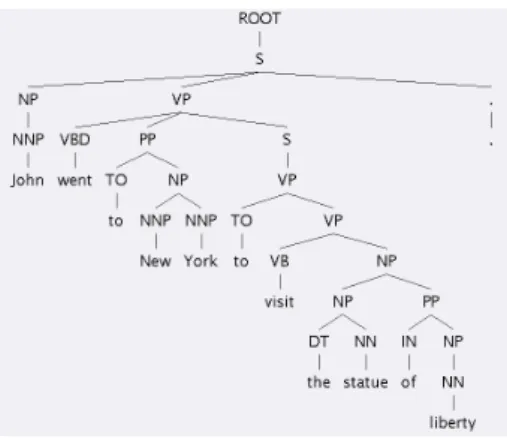
Unfortunately, memorizing specially shaped attribute values is not as trivial as it is for numerical or nominal at- tribute values. Tree-structured values for instance are fre- quently occurring in natural language processing or doc- ument classification tasks. Figure 1 shows a constituent parse tree of a sentence. This structured attribute might be helpful to detect and classify relations in this sentence. But it is not useful to store all trees seen in the training set. On the one hand the storage needs are too high, and on the other hand it is very unlikely that an exactly equal tree oc- curs in training and test phase.

Figure 1: A constituent parse tree

Tree kernels (see Section 3) allow a more flexible cal- culation of similarities for trees. Current machine learning approaches which respect tree-structured attribute types by using tree kernels are based on kernel machines. Suffering from relatively complex training, these techniques are not useful in resource-aware settings like mobile devices, for instance. Our contribution in this paper is threefold: we show how to embed tree kernels into na¨ıve Bayes classi- fiers. We present many options to handle the tree kernel values in a na¨ıve Bayes classifier, and we evaluate our tree kernel na¨ıve Bayes approach on three real-world datasets.

We will present already existing related work in this field of research in Section 2. Section 3 describes the handling of tree-structured values by using special kernels in kernel methods. In Section 4 we will show how a na¨ıve Bayes classifier is working. And in Section 5 we will show how to efficiently embed tree kernels in a na¨ıve Bayes classifier.

In Section 6 we will demonstrate the experiments we made on three datasets containing tree-structured attribute values.

Section 7 sums up our paper.

2 Related Work

To the best of our knowledge tree kernels never have been embedded in na¨ıve Bayes classifiers before. In the follow- ing we will show in which domains tree kernels have been used in SVMs to solve many diverse problems.

Tree kernels are very popular in relation extraction [Zhang et al., 2006; Zhou et al., 2007; Nguyen et al., 2009].

Pairs of named entities are representing relation candidates which have to be classified by machine learning techniques.

Tree kernels are used in this task to evaluate the parse tree structure spanning the context of both entities in the corre- sponding sentence. [Bloehdorn and Moschitti, 2007] have used tree kernels for text classification. They tested their approach on question classification and clinical free text analysis. Both are tasks which have formerly mostly been processed by using the bag of word (BOW) representation.

BOW is a representation which destroys the structure of the text, and machine learning methods cannot benefit from the structure anymore.

In addition, tree kernels have been used addressing an- other interesting and currently popular topic: sentiment analysis [Jiang et al., 2010]. Like for relation extraction two entities were used for this approach. The first entity is an opinion and the second entity is a product. The parse tree spanning the context of both entities is used to clas- sify the corresponding pair. [Moschitti and Basili, 2006]

used tree kernels for question answering. [Bockermann et al., 2009] used tree kernels to classify SQL-requests. The SQL-requests were parsed to get an SQL-tree which can be used for classifying those requests.

But SVMs are not the only machine learning technique tree kernels were used in. [Aiolli et al., 2007] showed that tree kernels can be efficiently embedded into perceptrons which can be used for online-learning.

3 Tree Kernels

Tree kernels are creating a mapping of examples into a tree kernel space providing a kernel function to compute the in- ner product of two tree elements. Tree kernels offer some sort of distance measure for trees delivering a real valued output given two trees. The usage of tree kernel meth- ods delivers best results in classification tasks offering tree- structured values like relational learning [Zhou et al., 2007;

Zhang et al., 2006].

The work of [Zhou et al., 2007; Zhang et al., 2006] is based on the convolution kernel presented by [Haussler, 1999] for discrete structures. To make the structural in- formation of a parse tree applicable by a machine learning technique a kernel for the comparison of two parse trees is used. This kernel compares two parse trees and delivers a real-valued number which can be used by machine learn- ing techniques. [Collins and Duffy, 2001] define a treek- ernel as written in eq. (1), where T

and T

are trees. N

and N

are the amounts of nodes of T

and T

. Each node n of a tree is the root of a (smaller) subtree of the origi- nal tree. I

(n) is an indicator-function that returns 1 if the root of subtree i is at node n. F is the amount of all subtrees which are apparent in the trees of the training data.

K(T

, T

) = X

n₁∈N1

X

n₂∈N2

|F |

X

i

I

(n

)I

(n

) (1)

= X

n1∈N1

X

n2∈N2

C(n

, n

) (2)

Creating the amount F is very complex. The question arises, if the computation of the eq. 1 could be done more efficiently. Instead of summing over the complete amount of subtrees F C(n

, n

) is used in eq. 2. C(n

, n

) repre- sents the number of common subtrees at node n

and n

. The number of common subtrees finally represents a syn- tactic similarity measure and can be calculated recursively starting at the leaf nodes in O(|N

||N

|). Summing over both trees ends up in a runtime of O((|N

||N

|)

).

During this recursive calculation three cases are being respected:

1. If the productions at n

and n

are different, C(n

, n

) = 0

2. If the productions at n

and n

are the same and if n

and n

are preterminals, C(n

, n

) = 1

3. Else if the productions at n

and n

are the same and if n

and n

are not preterminals, C(n

, n

) = Q

j

(σ + C(n

, n

)), where n

is the j-th children of n

(in a uniform manner for n

) and σ ∈ {1, 0}.

The σ-value is used to switch between the subset tree kernel (SST) [Collins and Duffy, 2001; ?] and the subtree kernel (ST) [Vishwanathan and Smola, 2002; ?]. By using σ = 1 the SST is calculated, whereas for σ = 0 the ST is calculated. Trees containing few nodes by definition only result in small kernel-outputs. In contrast, larger trees can achieve larger kernel-outputs. To avoid this bias, [Collins and Duffy, 2001] established a scaling factor 0 < λ ≤ 1 which is used in two of the three cases for the kernel calculation:

2. If the productions at n

and n

are the same and if n

and n

are preterminals, C(n

, n

) = λ

3. Else if the productions at n

and n

are the same and if n

and n

are not preterminals, C(n

, n

) = λ

Q

j

(σ + C(n

, n

)) .

4 Na¨ıve Bayes Classifier

The na¨ıve Bayes classifier (NBC) [Hastie et al., 2003] as- signs labels y ∈ Y to examples x ∈ X . Each exam- ple is a vector of m attributes written here as x

, where i ∈ {1, ..., m}. The probability of a label given an ex- ample according to the Bayes Theorem is shown in eq.

(4). Domingos and Pazzani [Domingos and Pazzani, 1996]

rewrite eq. (4) by assuming that the attributes are indepen- dent given the category (Bayes assumption). They define the Simple Bayes Classifier (SBC) shown in eq. (5). The classifier delivers the most probable class y ∈ Y for a given example x = x

, . . . , x

, formally described in eq. (5).

p(y|x

, ..., x

) =

1,...,xm)

(3) p(y|x

, ..., x

) =

1,...,x_m)

Q

j=1

p (x

|y)(4) arg max

y

p(y|x

, ..., x

) =

1,...,x_m)

Q

j=1

p (x

|y)(5) The term p (x

, ..., x

) can be neglected in eq. (5) be- cause it is a constant for every class y ∈ Y . The de- cision for the most probable class y for a given example x just depends on p(y) and p (x

|y) for i ∈ {1, . . . , m}.

One is using the expected values for the probabilities cal-

culated on the training data. The values can be calculated

after one run on the training data. The training runtime

is O(n), where n is the number of examples in the train-

ing set. The number of probabilities to be stored during

training are |Y | + P

j=1

|X

||Y |

for nominal attributes, where |Y | is the number of classes and |X

| is the num- ber of different values of the jth attribute. If the attributes are numerical, just a value for mean and standard deviation have to be stored resulting in O (m|Y |) probabilities.

Most implementations of na¨ıve Bayes classifiers deliver the class y which results in the greatest outcome for eq.

(5) for a given example x. It is not stringently required to use values between 0 and 1. This becomes important in Section 5.3. It has often been shown that SBC or NBC perform quite well for many data mining tasks [Domingos and Pazzani, 1996; Huang et al., 2003].

5 Tree Kernel Na¨ıve Bayes Classifier

In Section 4 it became clear that the important parameters for the na¨ıve Bayes classifier are p(y) and p (x

|y). p(y) is not affected by attribute-values and therefore is not affected by tree-structured attributes, too. p (x

|y) is the crucial pa- rameter which should be regarded in the following. We distinguish three types of attribute value types: nominal, numerical and tree-structured value types.

For nominal attribute value types x

, p (x

|y) is calcu- lated by simply counting the occurrences of the particular values of x

for each class y ∈ Y . For numerical attribute value types x

, the mean (µ

) and the standard-deviation (σ

) of the attribute are used to calculate the probability density function for every class y ∈ Y as seen in eq. (6). A Gaussian normal distribution is expected, here.

p (x

|y) = 1

√ 2πσ

e

_xi−µi

σi

2

(6) The calculation of the probability for tree-structured at- tribute values is not that trivial. A simple approach would be just to store each unique tree-structured value and count its occurrences like for nominal attributes. But this ap- proach is not promising as it is too coarse. It is not very probable that many examples are containing exactly the same tree-structured value. We are presenting a more flex- ible approach which uses tree kernels for the calculation of the conditional probabilities p (x

|y) for tree-structured attribute values:

If an attribute x

is tree-structured the tree kernel-value v

for class y is calculated by applying a tree kernel on x

and on every tree-structure x

been seen in the training-set S together with class y as shown in eq. (7).

v

= f

(x

) = X

x_j∈x⁰|(x⁰,y⁰)∈S,y⁰=y

K(x

, x

) (7)

This value could be used like every numerical value (see Section 5.2). To calculate this sum of kernel calculations all the tree-structures which have been seen in the train- ing set have to be taken into account. But storing every tree-structure ever seen in the training-phase on its own in a list for instance has two major drawbacks: The stor- age needs and the numbers of kernel calculations are very high. To lower the storage needs and the number of kernel- calculations we use the approach presented by [Aiolli et al., 2007] to store all tree-structured values in a compressed manner.

5.1 Efficient tree access

A minimal directed acyclic graph (DAG) containing a minimal number of vertices is used to store all the tree- structures, having seen in the training set for a particular

attribute and class, together. This leads to an amount of

|Y | DAGs, where |Y | is the number of classes. The DAG G = (V, E) contains a set of vertices V consisting of a label on the one hand and a frequency value on the other hand. And the DAG contains a set of directed edges E connecting some of the vertices.

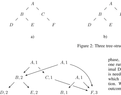
Figure 2 shows three trees which might occur during training for a specific class. A DAG containing all infor- mation being existent in these trees is shown in Figure 3.

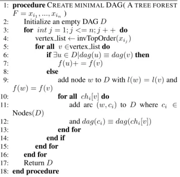
The algorithm to create a minimal DAG out of multiple trees is given in Algorithm ??. This algorithm converts ev- Algorithm 1 Creating a minimal DAG out of a forest of trees by [Aiolli et al., 2007]

1: procedure C

DAG( A

F = x

, ..., x

)

2: Initialize an empty DAG D 3: for int j = 1; j <= n; j + + do 4: vertex list ← invTopOrder(x

) 5: for all v ∈vertex list do

6: if ∃u ∈ D|dag(u) ≡ dag(v) then 7: f (u)+ = f (v)

8: else

9: add node w to D with l(w) = l(v) and f (w) = f (v)

10: for all ch

[v] do

11: add arc (w, c

) to D where c

∈ Nodes(D)

12: and dag(c

) ≡ dag(ch

[v])

13: end for

14: end if

15: end for 16: end for 17: Return D 18: end procedure

ery tree into its inverse topological ordered list of vertices.

The first elements of the list are vertices with zero outde- gree. After that vertices containing at most children with zero outdegree are contained in the list, and so on. The ver- tices are formally sorted in ascending order by the length of the longest path from each vertex to a leaf. The tree shown in Figure 2 a) becomes list {D, E, F, B, C, A}, the tree shown in Figure 2 b) becomes {D, E, B, F, A}, and finally, the tree shown in Figure 2 c) becomes {B, F, A}.

After that, the lists are processed and for every vertex it will be checked if it is already existent in the DAG or if it is not. The formalism dag(u) ≡ dag(v) checks wether the DAG rooted at vertex u is equivalent to the DAG rooted at vertex v. If a particular (sub-) DAG already is avail- able in the DAG the frequency of the corresponding root node in the DAG is raised by the frequency of the ver- tex to be inserted. Otherwise, a node containing label and frequency of the vertex is created in the DAG. After that all the corresponding children of the new node are con- nected by edges. The fact, that the vertices of the trees are sorted is very important because it is guaranteed that the children of a newly created node are already present in a DAG (if the created node has any). Using this DAG to store all tree-structured values avoids the calculation of a sum of kernel-calculations. One kernel value v

now is calculated for each class resulting in just |Y | kernel calcu- lations: v

= f

(x

) = K(x

, D

)

A DAG is handled like a tree in the tree kernel calcula-

tion (see Section 3). There is just one difference: instead of

A

B C

D E F

a)

A

B F

D E

b)

A

B F

c) Figure 2: Three tree-structures

A, 1

B, 1 C, 1

A, 1 A, 1

B, 2

D, 2 E, 2 F, 3

Figure 3: A DAG containing the information given by the tree-structures shown in Fig. 2

calculating C(n

, n

) we calculate C

(n

, n

), where n

is a vertex of a DAG.

1. If the productions at n

and n

are different, C

(n

, n

) = 0

2. If the productions at n

and n

are the same and if n

and n

are preterminals, C

(n

, n

) = λ

3. Else if the productions at n

and n

are the same and if n

and n

are not preterminals, C

(n

, n

) = λ

Q

j

(σ + freq

2

C(n

, n

) .

C(n

, n

) in the last item of the enumeration, again, is the recursive calculation of C(n

, n

) as already used in Section 3. Our approach is different from the one presented by [Aiolli et al., 2007] because they used the DAG repre- sentation inside of a perceptron. The perceptron is a binary machine learning method and therefore cannot be used for multi-class problems, easily. Our approach is directly us- able for multi-class problems. [Aiolli et al., 2007] are using just one DAG in a binary setting. The trees of the nega- tive class are put into the DAG using a negative frequency, and trees of the positive class are put into the DAG using a positive frequency. This makes the DAG decide wether an example is of the negative class or of the positive class.

Our approach would use two DAGs in a binary setting.

5.2 Calculation of probabilities using kernel-values

Tree kernel values are real-valued. The question arises if these values can be used like every other numerical at- tribute value for the calculation of the conditional proba- bilities in the na¨ıve Bayes classifier. Eq. (6) shows the calculation of the probability for an attribute value x

given a particular class y ∈ Y by using the mean and the standard deviation of the attribute in the training dataset. Using this approach for tree kernel values has a certain shortcoming.

Unfortunately, to calculate the mean and standard deviation of the tree kernel values during training, it is necessary to calculate the kernel values for each example in the train- ing set using the DAG which is used during the prediction

phase, too. This means that our approach has to perform one run over the training set previously, to create all min- imal DAGs. After that, another run over the training set is needed to calculate the kernel values on the training set which are needed to calculate mean and standard devia- tion. We will evaluate if it is useful to handle tree kernel outcomes like numerical attribute values in this context.

Algorithm 2 Tree kernel na¨ıve Bayes classifier prediction 1: procedure T

K

N

¨

B

P

-

TION

( x )

2: for all x

∈ x do

3: for all possible y ∈ Y do

4: if x

is numerical or nominal then 5: calculate probabilities p(x

|y)

6: else

7: if x

is tree-structured then

8: calculate tree kernel-value v

=

f

(x

) = K(x

, D

)

9: calculate the probability p(x

|y) us- ing v

10: end if

11: end if

12: end for 13: end for

14: deliver arg max

p(y) Q

j=1

p (x

|y) 15: end procedure

5.3 Pseudo-probabilities using kernel-values Algorithm 2 shows our approach of a tree kernel na¨ıve Bayes classifier after being trained. Line 9 has to be re- placed by Eq. (6) in order to calculate the probability by expecting a Gaussian normal distribution. The calculation of the mean and standard deviation of the tree kernel-values is very time consuming because the tree kernel has to be ap- plied on every example of the training set with each DAG.

This results in n|Y | kernel calculations, where n is the number of examples in the training set. We try to overcome this computational complexity by not calculating the mean and standard deviation of the tree-structured values. We are using various normalization methods to create pseudo- probabilities which are used like probabilities in case of predictions in the classifier, directly. These values are not between 0 and 1, of necessity. We are replacing the calcu- lation of the probability in line 9 of Algorithm 2 by vari- ous normalization methods. In this paper, we present six normalization methods which are finally evaluated on three real-world datasets:

none: The calculated tree kernel value v

is used directly as a probability

p(x

|y) = v

normalize by DAG frequency: The calculated tree kernel value v

is normalized by the sum of all frequencies con- tained in the DAG D

for class y

p(x

|y) = v

f req

normalize by tree number: The calculated tree kernel value v

is normalized by the number of trees contained in the DAG D

for class y

p(x

|y) = v

trees

normalize by maximum: The calculated tree kernel value v

is normalized by the maximum value calculated on the training set by the DAG D

for class y

p(x

|y) = v

max{v

|j ∈ {1, . . . , |S|}}

normalize by all: The calculated tree kernel value v

is normalized by the sum of the values calculated on the train- ing set by the DAG D

for class y

p(x

|y) = v

P

j=1

v

normalize by treesize: The calculated tree kernel value v

is normalized by the fraction of DAG frequency and tree number for class y

p(x

|y) = v

Dy

trees_Dy

normalize by example number: The calculated tree ker- nel value v

is normalized by the number of examples given for the particular class

p(x

|y) = v

|{(x

, y

) ∈ S|y

= y}|

6 Experiments

In the following we evaluated our method on three real- world datasets containing tree-structured values. We im- plemented the presented na¨ıve Bayes tree kernel approach for the opensource datamining toolbox RapidMiner [Mier- swa et al., 2006]. The state-of-the-art and mostly used im- plementation of tree kernels in SVMs is the tree kernel im- plementation of Moschitti

which is using the SV M

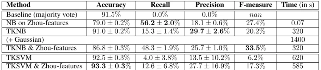
- implementation of Joachims [Joachims, 1999]. To show the competitiveness of our approach, we compared the run- time of our approach with the runtime of the tree kernel implementation of Moschitti. The runtime presented in Ta- ble 1 is measured for a ten-fold cross-validation over the complete dataset. Table 2 contains measured values for a five-fold cross-validation on a 10% sample of the dataset.

Although, the tree kernel na¨ıve Bayes approach is faster the true gain in case of runtime can not be evaluated because our approach is implemented in Java and the SV M

is implemented in C.

6.1 Syskill and Webert Web Page Ratings The first dataset Syskill and Webert Web Page Ratings (SW) is available at the UCI machine learning repository [Frank and Asuncion, 2011]. The dataset originally was used to

1

http://disi.unitn.it/moschitti/

Tree-Kernel.htm

learn user preferences. It contains websites of four do- mains, and user ratings on the particular websites are given.

We will just focus on the classification of the four do- mains. We parsed the websites for the construction of a tree-structured attribute value for each website by using a html-parser

. Unfortunately, the leafs of the resulting html- tree contain huge text fragments in some extent. We con- verted every leaf which contains text into a leaf containing just the word ’leaf ’ have only structured information. Un- fortunately, the trees still were too huge to be processed by the tree kernel implementation of Moschitti which is re- stricted to smaller trees in the origin implementation. An analysis of the trees showed that many equally shaped sub- trees are contained many times in the trees. We pruned the trees by a very trivial heuristic which just deletes equally shaped subtrees in the trees. A tree which is processed in this way just contains unique subtrees. Using this heuris- tic shortens the trees making them applicable by the tree kernel implementation of Moschitti.

To compare our approach to traditional na¨ıve Bayes clas- sifiers we converted the string representation

of the trees into its BOW representation containing the corresponding TF-IDF values. We split the string representation by us- ing spaces and brackets for splitting. In addition, we used the two-grams of this splitted representation as features.

This preprocessing finally resulted in 445 attributes includ- ing the tree containing attribute. The dataset contains 341 examples of four classes. 136 examples belong to class BioMedical, 61 to class Bands, 64 to class Goats and fi- nally, 70 examples belong to class Sheep.

We made a grid-parameter-optimization just by using the tree containing attribute to analyze the best parameter- setting for the tree kernel na¨ıve Bayes approach. We used all seven possible normalization methods. We used σ- values of 0 and 1. We used 21 different λ-values between 0.1 and 10

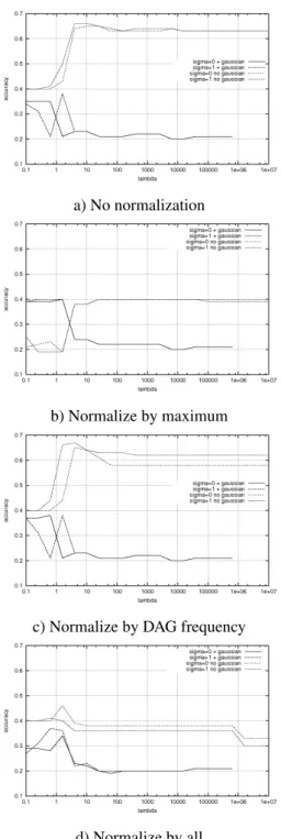
, and in half of the settings we handled the ker- nel values like numerical values expecting a Gaussian nor- mal distribution. On the other half of the settings we ex- pected no gaussian normal distribution and used the (nor- malized) values directly. This setup results in 588 individ- ual experiment-settings. Each of this setting is evaluated by a ten-fold cross validation. Figure 4 shows the visual- ization of four of the seven normalization methods. The plots of the missing normalizations are comparable to the plots of Figure 4 a) and c) and they are missing because of space limitations.

The original tree kernel is restricted to λ-values of 0 <

λ ≤ 1. But for the tree kernel na¨ıve Bayes approach λ- values greater than 1 are delivering the best results. An- other interesting fact is that using the kernel values directly as probabilities – without expecting a normal Gaussian dis- tribution and without normalization – nearly delivers the best results. This is remarkable because expecting a nor- mal Gaussian distribution means to calculate the mean and standard deviation after the construction of the DAGs. Not calculating the mean and standard deviation for the train- ing set results in a more ordinary calculation and finally a better runtime (see Table ??).

It is remarkable that using tree kernel values like numer- ical attributes by expecting a Gaussian normal distribution

2

http://htmlparser.sourceforge.net

3

The string representation of the tree shown in Figure 1 is:

(ROOT (S (NP (NNP John)) (VP (VBD went) (PP (TO to) (NP

(NNP New) (NNP York))) (S (VP (TO to) (VP (VB visit) (NP (NP

(DT the) (NN statue)) (PP (IN of) (NP (NN liberty)))))))) (. .)))

a) No normalization

b) Normalize by maximum

c) Normalize by DAG frequency

d) Normalize by all

Figure 4: Optimization experiments for SW

achieves the worst performance. A reason for this could be outliers contained in the training data. If a tree-structured value contained in the training data delivers a huge tree ker- nel output the mean and standard deviation might not be correct for later use. Unfortunately, finding outliers in tree- structured attributes is not trivial as first of all, the DAGs have to be constructed. After that all kernel-values have to be calculated. If there are any outliers found, they have to be removed from the DAGs, or the DAGs have to be recon- structed. This is a topic for future work. Another argument for outliers to be contained in the training data is visible in Figure 4 b) and d). It delivers bad results to normalize the tree kernel outcome using the maximum and the sum of the kernel outcomes of the training phase. Outliers could create huge kernel-outcomes which cannot be used for nor-

malization during prediction. We extracted the best param- eter setting for the tree kernel na¨ıve Bayes approach using the tree and the BOW features together, too. After that we used the best settings to evaluate the performance of our ap- proach. Table 1 shows the performances (and the standard deviation) concerning accuracy, recall and precision. Those values have been evaluated using a loop of 100 ten-fold cross-validations for the na¨ıve Bayes and tree kernel na¨ıve Bayes approaches. The tree kernel SVM just were evalu- ated on a ten-fold cross-validation. The results presented for the tree kernel SVM are not statistically significant be- cause we just made one ten-fold cross-validation. But the results show that our na¨ıve Bayes tree kernel approach de- livers comparable performance in combination with much shorter runtime, at least.

Using an analysis of variance (ANOVA) test it becomes apparent that using the tree kernel na¨ıve Bayes approach on tree-structured values delivers significantly better results in cases of accuracy and precision than a na¨ıve Bayes ap- proach using no tree-structured values. Using the tree ker- nel na¨ıve Bayes approach on tree-structured and BOW fea- tures delivers slightly better results in cases of accuracy, again.

6.2 SQL

[Bockermann et al., 2009] presented a dataset for intrusion detection. The dataset contains SQL-requests which are parsed to get tree-structured values. The requests are clas- sified as normal request and attack. The relevant class in this binary dataset is relatively rare. The dataset is con- taining just 15 attacks on 1000 requests. Again, we used the tree-structured attribute and the one- and two-grams of the string representation of the trees resulting in 1695 at- tributes. [Bockermann et al., 2009] used an SVM with a tree kernel to detect the attacks. To optimize the parameters for our tree kernel na¨ıve Bayes approach, we used the same setting as already described for the SW dataset. The best performance is achieved by using no normalization and some other normalizations achieving 99.2% accuracy. A default learner which just predicts the majority class would achieve 98.5% accuracy. Like for the Syskill and Webert Web Page Ratings dataset the normalization methods using the sum or the maximum of the outcome been seen during training are not flexible enough, to achieve good results.

They never perform better than the default learner. The re- maining normalization methods do not perform better than no normalization. Additionally, the results and the runtime are bad if we are expecting a Gaussian normal distribution on the values calculated on the training set and using this for calculation of the probabilities during prediction.

Table 1 shows the results using the best parameter set-

ting. Using the tree kernel na¨ıve Bayes approach com-

pared to a na¨ıve Bayes approach using no tree-structured

values delivers significantly better results in cases of preci-

sion and accuracy. All experiments using na¨ıve Bayes ap-

proaches were evaluated using a loop of 100 ten-fold cross-

validations and calculating the average. The results of the

tree kernel SVM are of one ten-fold cross-validation. An

interesting fact is that using a tree kernel SVM on the tree-

structured values and BOW ends up in shorter runtime than

using a tree kernel SVM alone. We suggest that the com-

bination of tree and BOW features results in faster conver-

gence, internally. Using our approach on this dataset deliv-

ers better results for all performance measures compared to

using a SVM. Especially, the shorter runtime is remarkable.

Method Accuracy Recall Precision Time (in s) SW

Baseline (majority vote) 39.9% 25.0% 10.0%

Na¨ıve Bayes on BOW 60.9 ± 1.5% 63.3 ± 1.0% 64.2 ± 0.9% 0.2

Tree Kernel Na¨ıve Bayes 66.5 ± 0.8% 63.0 ± 0.8% 70.8 ± 1.3% 1.81

(+ Gaussian) 2.73

Tree Kernel Na¨ıve Bayes & BOW 66.7 ± 0.8% 64.2 ± 0.8% 67.2 ± 1.4% 1.98

Tree Kernel SVM 60.4 ± 5.8% 55.7 ± 5.5% 59.1 ± 11.7% 34

Tree Kernel SVM & BOW 71.5 ± 7.3% 66.7 ± 8.3% 72.2 ± 14.0% 51 SQL

Baseline (majority vote) 98.5% 50.0% 49.3%

Na¨ıve Bayes on BOW 96.6 ± 0.2% 81.0 ± 2.2% 62.3 ± 1.0% 3.12 Tree Kernel Na¨ıve Bayes 99.3 ± 0.1% 79.6 ± 1.2% 94.3 ± 1.9% 72.2

(+ Gaussian) 612

Tree Kernel Na¨ıve Bayes & BOW 96.6 ± 0.2% 64.9 ± 4.4% 25.1 ± 1.9% 74.7

Tree Kernel SVM 98.5 ± 0.5% 50.0 ± 0.0% 49.3 ± 0.3% 138

Tree Kernel SVM & BOW 98.8 ± 0.8% 62.5 ± 20.2% 64.4 ± 23.2% 110 Table 1: Results of various machine learning approaches on SW and SQL

Combining the tree-structured values with the BOW fea- tures using our tree kernel na¨ıve Bayes approach delivers results which are worse than using the BOW or the tree- structured features exclusively. Developing a smoother combination of both probability distributions inside of the na¨ıve Bayes classifier might overcome this problem.

6.3 ACE 2004

The shared task of the Automatic Content Extraction con- ference 2004 offered one of the first tasks for relational learning [Lin, 2004]. The dataset contains seven types of relations and one irrelevant (negative) class. The dataset consists of more than 50000 examples of which less than 10% belong to one of the seven relation types. Because of the long runtime seen in Table 2 we extracted a sample of 10% of the dataset to evaluate the best parameter setting.

We evaluated the best experiment setting and the perfor- mance of the tested methods on that sample like we did for the SW and SQL datasets. To calculate the values for preci- sion and recall, we calculated the average values of the cer- tain values for each of the seven (positive) classes. These seven classes are the relevant ones. The values for precision and recall for the negative examples are good just because of the amount of negative examples. The performance val- ues of the na¨ıve Bayes approaches are evaluated using a loop of 100 five-fold cross-validations. [Zhou et al., 2005]

presented many features which can be extracted out of tree- structured values for relational learning. These features are nominal or numerical ones and can be used by machine learning methods which cannot handle tree-structured val- ues. We used the features presented by [Zhou et al., 2005]

in several settings shown in Table 2. Again, the tree kernel SVM is a little bit faster if it is applied on a tree-structured attribute together with non-tree-structured attributes. Nev- ertheless, the tree kernel SVM is much slower than our tree kernel na¨ıve Bayes approach. Although, the results for the tree kernel SVM are not significant the results achieved by the tree kernel na¨ıve Bayes approach are comparable. Us- ing the tree-structured attributes in contrast to just using the features presented by [Zhou et al., 2005] (Zhou-features) results in significantly better results in cases of precision and accuracy. In contrast to the other two datasets we eval- uated the f-score, too. The f-score is the harmonic mean of

precision and recall and the best result is achieved by the tree kernel na¨ıve Bayes approach together with the Zhou- features.

7 Conclusion and future work

We presented the novel tree kernel na¨ıve Bayes approach which is a na¨ıve Bayes classifier being able to process tree- structured attribute-values. We present the possibilities in handling these attribute values which are absolutely dif- ferent from traditional attribute value types (nominal and numerical) handled by na¨ıve Bayes classifiers. To memo- rize the training data we are using directed acyclic graphs which efficiently store the trees apparent in the training set for each class. Different types of handling the tree kernel values are analyzed. Exhaustive experiments on three real- world datasets show that our tree kernel na¨ıve Bayes ap- proach delivers good results, although it is a lazy learning method which is not optimized. We have shown that our tree kernel approach can be an efficient and fast alterna- tive to tree kernels embedded in kernel machines. Possible future work is the detection of outliers in tree-structured at- tribute values. In addition, the creation of the DAGs could be done more efficiently. Furthermore, the DAGs are still very complex for special datasets. The question arises if it is possible to just use the relevant pieces of a tree for the creation of the DAGs. For the SQL dataset the combina- tion of tree-structured values and the BOW features deliver worse results. Another topic for future work could be to combine the probability values delivered by tree-structured and flat features even smoother.

Acknowledgements

This work has been supported by the DFG, Collaborative Research Center SFB876, project A1.

References

[Aiolli et al., 2007] Fabio Aiolli, Giovanni Da San Mar- tino, Alessandro Sperduti, and Alessandro Moschitti.

Efficient kernel-based learning for trees. In Computa- tional Intelligence and Data Mining, 2007. CIDM 2007.

IEEE Symposium on, pages 308 –315, 2007.

Method Accuracy Recall Precision F-measure Time (in s)

Baseline (majority vote) 91.5% 0.0% 0.0% nan

NB on Zhou-features 79.0 ± 0.2% 56.2 ± 2.0% 18.1 ± 0.6% 27.4% 0.07

TKNB 91.0 ± 0.2% 15.3 ± 1.4% 29.7 ± 2.6% 20.2% 320

(+ Gaussian) 1400

TKNB & Zhou-features 86.8 ± 0.3% 48.3 ± 1.9% 25.7 ± 1.0% 33.5% 320

TKSVM 92.5 ± 0.3% 4.0 ± 3.8% 13.5 ± 10.2% 6.2% 620

TKSVM & Zhou-features 93.3 ± 0.3% 12.6 ± 6.8% 27.7 ± 16.9% 17.3% 585

Table 2: Results of various approaches on ACE (the runtime values are rounded (NB = Na¨ıve Bayes, TKNB = Tree Kernel na¨ıve Bayes, TKSVM = Tree Kernel SVM))

[Bloehdorn and Moschitti, 2007] Stephan Bloehdorn and Alessandro Moschitti. Exploiting structure and seman- tics for expressive text kernels. In Proceedings of the Conference on Information Knowledge and Manage- ment, 2007.

[Bockermann et al., 2009] Christian Bockermann, Martin Apel, and Michael Meier. Learning sql for database in- trusion detection using context-sensitive modelling. In Proceedings of the 6th Detection of Intrusions and Mal- ware, and Vulnerability Assessment, pages 196 – 205.

Springer, 2009.

[Collins and Duffy, 2001] Michael Collins and Nigel Duffy. Convolution kernels for natural language. In Proceedings of Neural Information Processing Systems, NIPS 2001, 2001.

[Domingos and Pazzani, 1996] Pedro Domingos and Michael Pazzani. Beyond independence: Conditions for the optimality of the simple bayesian classifier. In Machine Learning, pages 105–112. Morgan Kaufmann, 1996.

[Frank and Asuncion, 2011] A. Frank and A. Asuncion.

UCI machine learning repository, 2011.

[Fricke et al., 2010] Peter Fricke, Felix Jungermann, Katharina Morik, Nico Piatkowski, Olaf Spinczyk, and Marco Stolpe. Towards adjusting mobile devices to user’s behaviour. In Proceedings of the Interna- tional Workshop on Mining Ubiquitous and Social Environments (MUSE 2010), pages 7 – 22, 2010.

[Hastie et al., 2003] T. Hastie, R. Tibshirani, and J. H.

Friedman. The Elements of Statistical Learning.

Springer, corrected edition, July 2003.

[Haussler, 1999] David Haussler. Convolution kernels on discrete structures. Technical report, University of Cali- fornia at Santa Cruz, Department of Computer Science, Santa Cruz, CA 95064, USA, July 1999.

[Huang et al., 2003] Jin Huang, Jingjing Lu, and Lambda Charles X. Ling. Comparing naive bayes, decision trees, and svm with auc and accuracy. In in: Third IEEE In- ternational Conference on Data Mining, ICDM 2003, pages 553–556. IEEE Computer Society, 2003.

[Jiang et al., 2010] Peng Jiang, Chunxia Zhang, Hongping Fu, Zhendong Niu, and Qing Yang. An approach based on tree kernels for opinion mining of online product re- views. In Proceedings of the IEEE International Con- ference on Data Mining, pages 256 – 265. IEEE, 2010.

[Joachims, 1999] T. Joachims. Making Large-Scale SVM Learning Practical. In B. Scholkopf, C. Burges, and A. Smola, editors, Advances in Kernel Methods – Sup-

port Vector Learning, pages 169 – 184. MIT Press, Cam- bridge, 1999.

[Lin, 2004] Linguistic Data Consortium. The ACE 2004 Evaluation Plan, 2004.

[Mierswa et al., 2006] Ingo Mierswa, Michael Wurst, Ralf Klinkenberg, Martin Scholz, and Timm Euler. YALE:

Rapid Prototyping for Complex Data Mining Tasks. In Tina Eliassi-Rad, Lyle H. Ungar, Mark Craven, and Dimitrios Gunopulos, editors, Proceedings of the 12th ACM SIGKDD International Conference on Knowledge Discovery and Data Mining (KDD 2006), pages 935–

940, New York, USA, 2006. ACM Press.

[Morik et al., 2010] Katharina Morik, Felix Jungermann, Nico Piatkowski, and Michael Engel. Enhancing ubiq- uitous systems through system call mining. In Proceed- ings of the ICDM 2010 Workshop on Large-scale Ana- lytics for Complex Instrumented Systems (LACIS 2010), 2010.

[Moschitti and Basili, 2006] Alessandro Moschitti and Roberto Basili. A tree kernel approach to question and answer classification in question answering systems. In Proceedings of the Conference on Language Resources and Evaluation, 2006.

[Nguyen et al., 2009] Truc-Vien Nguyen, Alessandro Moschitti, and Giuseppe Riccardi. Convolution kernels on constituent, dependency and sequential structures for relation extraction. In Proceedings of the Conference on Empirical Methods in Natural Language Processing, pages 1378 – 1387. ACL, August 2009.

[Vishwanathan and Smola, 2002] S. V. N. Vishwanathan and Alexander J. Smola. Fast kernels for string and tree matching. In NIPS, pages 569–576, 2002.

[Zhang et al., 2006] Min Zhang, Jie Zhang, Jian Su, and Guodong Zhou. A composite kernel to extract relations between entities with both flat and structured features. In Proceedings 44th Annual Meeting of ACL, pages 825–

832, 2006.

[Zhou et al., 2005] GuoDong Zhou, Jian Su, Jie Zhang, and Min Zhang. Exploring various knowledge in rela- tion extraction. In Proceedings of the 43rd Annual Meet- ing of the ACL, pages 427–434, Ann Arbor, June 2005.

Association for Computational Linguistics.

[Zhou et al., 2007] GuoDong Zhou, Min Zhang,

Dong Hong Ji, and QiaoMing Zhu. Tree kernel-based

relation extraction with context-sensitive structured

parse tree information. In Proceedings of the 2007 Joint

Conference on Empirical Methods in Natural Language

Processing and Computational Natural Language

Learning. Association for Computational Linguistics,

2007.