Research Collection
Report
Model scale standard fire experiments on solid timber panels – Charring and mass loss investigation to determine the variability of the charring rate
Author(s):
Fahrni, Reto; Frangi, Andrea Publication Date:
2021-03
Permanent Link:
https://doi.org/10.3929/ethz-b-000473150
Rights / License:
Creative Commons Attribution-ShareAlike 4.0 International
This page was generated automatically upon download from the ETH Zurich Research Collection. For more information please consult the Terms of use.
ETH Library
Report 2021-02
R. Fahrni, A. Frangi
Model scale standard fire experiments on solid timber panels – Charring and mass loss investigation to
determine the variability of the charring rate
Institute of Structural Engineering
Timber Structures
KEYWORDS: timber structures, fire resistance, testing, experiment, solid timber, charring rate, charring depth, charring, mass loss, scatter, 3D scan, standard fire Reto Fahrni, Andrea Frangi:
Model scale standard fire experiments on solid timber panels – Charring and mass loss investigation to determine the variability of the charring rate
Report 2021-02, March 2021 DOI: 10.3929/ethz-b-000473150
© 2021 Institute of Structural Engineering – Timber Structures, ETH Zurich Citation:
Fahrni, R. and Frangi, A. Model scale standard fire experiments on solid timber
panels – Charring and mass loss investigation to determine the variability of the
charring rate. Report 2021-02, Institute of Structural Engineering – Timber
Structures, ETH Zurich, Zurich, 2021.
Report 2021-02
Model scale standard fire experiments on solid timber panels – Charring and mass loss investigation
to determine the variability of the charring rate
Reto Fahrni
Prof. Dr. Andrea Frangi
Institute of Structural Engineering Timber Structures
ETH Zurich
March 2021
i
Preface
For the design of structures, codes such as the Eurocode guarantee the required structural safety, both for the permanent and the fire design. In timber construction, the fire resistance is usually verified with the standard fire curve, since Eurocode provides simple and accurate design models for this exposure. The current Eurocode for timber in fire (EN 1995-1-2:2004) has evolved historically and uses the 20% fractile value for the strength in case of fire instead of the typical 5% fractile value. This has recently been questioned. In a project funded by the Swiss National Science Foundation (SNF) through the COST Action FP1404 (Fahrni 2021), the current code format was investigated by means of reliability-based code calibrations.
The uncertainty of the charring process is of high importance when it comes to the reliability of a structure. However, literature did not provide sufficient or sufficiently sound data to allow for a probabilistic modeling of the charring process of a structure. This knowledge gap could be overcome with the small experimental campaign of fire resistance tests on solid timber panels presented herein. Since the fire experiments were basic, they provide data that may be used beyond the derivation of a reliability model. Therefore, not only the spatial charring depth, but also temperatures and the mass loss were recorded. Finally, it was decided to publish the data open access.
Zurich, March 2021 Andrea Frangi
iii
Abstract
In a reliability analysis for timber in fire, the uncertainty of the charring rate has an important impact.
The aim of the four solid timber panel fire resistance experiments described herein was to provide reliable data for the probabilistic modeling of the charring process of timber under standard fire conditions. The main interest was on the conjectured fire duration dependency of the charring rate scattering. Therefore four experiments with fire durations of 30/60/90/120 minutes were conducted. The char coal on each specimen was then removed and the remaining specimen was scanned in 3D. The high resolution of the scan allowed to analyze the spatial scattering of the charring rate. As the density of the boards in the specimen was sorted and known, it is possible to analyze also the density dependency of the charring process. The specimens were moreover instrumented with three thermocouples at various depths and the mass loss was recorded as well. The report explains the setup of the experiment as well as how the charring depths were analyzed based on the 3D model. The data is published open access.
v
Zusammenfassung
In Zuverlässigkeitsanalysen für Holzstrukturen im Brandfall spielt die Streuung der Abbrandrate von Holz eine entscheidende Rolle. Die vier hier präsentierten Standardbrandversuche dienten als Datengrundlage für die probabilistische Modellierung von Holz im Brandfall. Hauptsächlich ging es darum die Abhängigkeit der Streuung des Abbrandes/der Abbrandrate von der Branddauer zu untersuchen. Daher wurden vier Versuche mit Branddauern von 30/60/90/120 Minuten durchgeführt. Nach dem Versuch, wurde die Kohle von den Versuchskörpern entfernt und der übriggebliebene Versuchskörper mittels 3D-Scanning aufgenommen. Dank der hohen Auflösung des damit generierten 3D Modells konnte die Streuung räumlich analysiert werden. Da die Bretter in den Versuchskörpern nach der Dichte sortiert waren erlauben es die Ergebnisse die Korrelation zwischen Dichte und Abbrand zu analysieren. Während dem Versuch wurden die Temperaturen in verschiedenen Tiefen an jeweils drei Positionen gemessen. Zusätzlich wurde der Probekörper vor und nach dem Versuch gewogen, um den Masseverlust zu berechnen. Dieser Report beschreibt den Versuchsaufbau und die Auswertung der Abbrandtiefen. Die Rohdaten sind frei zugänglich.
Contents
Preface i
Abstract iii
Zusammenfassung v
1 Introduction 1
1.1 Context . . . . 1
1.2 Uncertainty of the timber charring depth . . . . 2
2 Specimen 3 2.1 Basic properties . . . . 3
2.2 Material . . . . 3
2.3 Installation of thermocouples . . . . 4
2.4 Assembly . . . . 4
3 Fire experiments 8 3.1 Facility . . . . 8
3.2 Installation on the furnace . . . . 8
3.3 Experiment procedure . . . . 9
4 Postprocessing 13 5 Analysis and results 15 5.1 Temperatures . . . 15
5.2 Charring depths and rates . . . 18
5.3 Mass loss rate per unit area . . . 24
6 Outlook 25 References 26 A Equipment 27 A.1 Crane scale . . . 27
A.2 Temperature recording . . . 27
A.3 Furnace . . . 28
Chapter 1
Introduction
1.1 Context
Construction codes guarantee a satisfying safety level by the definition of partial factors and fractile values on uncertain or scattering parameters, respectively. For the accidental design situation ’fire’, the Eurocode 5 (EN 1995-1-2:2004) provides calculation methods that are applicable together with requirements set in (national) fire regulations. Requirements in terms of the fire resistance time (EN<1363-1:2012, ISO 834-1) are used for most constructions. Thereby the structure must resist the standard fire exposure for the given duration.
For timber in fire, the current design approach in Eurocode 5 uses the 20% fractile value for the strength together with the respective partial factorγM,f i= 1. While the latter is identical for steel and concrete structures, the fractile value for the strength for those materials is defined by the 5% fractile, as it is also the case for the ultimate limit state (i.e. not in fire) for any material. The use of 20% fractiles results in a lower safety level compared to 5% fractiles, as the cross sections can be reduced. This also brings an economic advantage for timber compared to the other materials. Thus the use of 20% fractiles was questioned by steel and concrete representatives, which lead to the ETH Zurich research project
‘Reliability based design of timber in fire’, funded by COST, respectively the swiss national funds (SNF), within the COST action FP1404.
The reason for the use of the 20% fractile is found in the calibration of the Eurocode 5 fire part (EN 1995-1-2:2004), where the partial factors of the newly introduced load and resistance factor design (LRFD, Hansell 1978, Ferry Borges 1976) code formats were calibrated towards the antecedent codes, so that the resulting designs were the same (König 2005). To achieve this, a partial factor below unity would have been required, which would be somehow contradictory, as a safety index below unity commonly stands for insufficient safety. For this reason and to be in line with the other materials, it was chosen to set the partial factor toγM,f i= 1, but instead use the 20% fractile value, which had the same effect as a partial factor below unity.
The aforementioned research project aims at proving the current approach in Eurocode 5 and/or to propose changes for the next version of the Eurocode 5. For the first time, reliability analysis is applied to investigate the safety of timber in fire. In a reliability analysis, the uncertain parameters are modeled probabilistically in order to calculate the probability of failure of a structure. For loads and the resistance, models and values for the probability distributions can be found in literature, however not for the charring of timber.
1
2 Chapter 1. Introduction
1.2 Uncertainty of the timber charring depth
The resistance of a timber element in fire is governed by the charring process on the exposed surface and thus the reduction of the remaining sound cross section. The charring process in codes is often modeled by a constant charring rateβ, which is then multiplied by the fire resistance, i.e. the time exposed to standard fire, to get the total charring depth. In reality, the charring rate is maximum at 10 to 20 min and then slightly decreases over time (e.g. Werther 2016). The charring rate depends on the density, among others. Thanks to the high amount of measurements, Fahrni et al. 2017 could show that the correlation is significant, but also that the density dependent variation is low compared to the density-independent scattering. From the result in Fahrni et al. 2017, the uncertainty on the total charring depth for experiments of around 60 min could be determined. However it is unclear how this uncertainty would have to be applied with other fire resistances. Two extremes are conceivable:
1. The uncertainty is applied on the charring rate, i.e. Xβ=logN(µβ, σβ) and the total charred depth isdchar=t·Xβ. The resulting standard deviation ofdchar thus linearly increases with the timet. The coefficient of variation (COV) of the charring depth stays constant. This would mean that the charred surface of a specimen must be smoother for shorter experiments and hillier for longer ones.
2. The uncertainty is applied on the total charring depth: dchar=t·β+Xd whereXd =logN(0, σd).
That means the charred surface is expected to show a similar scatter for any fire duration. The COV of the charring depth thus decreases with the time.
This document presents fire resistance experiments providing the evidence for the development of a probabilistic charring model. Two main questions shall be answered with these experiments: (1) The uncertainty of the charring rate in general and (2) its dependency on the duration of the fire. The first question can be answered with an analysis of the locally varying char depth on a specimen, while the latter is answered by analyzing experiments of different duration. As the local density of the specimen is known, conclusions about the density dependency are possible as well. Finally, the experiments provide data about the mass loss rate of timber exposed to standard fire, which is of interest as a reference when it comes to adhesive testing in fire (Klippel et al. 2018).
Chapter 2
Specimen
2.1 Basic properties
The experiment series consisted of four solid timber panels (STP) of (l x b x h) 961 x 158 x 770 mm. The exposures followed the typical steps of required fire resistances: 30, 60, 90, 120 min (Table 2.1).
2.2 Material
105 spruce (picea abies, Karst) boards of (l x b x h) 960 mm x 160 mm x 60 mm were ordered from sz proholz AG. The timber arrived on 27.2.2019 at 14.6% RH on average (26 arbitrary measurements:
13.0-16.3%, see Fahrni and Frangi 2021). As the boards were chamfered, 2 mm on the exposed side were cut away to create a flat surface. The boards were then (l x b x h) 960 mm x 158 mm x 60 mm. Some of the boards included fingerjoints.
All boards were numbered consecutively. The weight of every board was measured and the density calculated (Fahrni and Frangi 2021). In total 7 specimens shall be created with the timber, of which specimens 1 to 4 were used in this series, being specimen STP 30 to STP 120. Each specimen consisted of 13 boards, i.e. 105−7∗13 = 14 boards were not used in any specimen (specimen 0 in the data), which reduced the range of densities from 373-581 kg/m3to 392-489 kg/m3. Within this range, the boards for each specimen were chosen so that they represented the full range of densities and that the mean densities of the four specimens were all similar (Table 2.1). (Note: The densities given are the mean densities over all boards in the specimen.)
The boards were conditioned to 12% equilibrium moisture content in a climate room (20°C and 65%
RH). The timber boards were stored so that most of the surfaces were exposed to the air. After three month in the climate room, the boards were expected to have reached equilibrium moisture content.
However, the moisture measurements still showed around 14% before the experiments.
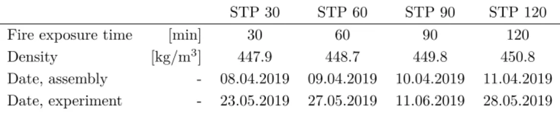
Tab. 2.1: Overview of specimens
STP 30 STP 60 STP 90 STP 120
Fire exposure time [min] 30 60 90 120
Density [kg/m3] 447.9 448.7 449.8 450.8
Date, assembly - 08.04.2019 09.04.2019 10.04.2019 11.04.2019 Date, experiment - 23.05.2019 27.05.2019 11.06.2019 28.05.2019
3
4 Chapter 2. Specimen
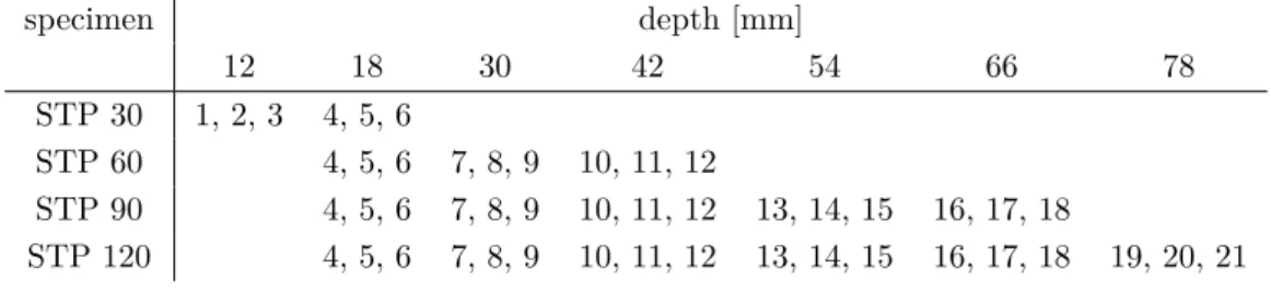
Tab. 2.2: Channel numbers for the measurements at the different depths. Within the same depth, the channel number increases with the distance to the burner. The furnace plate thermometers had channel the numbers 41 to 46.
specimen depth [mm]
12 18 30 42 54 66 78
STP 30 1, 2, 3 4, 5, 6
STP 60 4, 5, 6 7, 8, 9 10, 11, 12
STP 90 4, 5, 6 7, 8, 9 10, 11, 12 13, 14, 15 16, 17, 18
STP 120 4, 5, 6 7, 8, 9 10, 11, 12 13, 14, 15 16, 17, 18 19, 20, 21
2.3 Installation of thermocouples
Thermocouples (TCs) were installed in the center board and were organized in three measurement stations.
The stations were equally spaced along the board, i.e. at 240 mm, 480 mm and 720 mm. Each station had thermocouples installed in the same depths behind the exposed surface. The depths (i.e. the distance to the exposed surface) were chosen based on the fire resistance of the specimen (Table 2.2). Wire TCs (K-w-e-0.5/2.2-in-pa according to Fahrni et al. 2018b) were used. For the product specification see section A.2.
In order to guarantee that the temperature at the measurement point is not influenced by the TC respectively its wire, the first 50 mm of wire next to the measurement should be installed along the isotherms (Fahrni et al. 2018a). Moreover, the spacing between the TCs should prevent mutual interference.
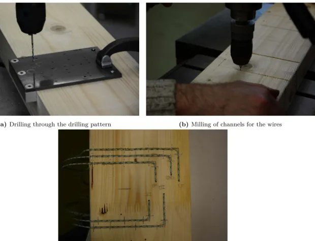
A drilling pattern was used to drill holes with reasonable spacing (Figure 2.1a) from the side of a board to half of its depth (30 mm), where the TCs finally shall be placed. Thus the holes were parallel to the isotherms. To guarantee that the flat gluing surface was not compromised by the TCs, small channels were milled, where the wires could be placed (Figure 2.1b). To ensure that the wires are running at least 50 mm along the isotherms, the milled channels first followed the isotherms for another 20 to 50 mm, before they ran towards the unexposed surface. Finally, the TCs were installed to be in contact with the tip of the drilled hole. The wires were fixed with clips (Figure 2.1c).
2.4 Assembly
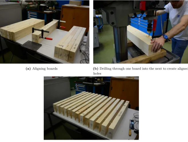
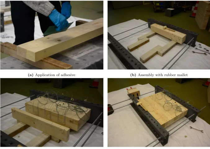
Each specimen was assembled with increasing density from one side to the other (Figure 2.2c). This shall give the chance to investigate the density dependency of the charring rate. The specimen was held together mainly through the application of adhesive (Henkel Loctite/Purbond HB S 709). However, to guarantee a perfectly flat exposed surface, holes were drilled through each perfectly aligned pair of boards (Figures 2.2a and 2.2b). Dowels in those holes guaranteed that the boards kept their position during gluing and pressing (Figure 2.2c). The dowels were positioned close to the unexposed surface (Figure 2.2) and thus did not influence the result of the experiments.
Before gluing, the fire exposed surface was covered with tape, so that pressed out glue would stick on the easily detachable tape and not on the specimen (Figure 2.3a). Glue was always applied on one side of each glueline (Figure 2.3a) using a glue spatula, delivering approximately 175 g/m2. The specimen was then assembled board by board (Figures 2.3b and 2.3c). Each board was forced in place with a rubber mallet. The dowels provided alignment and a first fixation. As soon as all boards were in place, the specimen was pressed between two UPE 300 profiles (Figure 2.3d). The boards were placed on pieces of timber that lifted the specimen so that it was in the center of the steel profile (Figure 2.3b). The force
2.4. Assembly 5
(a)Drilling through the drilling pattern (b)Milling of channels for the wires
(c) Measurement station with installed TCs; the exposed surface is on the right in the picture.
Fig. 2.1: Installation of thermocouples
6 Chapter 2. Specimen
(a)Aligning boards (b)Drilling through one board into the next to create aligned holes
(c) Layup of specimen 2, with inserted alignment-dowels;
before the installation of thermocouples and gluing
Fig. 2.2: Preparation of an aligned specimen with sorted board densities
2.4. Assembly 7
(a)Application of adhesive (b)Assembly with rubber mallet
(c)Instrumented and uninstrumented boards could be han- dled the same
(d)Closed press
Fig. 2.3: Gluing and pressing
was applied through four threaded bars M16 that were manually tightened as much as possible with a 30 cm long wrench.
After one day of pressing, the pressure was released and the tapes on the exposed surface was removed.
The specimens then were put back to the climate chamber until the day of the experiment.
Chapter 3
Fire experiments
3.1 Facility
The experiments were conducted on the horizontal model scale furnace (technical data in section A.3) at the former VKF-ZIP laboratory in Dübendorf, Switzerland (formerly EMPA fire lab). The furnace has a horizontal open area of slightly more than l x b 960 x 800 mm. The two oil burners are controlled by 6 plate thermometers placed approximately 100 mm below the specimen. In the raw data, the plate thermometers have the channel numbers 41 to 46. Due to the heat contribution of the timber specimen, one burner had to be shutdown from time to time. It was alternated between both burners. The (under-) pressure in the furnace was set to -5 Pa, compared to the ambient pressure. The furnace is controlled automatically, except for shutting off of burners and deselecting plate thermometers on failure of them.
The latter happened to channel number 43 in the experiments STP 90 and STP 120.
3.2 Installation on the furnace
The installation on the furnace had to ensure a one-dimensional heat flow, i.e. a one-dimensional charring.
This mainly makes demands on the insulation between the furnace and the specimen. On one hand it must be airtight, since entering air (due to the underpressure) could lead to increased charring along the entering path due to the additional oxygen that flows in. On the other hand, the insulation around the specimen (i.e. on the surfaces parallel to the heat flow) ideally should create an adiabatic surface. Lack of insulation could otherwise lead to decreased charring close to these surfaces due to the cooling from the ambient air, respectively the heat loss perpendicular to the intended charring direction through the deficient insulation.
Finally, the mounting should allow a rapid removing at the end of the experiment to suddenly extinguish and cool the specimen by applying water and to stop the charring process. As the mass loss of the specimen was of interest as well, the remaining mass had to be measured between removing from the furnace and the application of water. Thus the insulation had to be easily removable.
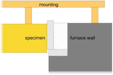
The following installation and insulation procedure fulfilled above aims: Before the specimen was installed, 40 mm thick soft insulation was placed on the ring around the opening (Figure 3.2a). The specimen was then placed hanging on a mounting that transferred the load to three bearings on the furnace walls (Figures 3.1 and 3.2f). The dimensions of the specimen were only slightly smaller than the furnace opening, so that it could reach a few centimeters below the insulation on the ring, without affecting the one-dimensional charring direction despite having no insulation on the side in this area. The upper part
8
3.3. Experiment procedure 9
Fig. 3.1: Mounting of the specimen and placement of the insulation
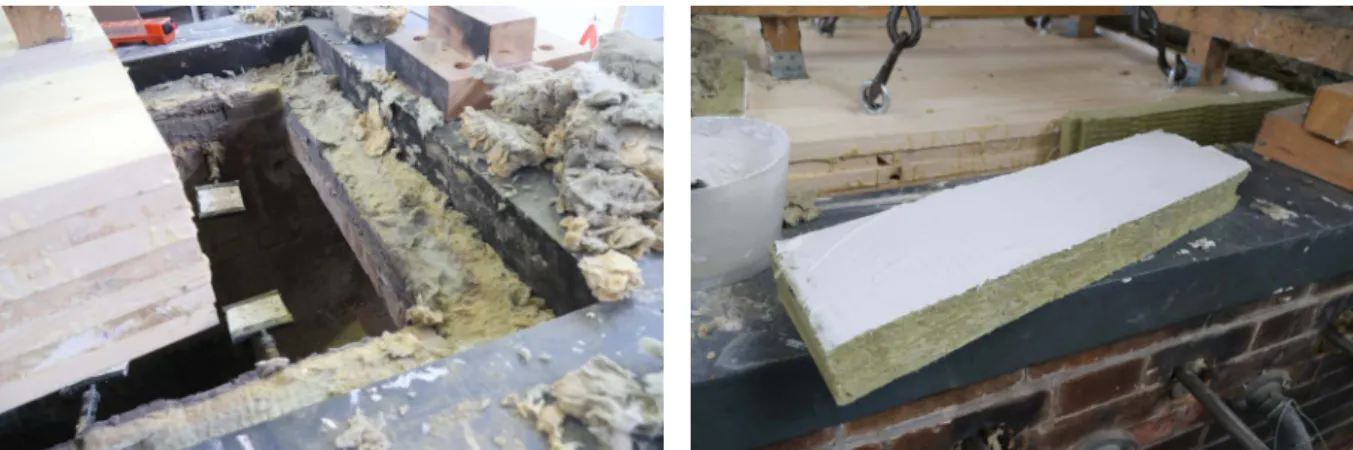
of the sides were then covered with 40 mm thick stiff insulation that was ‘glued’ to the specimen with gypsum (Figure 3.2b). Only a small layer of gypsum was added, so that the insulation sticked well, but without adding a lot of weight to the specimen. The width of the insulation was chosen so that it reaches slightly above the specimen (Figure 3.2c), while being in firm contact with the soft ring insulation to tighten the joint. The length of two insulations on opposite sides had the same length as the specimen, so that the insulation on the remaining two sides could reach beyond the specimen and close the side insulation ring. The corner is critical in terms of insulation and air tightness. Thus, additional gypsum was placed where the two insulations and the edge of the specimen come together (Figure 3.2d). On gluing/pressing the insulation on the specimen, the gypsum spread at the corner and filled any remaining gap. Along the top edge between insulation and the specimen, additional gypsum was added for a better air tightness (Figure 3.2e). Finally the remaining gap between the stiff insulation and the furnace wall was filled with stiff or soft insulation as a further insulation and air tightening measure (Figure 3.2f).
3.3 Experiment procedure
Before the installation, the mass of the specimen was measured with and without the mounting, using a crane scale (technical data in section A.1). After the specimen was positioned and the gaps insulated, the thermocouples were connected to the recording device (technical data in section A.2).
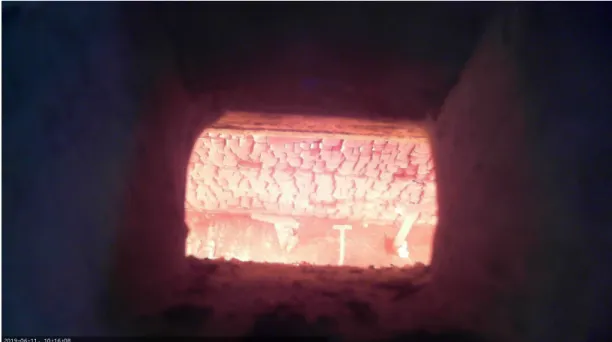
Finally, the proper installation, especially of the thermocouples, was checked again, before the furnace was started. During the whole experiment, a webcam gazed into the furnace through a window of approximately 100x100 mm and recorded a picture every five seconds (Figure 3.3). Nothing surprising was recorded: With increased crack formation, small pieces of char fell off from time to time, but there was no visible char recession (i.e. the specimen thickness including the char coal stayed roughly the same).
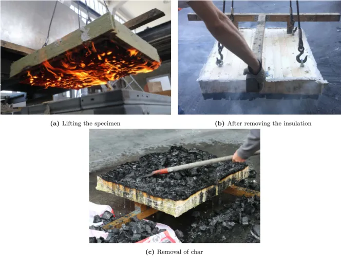
Before the end of the experiment, the crane scale was tared. The thermocouples were cut close to the specimen surface a few seconds before the experiment ended so that the specimen could be removed right at the end. The specimen was lifted with the crane and transported out of the lab. On liftoff, flames came up on the side of the specimen for a few seconds (Figure 3.4a). After ca. 15 s, when the specimen was not over the furnace opening anymore and the flames reduced to appear only locally on the charred surface, which allowed a safe removal of the glued side insulation by a stroke with the fist during transportation (Figure 3.4b). Thereafter, the reading of the crane scale was noted. Finally, the specimen was put on the ground with the charred side on top for extinguishing. It took less than two minutes from the end of the
10 Chapter 3. Fire experiments
(a)Horizontal soft insulation around the furnace opening before mounting the specimen.
(b)Layer of gypsum on stiff insulation, used for airtightness and as adhesive for the insulation. Before gluing on the side of the specimen.
(c)Insulation applied to the specimen. Insulation is of the same length as the specimen and is fixed so that it is pressed slightly into the horizontal insulation below.
(d) Additional gypsum applied to make the critical edge between both insulations and the specimen airtight.
(e)Gypsum along the top edge between the specimen and the side insulation.
(f)Final installation on the furnace. The gap between insu- lation and furnace is filled with any kind of insulation.
Fig. 3.2: Specimen installation and insulation. Pictures from a CLT-specimen from another test series.
3.3. Experiment procedure 11
Fig. 3.3: Recording with the webcam. Few small areas where pieces of char coal fell off can be seen. The dimensions (100x100 mm) of the two plate thermometers on the opposite wall can serve as a scale.
experiment until extinguishing with water. The char coal was then roughly removed (Figure 3.4c), so that the remaining timber would cool faster.
12 Chapter 3. Fire experiments
(a)Lifting the specimen (b)After removing the insulation
(c)Removal of char
Fig. 3.4: After the end of the experiment
Chapter 4
Postprocessing
As the local charring rates were of interest, the remaining geometrical shape of the charred surface had to be determined. Therefore the specimens were 3D-scanned with an optical method, as this probably has the highest accuracy and resolution.
A few days after the experiment, the charred surface of the specimen was further cleaned using a wheel brush on a power drill1. Cleaning with a steel/wheel brush is reliable in terms of the resulting cleaned surface, as long as a minimum pressure is applied and cleaning is not stopped until no further charcoal gets removed.
The 3D scanning was done by taking between 79 and 100 pictures of each specimen from many different views/angles with the same camera, lens and the same focal length. (Important for the method.) There must be a reference length somewhere in the final model. Therefore a meterstick was placed on the specimen. The specimen was mounted vertically so that pictures could be taken from all around, including the backside. To make it easier for the software to find out the viewing angles and position of the camera, timber boards were mounted on the specimen’s sides. An exemplary picture of the setup is shown in Figure 4.1a. Creating a 3D-model of that setup allowed that the remaining local thickness of the specimen could be be determined as the distance between the front and the back of the specimen. Alternatively the specimen could have been placed flat on the ground. However, neither the floor nor the back of the specimen is truly flat so that at least one corner stands up a few millimeters. Thus calculating the remaining thickness between the charred surface and the interpolated floor would introduce an error in the order of a few millimeters.
Using the software Autodesk Recap Photo 20.0.1.5, a colorized 3D model is generated from the pictures.
Thereby the software detects the position and views of all pictures automatically and can derive the 3D model. Figure 4.1b shows the created 3D model of the specimen together with the camera positions. The created model was then scaled accoring to the meterstick and unnecessary parts removed. The coordinate system was centered in the specimen, with the y-direction being along the timber boards, the x-direction pointing to the higher-density end of the buildup and the z-direction towards the charred surface.
The mesh was then imported into MATLAB for further processing. First, the positioning of the coordinate system was improved, as the positioning from the scan-software is not accurate enough. When the coordinate system was aligned appropriately, the remaining height of the specimen could be derived as the z-coordinate difference for the same x and y-coordinates on the top and bottom surface. The bottom was not perfectly flat (especially at the bondlines, due to the chamfering and locally overstanding adhesive). Thus the bottom surface was smoothed by calculating its z-coordinate as the mean over a
1This is an extremely dirty job. Hints: Do this task outdoors, wear safety glasses and a mask and be ready to wash the clothes and yourself afterwards. Manually using a steel brush is less dirty, but also significantly slower.
13
14 Chapter 4. Postprocessing
(a)Exemplary, single picture (b)Location and direction of photos in the created 3D model Fig. 4.1: Scanning of the specimen
square of 10 cm. To avoid any influence from corner roundings along the edges, the outermost 70 mm were neglected in the analysis, i.e. only the inner area of 620 x 820 mm was analyzed. The remaining height was evaluated for a grid with 0.5 mm mesh-size, which resulted in more than two million2evaluated points.
21641*1241=2’036’481 points
Chapter 5
Analysis and results
5.1 Temperatures
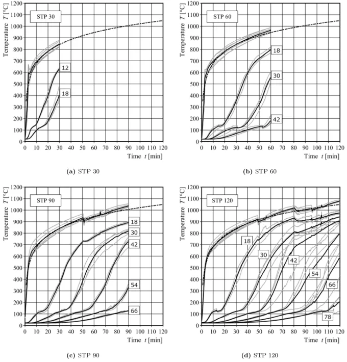
In Figures 5.1 and 5.2 the measured temperatures are plotted over the time. Figure 5.2 shows the mean temperature curves of every specimen in one diagram, while Figure 5.1 shows separate plots for each specimen, including also the single measurement (in grey). In specimen STP 120, a knot was within the center measurement station (Figure 5.3b). Despite the fact, that most temperature measurements were not directly in the knot, it reduced the local charring significantly, which can be seen in the lower temperatures in this station. The effect can also be seen e.g. in Figure 5.7a.
The raw data of the measured temperature can be found in Fahrni and Frangi 2021.
15
16 Chapter 5. Analysis and results
(a)STP 30 (b)STP 60
(c)STP 90 (d)STP 120
Fig. 5.1: Time-temperature plots for each experiment. Single (grey) and mean (black) values over three thermocouple measurements at different depths. Additionally the furnace temperature (mean over 5 (STP 90 and 120) respectively 6 (STP 30 and 60) measurements) and the standard fire curve are shown.
5.1. Temperatures 17
Fig. 5.2: Time-temperature plots of all experiments in one plot. Mean values over three thermocouples measurements at different depths. Additionally the furnace temperature (mean over 5 respectively 6 measurements) and the standard fire curve are shown.
18 Chapter 5. Analysis and results
(a)STP 90
(b)STP 120, many knots around measurement station 2 (center)
Fig. 5.3: Boards with installed thermocouples. Unfortunately there are no pictures of STP 30 and STP 60.
5.2 Charring depths and rates
In Figures 5.4, 5.5, 5.6 and 5.7 the charring depths derived from the 3D model are shown together with a picture of the charred surface. The plot of the charred depth (a) only shows the evaluated area, i.e. not the outer 70 mm. The scale shown in the plots nevertheless starts at the specimens edges and thus in the plots does not start at zero. The charred surface (b) shows the whole specimen’s surface and is roughly scaled the same as the plot. Therefore it appears larger. The orientation in all graphs presented is so that the top was closer to the burners, the bottom was closer to the exhaust and the density increases from left to right.
In Fahrni and Frangi 2021 the remaining heights of the evaluated area can be found for every specimen.
The data has the same orientation as the plots here.
From the charring depth, the charring rate can be calculated by dividing by the fire duration. The resulting plots for all specimens are shown in Figures 5.8 and 5.9. Figure 5.8 uses the same scale for all specimens for a better comparison among the specimens, while Figure 5.9 has separate scales.
5.2. Charring depths and rates 19
(a)Charring depth (b)Surface after char coal removal
Fig. 5.4: STP 30
(a)Charring depth (b)Surface after char coal removal
Fig. 5.5: STP 60
20 Chapter 5. Analysis and results
(a)Charring depth (b)Surface after char coal removal
Fig. 5.6: STP 90
(a)Charring depth (b)Surface after char coal removal
Fig. 5.7: STP 120
5.2. Charring depths and rates 21
(a)STP 30 (b)STP 60
(c)STP 90 (d)STP 120
Fig. 5.8: Charring rates of all specimens with one common color scale
22 Chapter 5. Analysis and results
(a)STP 30 (b)STP 60
(c)STP 90 (d)STP 120
Fig. 5.9: Charring rates of all specimens with separate color scales
The local charring rates were statistically evaluated as well. Table 5.1 shows the mean and standard deviations over all (>2 millions) locally evaluated points. The problem with this analysis is that the points are not independent of each other (i.e. they are correlated), as the surface is locally smooth. Thus two neighboring points (0.5 mm from each other) will differ a little. As two neighboring points are correlated, there must exist a certain distance after which two arbitrary points can be deemed independent: the correlation length.1
1Note: Analyzing the empirical cumulative distribution function shows rather fat tails compared to a fitted normal distribution. From the perspective of the author, the local correlation is the cause for this. Trying to find an appropriate distribution function for the raw, correlated charring depths, a logistic distribution turned out to provide the best fit of all examined distributions, i.e. all distributions available in Matlab. However, a more in depth analysis would be required to
5.2. Charring depths and rates 23
To reduce the effect of the local correlation, it might be appropriate to calculate the mean height over a certain area and then evaluate the scatter among those mean values. When the chosen area is equivalent to the correlation length, then the distribution of the area mean values would eventually be the correct representation of the charring rate uncertainty. However, when the area was chosen larger than the correlation length, the resulting standard deviation would be an underestimation. On the other hand, if the area is chosen smaller than the equivalent correlation length, the resulting standard deviation was larger than the actual one. As the correlation length was not determined so far, the resulting sample statistics are shown for two exemplary areas: Table 5.2 shows the sample mean and standard deviation for an averaged area of 20 by 20 points (10 by 10 mm), Table 5.3 for an area of 100 by 100 points (50 by 50 mm) respectively. The mean value of the charring rate is basically independent of the chosen area. However, as the total analyzed width and height is not necessarily a multiple of the chosen area (width/height), a few points are not considered in the analysis of averaged heights and thus their means
slightly differ from the mean over all points.
As can be seen from the differences in the coefficient of variation (COV) in Tables 5.1, 5.2 and 5.3, the impact of the effect described above is significant. At the same time it shows the importance of describing how the data was obtained and evaluated to allow a correct interpretation at a later stage. The scattering of charring rates/char depths derived with one grid size can usually not be compared with another grid size. Nevertheless, the mean value theoretically is comparable.
Tab. 5.1: Charring rate statistics over all points, i.e. every 0.5 mm STP 30 STP 60 STP 90 STP 120 mean [mm/min] 0.6687 0.6256 0.6060 0.6248 median [mm/min] 0.6723 0.6266 0.6025 0.6145 std [mm/min] 0.0614 0.0516 0.0441 0.0602
COV [-] 9.18 % 8.25 % 7.28 % 9.64 %
Tab. 5.2: Charring rate statistics for the mean charring rate of 20 by 20 points, i.e. 10 by 10 mm STP 30 STP 60 STP 90 STP 120
mean [mm/min] 0.6687 0.6256 0.6059 0.6247 median [mm/min] 0.6722 0.6267 0.6026 0.6145 std [mm/min] 0.0603 0.0508 0.0436 0.0599
COV [-] 9.02 % 8.12 % 7.20 % 9.59 %
Tab. 5.3: Charring rate statistics for the mean charring rate of 100 by 100 points, i.e. 50 by 50 mm STP 30 STP 60 STP 90 STP 120
mean [mm/min] 0.6687 0.6249 0.6040 0.6227 median [mm/min] 0.6728 0.6282 0.5988 0.6095 std [mm/min] 0.0508 0.04 0.0375 0.0549
COV [-] 7.60 % 6.40 % 6.21 % 8.82 %
investigate local correlations and its effect on fitting a distribution over partially correlated samples.
24 Chapter 5. Analysis and results
5.3 Mass loss rate per unit area
From the difference between the specimens mass before and after the experiment, the mass loss can be calculated. By further dividing by the exposed area and the duration of the experiment, the mass loss rate per unit area can be calculated. All results are shown in Table 5.4. It must be noted that the division of the used crane scale was 0.5 kg in the used measurement range (A.1).
The method has some inaccuracies:
• Some smaller parts of the char naturally do fall off during the experiment as well as during handling after the experiment. This is understood as part of the natural scattering when performing experiments with timber.
• It is assumed that both mass measurements are made with the same auxiliary masses attached to the specimen. However, the gypsum from gluing the side insulation cannot completely be removed after the experiment. This leads to an underestimation of the mass loss, which cannot be corrected.
However, it is deemed to be small compared to the natural scatter of the timber.
• The mass difference due to the cut TC cables can be corrected by measuring the weight of the cut cables.
• In the calculation of the mass loss rate per unit area it is assumed that the charring process is perfectly one dimensional. In the present experiments this is a good assumption, since the insulation on the side were very effective in preventing additional charring and/or cooling on the side. However, it can introduce significant uncertainty to the result if the side insulation is not done appropriately.
In the present experiments, these inaccuracies are low compared to the 0.75 kg precision / 0.5 kg division of the crane scale and thus surely can be neglected.
Tab. 5.4: Mass loss, mass loss rate and mean char depth of all specimens. The actual, measured dimensions of the specimen were used to calculate the mass loss rate per unit area.
STP 30 STP 60 STP 90 STP 120
mass loss [kg] 5.5 11 16 22
mass loss rate [kg/m2h] 14.9 14.9 14.4 14.9 mean char depth [mm] 20.06 37.54 54.54 74.98
Chapter 6
Outlook
It is an open question, how the scattering of the char depth respectively the charring rate should be measured and indicated appropriately. The question is likely answerable through the application of advanced statistical methods. Thereby the correlation length could be found. At the same time, this could allow a more advanced probabilistic modeling of the charred surface by random fields. This could give further insights about the possible size dependency of the probability of failure of a timber element in fire.
25
References
EN 1995-1-2:2004 (2004).Eurocode 5: Design of Timber Structures - Part 1-2: General - Structural Fire Design.
EN<1363-1:2012 (2012). Fire Resistance Tests - Part 1: General Requirements; English Version EN 1363-1:2012.
Fahrni, Reto (2021). “Reliability-Based Code Calibration for Timber in Fire”. Dissertation. Zurich: ETH Zurich.
Fahrni, Reto and Andrea Frangi (2021). “Model Scale Standard Fire Experiments on Solid Timber Panels – Charring and Mass Loss Investigation to Determine the Variability of the Charring Rate - Data
Collection”. In: in collab. with Reto Fahrni et al.doi: 10.3929/ETHZ-B-000465255.
Fahrni, Reto et al. (2017). “Fire Tests on Glued Laminated Timber Beams with Specific Local Material Properties”. In:Fire Safety Journal.
Fahrni, Reto et al. (2018a). “Correct Temperature Measurement in Fire Exposed Wood”. In: WCTE.
Seoul, KOR.
Fahrni, Reto et al. (2018b). “Investigation of Different Temperature Measurement Designs and Installations in Timber Members as Low Conductive Material”. In:10th International Conference on Structures in Fire. Structure in Fire. Belfast, UK.
Ferry Borges, Julio (1976).Common Unified Rules for Different Types of Construction and Material. 116-E. Comité euro-international du béton (CEB).
Hansell, W.C. (1978). “Introduction to Eight LRFD Papers”. In:Journal of the Structural division 104.9.
ISO 834-1 (1999).Fire-Resistance Tests - Elements of Building Construction - Part 1: General Require- ments.
Klippel, Michael et al. (2018). “Assessing the Adhesive Performance in CLT Exposed to Fire”. In: WCTE.
Seoul, KOR, BLD–O7–02.
König, Jürgen (2005). “Structural Fire Design According to Eurocode 5—Design Rules and Their Back- ground”. In:Fire and Materials29.3, pp. 147–163.issn: 0308-0501, 1099-1018.doi:10.1002/fam.873. Werther, Norman (2016). “Einflussgrössen auf das Abbrandverhalten von Holzbauteilen und deren
Berücksichtigung in empirischen und numerischen Beurteilungsverfahren”. TU Munich. 181 pp.
26
Appendix A
Equipment
A.1 Crane scale
• Type: Meili MCWN
• Max load: 6000 kg
• Selected measuring range: 0-1500 kg
• Division: 0.5 kg
• Tolerance: 0.75 kg (0.05% of the measuring range max value)
A.2 Temperature recording
Thermocouples:
• Type: K
• Diameter: 2x0.5 mm
• Class: 1
• Manufacturer: mcs laboratory AG, Altdorf, Switzerland
• Test point: welded junction
27
28 Chapter A. Equipment
A.3 Furnace
Fig. A.1: Drawing of the model scale furnace at EMPA (german).