Reference point insensitive molecular data analysis

(1)

...

Reference point insensitive molecular data analysis

M. Altenbuchinger

^1,∗

, T. Rehberg

^1,∗

, H. U. Zacharias

²

, F. Stämmler

^{1, 4}

,

K. Dettmer

²

, D. Weber

³

, A. Hiergeist

⁴

, A. Gessner

⁴

, E. Holler

³

, P. J. Oefner

²

, and R. Spang

¹

1Statistical Bioinformatics, Institute of Functional Genomics, University of Regensburg, Regensburg, Germany

2Institute of Functional Genomics, University of Regensburg, Regensburg, Germany

3Department of Hematology and Oncology, Internal Medicine III, University Medical Center, Regensburg, Germany

4Institute of Clinical Microbiology and Hygiene, University Medical Center, Regensburg, Germany

∗These authors contributed equally to this work.

Abstract

Motivation:

In biomedicine, every molecular measurement is relative to a reference point, like a fixed aliquot of RNA extracted from a tissue, a defined number of blood cells, or a defined volume of biofluid.

Reference points are often chosen for practical reasons. For example, we might want to assess the metabolome of a diseased organ but can only measure metabolites in blood or urine. In this case the observable data only indirectly reflects the disease state. The statistical implications of these discrepancies in reference points have not yet been discussed.

Results:

Here we show that reference point discrepancies compromise the performance of regression models like the LASSO. As an alternative, we suggest zero-sum regression for a reference point insensitive analysis. We show that zero-sum regression is superior to the LASSO in case of a poor choice of reference point both in simulations and in an application that integrates intestinal microbiome analysis with metabolomics. Moreover, we describe a novel coordinate descent based algorithm to fit zero-sum elastic nets.

Availability:

The R-package “zeroSum” can be downloaded at https://github.com/rehbergT/zeroSum.

Moreover, we provide all R-scripts and data used to produce the results of this manuscript as supplementary material.

Contact:

Michael.Altenbuchinger@ukr.de, Thorsten.Rehberg@ukr.de, and Rainer.Spang@ukr.de

Supplementary information:

Supplementary material is available at

Bioinformatics

online.

1 Introduction

The emergence of novel technologies and experimental protocols for molecular and cellular profiling of biological samples is continuously gaining speed for at least one decade and there is no end in sight. Every technology brings new computational challenges in the normalization and interpretation of the data produced. Nevertheless, many of these data types share common computational challenges. For example the high dimensionality of profiles has established machine learning techniques

including penalized regression models (Hoerl and Kennard, 1970;

Tibshirani, 1996; Efronet al., 2004; Hastieet al., 2009) as standard tools of genomic data analysis.

In contrast, little attention has been given to the choice of reference points for measurements. Exemplary reference points include for example one microgram of RNA, all mRNA from 1 million cells, all metabolites in 1 ccm of blood, just to name a few. In a typical biomedical protocol, DNA, RNA or proteins are extracted from specimens such as blood, urine or tissue, and a fixed size aliquot of these molecules is profiled. In intestinal microbiome sequencing, for instance, DNA encoding for 16S rRNA genes 1

journals.permissions@oup.com Associate Editor: Dr. Ziv Bar-Joseph

at Universitaetsbibliothek Regensburg on November 14, 2016http://bioinformatics.oxfordjournals.org/Downloaded from

(2)

are extracted, a fixed size aliquot of DNA is sequenced and the reads are mapped to taxonomic units. Here, the reference point is a fixed size aliquot of DNA.

Also, the difference between profiles relative to two reference points are not always small. For example Linet al.(2012) and Nieet al.(2012) have shown that inducing the expression of the transcription factor MYC causes transcriptional amplification, a global increase in transcription rates of all currently transcribed genes by a factor of two to three, which can only be detected by using the number of cells rather than a fixed amount of RNA as reference point. Similarly in the context of epigenomics, Orlando et al.(2014) report global changes in ChIPseq signals across experimental conditions. Reference points for measurements in tissue specimens like the weight, the volume, or the DNA content can be greatly and differentially affected by the cellular composition of the specimen or even by disease state (Büttner, 1967). In all these instances, changing the reference point changes the data including the correlations between molecular features.

This will affect both statistical analysis and biological interpretation.

Reference points are closely linked to data normalization and preprocessing. Normalization changes the reference point. For example, if we normalize profiles to a common mean, we generate a data internal reference point. In this case the data becomes quasi compositional. If in contrast we normalize to a constant value for one or several housekeeping features we choose another data internal reference point and data that was compositional, looses this property.

Finally, sometimes it might not be possible to generate profiles for the relevant reference point. For instance, one may be interested in the effect that disease exerts on the concentration of metabolites in an organ.

Unless one were to take a biopsy from the organ, such changes can only be determined indirectly by measuring the metabolites in biomedical specimens more readily available, such as blood, urine, feces or breath.

How much of the metabolites in the organ make it into these specimens might differ from patient to patient. In this case the reference point is unknown.

In summary, even with meticulous experimental designs the reference point can remain suboptimal or even obscure. In such cases statistical analysis and biological interpretation should not depend on it. Linet al.

(2014) pioneered zero-sum regression as a tool for feature selection in high-dimensional compositional data. However, zero-sum regression is not limited to compositional data. On the contrary, it provides the framework for a reference point insensitive data analysis.

Extending the work of Linet al.(2014), we here show that zero-sum regression yields reference point insensitive models. We extend zero-sum regression to elastic net models and contribute a fast coordinate descent algorithm to fit zero-sum elastic nets. This algorithm is implemented as an R-package with crucial functions written in C to further reduce computing time. To the best of our knowledge, our tool is the first freely available R-package for reference point insensitive data analysis using zero-sum regression. Finally, we demonstrate the use of a reference point insensitive analysis in an application that integrates intestinal microbiome analysis with metabolomics.

2 A strategy for reference point insensitive data analysis

Let(xi, yi)be data, wherei = 1, . . . , N indicates the measurements andxi = (xi1, . . . , xip)^T the predictor variables. The corresponding responses areyi. We will discuss the regression problem

yi=β0+

∑p j=1

βj(xij+γi) +ϵi, (1)

wherexijis known, but the sample specific shiftsγiare not. In this data the responseyidoes not only depend on the observed data but also on an unobserved confounderγi. We will argue that these confounders are omnipresent in genomic data analysis and that they result from ambiguous reference points. We will then discuss zero-sum regression as an option for reference point insensitive data analysis.

2.1 Proportional reference point insensitivity

Molecular quantifications are always relative to a reference pointr. We say that two reference pointsr1 andr2 are proportional, if changing the reference point fromr1 tor2amounts to rescaling all features in a profile: Letibe a sample. IfZiis a profile ofirelative tor1andXithe corresponding profile relative tor2, thenZi= ΓiXi, whereΓi∈Ris a sample-specific rescaling factor. Omics data is typically log-transformed.

Hence, the change of scale translates into a shift of the log-profiles:

zij=xij+γi, (2)

wherezij, xijandγiare the log-transformed values ofZij,Xij, and Γi, respectively. The shiftsγican vary across samples. If the measured reference point is a fixed size aliquot of molecules, but the reference point of clinical relevance is an organ or an entire patient, theγiare unknown.

They can be seen as latent confounders.

Letxibe a data set measured relative tor1andyiis the respective response. We assume that theyiare conditionally independent. Changing the reference point fromr1tor2yields the regression equation (1). We call a regression modelproportional reference point insensitiveorPRP- insensitive, if the predictionsˆyido not depend on the chosen reference pointr. This is the case if the regression weightsβjsum up to zero,

∑p j=1

βj= 0. (3)

Note that the standard tool kit of linear regression analysis is sensitive to the reference point. This includes penalized methods like ridge regression (Hoerl and Kennard, 1970) or the LASSO (Tibshirani, 1996).

2.2 Zero-Sum-Regression is PRP-insensitive while the LASSO and the Elastic Net are not

The LASSO is a regularized linear regression model that still works for data with more features than samples where least squares estimates are no longer an option. It has the additional appeal that fitted models are sparse in the covariates. Covariates with non-zero coefficients can be interpreted as biologically important. Moreover, predictions can be calculated from only a few covariates. A LASSO model is estimated by minimizing

1 2N

∑N i=1

(

yi−β0−

∑p j=1

βjxij

)2

+λP(β), (4)

with respect to the coefficient vector β = (β1, . . . , βp)^T and the interceptβ0. HereP(β) = ||β||1is a penalty term that implementsa prioripreference for sparse models. The tuning parameterλcalibrates sparseness. If we replace the L1 norm in the log-likelihood (4) by P(β) = α||β||1+ (1−α)/2||β||²2, we have the log-likelihood of the elastic net (Zou and Hastie, 2005). Forα= 1this gives us the LASSO and forα= 0the non-sparse ridge regression.

These models are only PRP-insensitive if the regression coefficients add up to zero. If the profiles are mean centered, the standard least squares estimates forβform a one dimensional subspace that includes the unique zero-sum estimate (see supplemental materials). In other words, from all optimal solutions we can simply choose one that is PRP-insensitive. Also

(3)

ridge regression models automatically meet the zero-sum condition for centered profiles (see supplemental materials). However, as we will see neither the LASSO nor the elastic net do.

Zero-sum regression¹ yields sparse PRP-insensitive models. For compositional high dimensional data, Linet al.(2014) combined the zero-sum condition with theL1 penalty of the LASSO. In their zero- sum regression they minimize the penalized log-likelihood (4) under the constraint (3). Hence, unlike the standard LASSO or the elastic net, zero-sum regression models are always PRP-insensitive. Condition (3) uncouplesyifrom the reference points. Thus, the corresponding zero-sum estimates forβ0andβare also reference point insensitive.

It is instructive to see that zero-sum models are driven by the ratios of features rather then the individual absolute features. In ratios the reference points cancel. For illustration, consider a model with only two features xi1andxi2on log-scale. Then, the sum of squares becomes

∑N i=1

(

yi−β0−β1(xi1−xi2))2

. (5)

Note that the zero-sum constraint turnedxi1−xi2into the only predictor variable. Sincexi1−xi2= log(Xi1/Xi2), it is the ratioXi1/Xi2of the original data that drives the model.

2.3 The Zero-Sum Elastic Net

We next describe an extension of the coordinate descent (CD) algorithm for the elastic net (Friedmanet al.(2007, 2010)) that preserves the zero-sum constraint. The challenge is to solve:

min

(β₀,β)∈R^p+1Rλ(β0,β) = min

(β₀,β)∈R^p+1

[ 1 2N

∑N i=1

(yi−β0

−

∑p j=1

βjxij

)2

+λ (1−α

2 ||β||²2+α||β||¹ ) ]

subject to:

∑p j

βj= 0. (6)

We replaceβs=−∑p j=1 j̸=s

βj, yielding

Rλ(β0,β) = 1 2N

∑N i=1

(

yi−β0−

∑p

j=1 j̸=s

xijβj+xis

∑p

j=1 j̸=s

βj

)2

+λ (1−α

2 (∑^p

j=1 j̸=s

β_j²+(∑^p

j=1 j̸=s

βj

)2)

+α(∑^p

j=1 j̸=s

|βj|+

∑p

j=1 j̸=s

βj)) .

(7)

We start with a standard CD routine of iteratively optimizing the ratio between two coordinatesβsandβkwhile keeping all others constant. To this end, we need all partial derivatives of the objective function (7). Setting one partial derivative to zero and solving forβkunder the assumption that all otherβs are fixed gives us an update scheme forβˆkandβˆs =

−βˆk−∑p j=1 j̸=s,k

βj:

1 From now on we refer to an elastic-net fit withα= 1which respects the zero-sum constraint simply as zero-sum regression.

βˆk= 1 ak·











(bk−2λα) ifβˆk>0∧βˆs<0 bk ifβˆk>0∧βˆs>0 bk ifβˆk<0∧βˆs<0 (bk+ 2λα) ifβˆk<0∧βˆs>0 else not defined

(8)

with ak=1 N

∑N i=1

(−xik+xis)²+ 2λ(1−α),

b_k=− 1 N

∑N i=1

(−x_ik+xis) (

yi−β0−

∑p

j=1 j̸=k,s

xijβj

+xis

∑p

j=1 j̸=k,s

βj

)

−λ(1−α)

∑p

j=1 j̸=k,s

βj. (9)

Note the possibility that an update remains undefined.

Using this scheme, active set cycling consists of the following iteration (Krishnapuramet al., 2005; Meieret al., 2008; Friedmanet al., 2010):

(1) Start withβ =⃗0and do one complete cycle over all combinations ofsandk(s̸=k) updating each pairβkandβsusing the scheme.

Apparently, this is not feasible for larger datasets. However, it turns out that approximating the active set by randomly sampling updates is sufficient.

(2) Cycle over allβj̸= 0updating each pairβkandβsuntil convergence.

(3) Repeat a complete cycle. If the active set changes go back to (2) else your done.

This procedure is stuck once an update remains undefined. While this never happens with the standard LASSO, we observed that it became the rule with zero-sum regression problems. To fix the problem in practice, we introduce diagonal moves that update three coefficientsβs,βn, andβm

simultaneously, thus efficiently reducing the frequency of stuck searches.

For the diagonal moves, we can use the following translation and rotation:

( β^′_n β_m^′ )

= (

cos(θ) −sin(θ) sin(θ) cos(θ)

) ( βn−c1

βm−c2

)

. (10)

In general, any value for the rotation angleθand translation factorsc1,and c2can be chosen to manoeuvre the search out of a dead lock. However, by choosingc1 =β^old_n andc2 =β_m^oldthe coefficientsβ^′_n,β^′_mbecome zero and the resulting update scheme forβˆn, βˆm, andβˆs is easier to calculate. With this simplification we can calculate an update scheme in the transformed search space. The corresponding formulas are summarized in the supplemental material.

We have implemented an option for polishing updates by a random local search. We do this by generating a random Gaussian jitterξthat is added to a randomly chosen coefficient and at the same time subtracted from another, thus retaining the zero-sum constraint. Whenever the step improves the objective function, the coefficients are updated, otherwise the old coefficients are kept. This can be iteratedKtimes. In general, both diagonal updates and polishing can improve the computed coefficients at the cost of computing time.

(4)

Table 1. Summary of the simulation scenarios (a) to (d). Shown are the coefficientsβ_jforj= 1, . . . ,500and the imposed correlations.

Sim. β1 β2 β3 β4-β500 cor(x1,x2) cor(x1,x3) cor(x2,x3)

(a) 1 -1 3 0 0.9 0.9 0.8

(b) 1 -1 3 0 -0.9 0.9 -0.8

(c) 1 2 3 0 0.9 0.9 0.8

(d) 1 -2 1 0 - - -

3 Simulations

3.1 There is a trade-off between the zero-sum bias and the PRP-sensitivity of the LASSO

Zero-sum regression is PRP-insensitive, while standard regression is not. But does this make a relevant difference in practice? It turns out that the relative performance of zero-sum regression and the standard LASSO strongly depends on the correlation structure of the predictors xj = (x1j, x2j, . . . , xN j)^T. To illustrate this we use the following simulation of high dimensional sparse regressions. From a standard linear regression model, employing the coefficients summarized in Table 1, we generated 4 data sets withN= 100samples each (20training samples and80test samples). Every data set includes 500 predictorsxj, and a response variableythat only depends on three of them. The regression coefficients are shown in Table 1. Note that with the exception of data set (d), the models do not fulfil the zero-sum condition. The noiseϵi

was sampled independently from a normal distribution with mean zero and standard deviationσ = 0.1. The predictorsx4, . . . ,x500 where drawn independently from a normal distribution with mean zero and standard deviation 0.5. For the first three predictors - those that define y- we allowed for different correlation structures in the 4 data sets via a Cholesky decomposition of the correlation matrix. For simulations (a) and (c), we have chosen cor(x1,x2) = 0.9, cor(x1,x3) = 0.9, and cor(x2,x3) = 0.8. While for scenario (b) we have chosen cor(x1,x2) =

−0.9, cor(x1,x3) = 0.9, and cor(x2,x3) = −0.8. Hence, in (a) we have correlated predictors, while in (b) predictorx2is anti-correlated to predictorx1andx3. For scenario (d), we have not imposed anya priori correlation structure. We call the predictors of this data setX.

Next, we simulated a change in the reference point by drawing random shiftsγifrom a centered normal distribution with standard deviationσ.

The largerσ the more the two reference points differ. The responses yi remain unchanged. We call the sample-wise shifted predictorsX^′. Note thatyis computed fromXin both data sets.Xrepresents the data relative to the reference point that matters, like the absolute amount of metabolites in renal proximal tubule cells, whileX^′represents the data relative to a reference point that was practical to measure, like metabolite concentrations in a fixed volume of urine. We run both LASSO and zero- sum regression on bothX andX^′ to study the trade-off between the benefit of reference point insensitivity and the cost of introducing a bias by the zero-sum constraint. The sparseness parameterλwas optimized via cross validation (Friedmanet al., 2010). For obtaining the standard Lasso penalized models we employed the well-established R-package glmnet (Friedmanet al.(2010)).

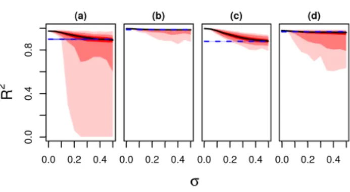
We first compare zero-sum regression and the LASSO with respect to the accuracy of predictions (Figure 1). Every plot shows the coefficient of determinationR²as a function ofσ, cf. supplementary material Fig.1 for the corresponding mean-squared errors (MSE). Hence, on the left we compare the performance of the LASSO and zero-sum regression for small changes of reference point, while on the right we compare it for large changes. Zero-sum regression is not affected by the change in reference point. Its performance is shown by the blue dashed horizontal lines. In contrast, LASSO is sensitive to the choice ofγi and yields different performances for each simulation run. The median of this distribution

0.0 0.2 0.4

0.00.40.8

(a)

0.0 0.2 0.4 (b)

0.0 0.2 0.4 (c)

0.0 0.2 0.4 (d)

R

2

σ

Fig. 1.Shown are the coefficients of determination,R²between observed and predicted responses, for the simulation studies (a) to (d) as a function ofσ, whereσis the standard deviation of the sample-specific shiftsγ_i. The median over all simulation runs is the blue dashed line for zero-sum regression and the solid black line for LASSO. The bright red, red and light red bands correspond to the LASSO and represent the 25 to 75%, 5 to 95% and 1 to 99% percentiles of theR²distribution obtained from drawing1000sets ofγ_i. The very narrow zero-sum bands are shown in blue.

is shown by the solid black lines while the 25 to 75%, 5 to 95% and 1 to 99% percentiles of the distribution are shown by bright red, red and light red bands, respectively. Depending on the correlation structure and the choice of theγizero-sum or the standard LASSO are more accurate. (a) In these simulations, the three relevant predictors,j= 1, . . . ,3, are highly correlated, the coefficientsβjdo not fulfill the zero-sum condition but vary in sign and size. For smallσ, zero-sum regression is inferior to the LASSO, but with increasingσzero-sum regression outcompetes the LASSO. We also observed several simulations where the classical LASSO breaks down completely yieldingR²values nearly zero. (b) This simulation is based on the same set of coefficients as scenario (a), but now the predictorx2

is anti-correlated tox1andx3. In spite of the change of reference point and the unbalanced coefficients both the LASSO and zero-sum regression work accurately. However, for largeσthe classical LASSO frequently looses predictive power and zero-sum regression is more reliable, even if the differences between the methods is much smaller than for scenario (a).

(c) Here, we have only positive coefficientsβj >0, which potentially spoils the zero-sum constraint. Note that the correlations are imposed as in scenario (a). Thus, we can directly study the consequences of changing the constantsβjto a scenario which more substantially violates the zero- sum condition. Interestingly, we qualitatively observe a similar trade-off between zero-sum bias and PRP-sensitivity as in the previous scenarios.

(d) Here, theβjadd-up to zero and no correlations are imposed on the predictor variables. Thus, for this scenario the zero-sum constraint is not a bias. Clearly, zero-sum works perfectly, while the LASSO breaks down rapidly in many of the simulations. In summary, zero-sum regression tends to outperform the LASSO forγithat are relatively large. More importantly, in several scenarios we observed a complete breakdown of the LASSO but never for zero-sum regression.

3.2 LASSO predictions change, if the reference point changes. Zero-sum predictions do not.

While it isa priorinot clear, whether a zero-sum or a LASSO model is more accurate, zero-sum models always have the advantage that predictions are reference point insensitive. In contrast, a LASSO model can be dominated by the reference point. To show the extend of PRP sensitivity of the LASSO, we compared predictions before and after changing the reference point (σ= 0versusσ ̸= 0), i.e., we compareyˆr₁toyˆr₂, while in the previous section we comparedyˆr₁toy. We used the same four simulation scenarios as in the previous section. Figure 2 summarizes the results. By definition, both predictions agreed for zero-sum regression, yielding a

(5)

0.0 0.2 0.4

0.01.02.03.0

(a)

0.0 0.2 0.4 (b)

0.0 0.2 0.4 (c)

0.0 0.2 0.4 (d)

MSE

σ

Fig. 2.Shown are the mean-squared errors (MSEs) calculated with respect to the predicted responses atσ= 0for the simulation studies (a) to (d) as a function ofσ, whereσis the standard deviation of the sample-specific shiftsγ_i. The median over all simulation runs is the blue dashed line for zero-sum regression and the solid black line for LASSO. The red and blue bands are analogous to Figure 1, but now represent the distribution of MSEs.

0.0 0.2 0.4

0.50.70.9

(a)

0.0 0.2 0.4 (b)

0.0 0.2 0.4 (c)

0.0 0.2 0.4 (d)

A UC

σ

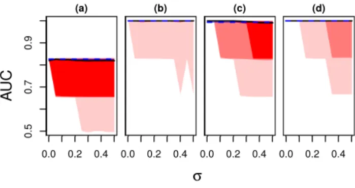
Fig. 3.Shown are the area under the ROC curves (AUCs) as a function ofσfor the simulation scenarios (a) to (d), whereσis the standard deviation of the sample-specific shiftsγ_i. The median over all simulation runs is the blue dashed line for zero-sum regression and the solid black line for LASSO. The red and blue bands are analogous to Figure 1, but now represent the distribution of AUCs.

mean-squared error of0, or perfect reproducibility. In contrast, for the LASSO we saw several simulations in all four scenarios where predictions vastly diverge upon changing the reference point.

3.3 Zero-sum regression facilitates reference point independent feature selection more reliably than the LASSO.

Besides prediction, feature selection is an important application of sparse regression models. If we use the LASSO, selected features depend on the reference point, if we use zero-sum they do not. In Figure 3 we show areas under the receiver operating characteristic (ROC) curve versusσ.

Again we used the scenarios (a) to (d) described above. In scenarios (b) to (d) zero-sum recovered the three driving features perfectly and so did the LASSO for the majority of simulations. However, in few simulations the LASSO picked incorrect features. In scenario (a) we never reached perfect feature selection. Nevertheless, zero-sum regression proved again to be more reliable. Note that an area under the curve (AUC) of0.5corresponds to random feature selection and in a few simulations the LASSO was not better than that. In summary, zero-sum regression selected relevant features as accurate as the LASSO. In few simulations the LASSO broke down due to change of reference point.

4 An application of zero-sum regression to genomic data integration: Identifying intestinal bacterial communities associated with indole production

In this section we show reference point insensitive data analysis at work. We chose a study that combined intestinal microbiome sequencing with metabolome analysis of urine in patients undergoing bone marrow transplantation. Different reference points apply to the intestine, the stool, and the urine of patients.

About 40% of patients receiving allogeneic stem cell transplants (ASCT) develop a systemic acute graft versus host disease (Ferraraet al., 2009). About 54% of these diseases affect the gastrointestinal tract (Martinet al., 1990). This complication was associated with the intestinal microbiome composition (Tauret al., 2012; Holleret al., 2014) and with the presence of toxic or the absence of protective microbiota born metabolites in the gut (Murphy and Nguyen, 2011). A candidate protective substance is the tryptophan microbial fermentation product indole (Weberet al., 2015).

It reduces epithelial attachment of pathogenic bacteria, promotes epithelial restitution and, simultaneously, inhibits inflammation (Bansalet al., 2010;

Zelanteet al., 2013).

Weber et al.(2015) studied associations between the microbiome composition of ASCT patients during treatment and urinary 3-indoxyl sulfate (3-IS) levels. 3-IS is a metabolite of indole produced in the colon and liver. In this study it was quantified in patient urine by liquid chromatography/tandem mass spectrometry. The intestinal microbiomes of the same patients were profiled by sequencing the hypervariable V3 region of the 16S ribosomal RNA gene in patient stool and mapping the sequences to operational taxonomic units (OTUs). ASCT patients receive antibiotics, which might kill indole producing bacteria thus damaging the intestine. If one identified the indole producing bacteria in the gut, one could choose antibiotics that spare them. As a first step towards this goal we strive to identify a small set of OTUs that are jointly associated with 3-IS levels.

This biomedical challenge defines a sparse high dimensional regression problem. And it is a regression problem where the choice of reference points matters. The reference point of the microbiome profiles is a fixed size aliquot of 16S rDNA obtained from bacteria in patient feces. The reference point that links the microbiome to 3-IS levels are patient intestines. If there are more indole secreting bacteria in the intestine, we expect more 3-IS in the urine. The total number of microbiota in patient intestines vary strongly due to diet and treatments including antibiosis. We thus expect that compositional microbiome data poorly reflects absolute microbiota abundances in the intestines. In summary, the regression problem calls for absolute bacterial abundances in patient intestines, while the available profiles provide only relative abundances. Obviously, the reference points do not match.

In total we analyzed 37 matched pairs of stool and urine specimens.

Urinary 3-IS was quantified by liquid chromatography tandem mass spectrometry (LC-MS/MS). To control for variations in urine flow rate, we normalized the measured concentration of 3-IS against the measured urinary concentration of creatinine (Waikaret al., 2010), which was also determined by LC-MS/MS. The intestinal microbiome was profiled by next-generation sequencing of the V3 hypervariable region of the 16S rRNA gene. Prior to DNA extraction of the stool samples, three exogenous bacteria (Salinibacter ruber, Rhizobium radiobacter, and Alicyclobacillus acidiphilus) were spiked into crude specimens as external controls. Subsequently, a constant aliquot of PCR amplified 16S rDNA was sequenced. Reads were assigned to160bacterial genera, one pseudo count was added, and the counts werelog₂transformed. Finally, the genera where quantified relative to two different reference points:

(6)

(i) We normalized the data sample-wise to a constant average of all genera.

This is equivalent to centering the data, cf. supplement.

(ii) We normalized the data to a constant average value of the 3 external standards.

Data (i) is library-size normalized (on log scale) and is thus the standard compositional microbiome. The reference point is a fixed size aliquot of 16S rDNA. This data does not reflect changes in the total microbial load of the stool. Data (ii), in contrast, is sensitive to changes in microbial load because in a fixed aliquot of 16S rDNA more endogenous sequences lead to proportionally less spike-in sequences. Here the reference point is a fixed size aliquot of stool.

We run the LASSO and zero-sum regression on both microbiome data sets withlog₂transformed urinary creatinine normalized 3-IS values as response variabley. 3-IS levels were predicted in leave one out cross validation and the predictions were compared to the measured values.

By definition zero-sum produces the same predictions for both datasets because of its PRP insensitivity.

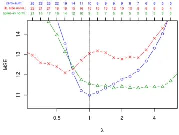
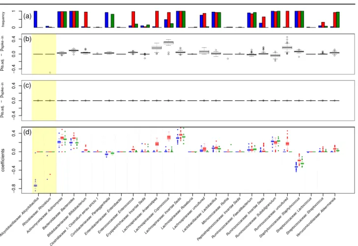
Figure 4 compares cross validated mean-squared errors of zero-sum regression (blue) with that of the LASSO for library-size normalized data (red) and spike-in calibrated data (green) as a function of the LASSO sparsity parameterλ. The optimal mean-squared errors are similar with zero-sum regression yielding the smallest error. More important in this application is the selection of features. Figure 5 summarizes our results, i.e. the selected features and the corresponding coefficients obtained in 37 models learned in a leave-one-out cross validation. Figure 5(a) shows how often a feature was selected. Features selected by the LASSO depended on the chosen reference point. For example,Bifidobacterium was frequently selected when the reference point was the library size but hardly ever, when the reference point was an external standard. Also when a feature was reproducibly selected for both reference points like the genus Staphylococcus, its regression coefficients can drastically differ depending on the reference point. Figure 5(b) shows the difference of regression weights for the two reference points. In theory, zero-sum regression should not be affected at all by the change in reference point. Indeed, this is observed in Figure 5(c). Finally, Figure 5(d) contrasts the regression coefficients of the LASSO with that of zero-sum regression. Interestingly unlike the LASSO, zero-sum regression picked the genus of one of the external standards,Alicyclobacillus, with a high negative weight. It thus automatically built its own reference point.

We tested if zero-sum regression retains its predictive power in the absence of external reference points. To this end we removed the three reference bacteria, Salinibacter ruber, Rhizobium radiobacter, andAlicyclobacillus acidiphilus, from the dataset and reperformed our analysis, cf. supplementary Figures 2 and 3. The lowest MSE observed in leave-one-out cross validation was10.86. This error is again lower for zero-sum regression than for the two LASSO models. In fact, it is even slightly lower than the error of the zero-sum regression with the spike-ins.

In summary, zero-sum regression stabilized feature selection compared to the LASSO. LASSO features greatly depended on the chosen reference point, zero-sum features did not. Zero-sum regression selects features that are predictive of urinary 3-IS independent of the reference point.

5 Discussion

Here we discussed the problem of reference point dependence in the analysis of omics data and exemplified its relevance both in a simulation study and in an application on integrating urinary metabolome data with intestinal microbiome compositions. We recommend zero-sum regression as a method that can overcome the problem. In this context, we contribute

11121314

λ

MSE

zero−sum:

lib. size norm.:

spike−in norm.:

26 23 23 22 19 14 11 10 8 9 9 9 8 7 6 6 5 5

22 21 21 18 16 15 16 15 15 13 12 10 10 8 8 8 5 4

21 18 17 16 14 12 10 9 8 7 6 6 5 5 5 3 3 3

0.5 1 2 4

Fig. 4.MSE in cross validation for different choices of the penalizing parameterλ. In blue zero-sum regression results (circles) and in red standard LASSO based on library-size adjusted data (crosses), and in green LASSO results based on spike-in normalized data (triangles). At the top of the figure the number of selected features is shown.

a coordinate descent algorithm for fitting zero-sum regression models and provide the first R-package for this type of analysis.

Our theoretical analysis is restricted to reference point changes that yield proportional data. On log-transformed data these proportional reference point changes are fully described by the sample specific shifts we discussed. Of course a reference point change can be more complicated leading to non-linear distortions. In this case zero-sum regression is no longer reference point independent. However, it might nevertheless be worth testing its performance, since it can still cushion the reference point, if the transformation systematically affects the sample mean.

We believe that there is a wide spectrum of high content profiling methods where changes or ambiguities of reference points exist and matter.

It ranges from gene and protein expression, via metabolomics, epigenetic readouts, microbiome sequencing, and metagenomics, to very recent advances in digital immune cell quantifications. More and more studies integrate several of these data types. Likely, the reference points differ between them. Also, the integration of new data with published data that can be downloaded from public repositories can greatly enhance analysis and interpretation. However, the reference points of the published data might not even be sufficiently clear from the documentation of the data files. We believe that in all these scenarios a reference point insensitive analysis is called for.

Finally, what does it mean, when we routinely say that a gene is up- regulated between control and treatment? These genes can be up-regulated with respect to one reference point but down-regulated with respect to another. A reference point insensitive analysis can not resolve this question, only meticulous distinction between reference points can. However, if we strive for more general statements like: "Gene A is up-regulated", we argue that these statements should at least be supported by a reference point independent analysis.

Acknowledgment

This work was funded by the German Cancer Aid (Grant 109548). We thank S. Mehrl and C.W. Kohler for carefully testing our software.

(7)

frequency 01

(a)

−0.40.00.4

βlib.adj.−βspike−in −0.40.00.4

βlib.adj.−βspike−in

●

● ● ●●●●

●

●●

●

●● ●

●

● ●

●

●●

●

●●

●

● ●

●

●● ●●

−0.8−0.40.00.4

coefficients

Alicyclobacillaceae: Alicyclobacillus Rhiz

obiaceae: Rhiz obium

Actinom ycetaceae: Actinom

yces

Bacteroidaceae: Bacteroides Bifidobacter

iaceae: Bifidobacter ium

Clostr idiaceae 1: Clostr

idium sensu str icto 1

Cor iobacter

iaceae: P araegger

thella

Enterobacter iaceae: Enterobacter

Enterococcaceae: Enterococcus Erysipelotr

ichaceae: Incer tae Sedis

Lachnospir aceae: Anaerostipes

Lachnospir aceae: Coprococcus

Lachnospir aceae: Incer

tae Sedis

Lachnospir aceae: Roseb

uria

Lachnospir aceae: uncultured

Lactobacillaceae: Lactobacillus Micrococcaceae: Rothia

Peptostreptococcaceae: Incer tae Sedis

Ruminococcaceae: F aecalibacter

ium

Ruminococcaceae: Incer tae Sedis

Ruminococcaceae: Subdoligr anulum

Ruminococcaceae: uncultured Staph

ylococcaceae: Staph ylococcus

Streptococcaceae: LactococcusStreptococcaceae: Streptococcus Verr

ucomicrobiaceae: Akk ermansia

Fig. 5.Comparison of zero-sum regression (blue) with LASSO applied to library-size (red) and spike-in (green) normalized data. In (a) it is shown how often a feature was selected (in

%). In (b) the differences of coefficients for the two LASSO models (library size versus spike-in) are shown. Fig. (c) shows the corresponding results for zero-sum regression. Figure (d) contrasts the regression coefficients of the LASSO models with that of zero-sum regression. All models are evaluated for the penalizing parameterλ= 1(for an analogous plot employing λ= 0.5see supplementary material).

References

Bansal, T., Alaniz, R. C., Wood, T. K., and Jayaraman, A. (2010). The bacterial signal indole increases epithelial-cell tight-junction resistance and attenuates indicators of inflammation.Proceedings of the national academy of sciences,107(1), 228–233.

Büttner, H. (1967). Bezugssysteme klinisch-chemischer analysen im gewebe und ihre aussagekraft. Zeitschrift für Klinische Chemie und Klinische Biochemie,5(5), 221–280.

Efron, B., Hastie, T., Johnstone, I., and Tibshirani, R. (2004). Least angle regression.The Annals of statistics,32(2), 407–499.

Ferrara, J. L., Levine, J. E., Reddy, P., and Holler, E. (2009). Graft-versus- host disease.The Lancet,373(9674), 1550–1561.

Friedman, J., Hastie, T., Höfling, H., Tibshirani, R.,et al.(2007). Pathwise coordinate optimization. The Annals of Applied Statistics,1(2), 302–

332.

Friedman, J. H., Hastie, T., and Tibshirani, R. (2010). Regularization paths for generalized linear models via coordinate descent. Journal of Statistical Software,33(1), 1–22.

Hastie, T., Tibshirani, R., and Friedman, J. (2009). The Elements of Statistical Learning: Data Mining, Inference, and Prediction, Second Edition. Springer Series in Statistics. Springer.

Hoerl, A. E. and Kennard, R. W. (1970). Ridge regression: Biased estimation for nonorthogonal problems.Technometrics,12(1), 55–67.

Holler, E., Butzhammer, P., Schmid, K., Hundsrucker, C., Koestler, J., Peter, K., Zhu, W., Sporrer, D., Hehlgans, T., Kreutz, M.,et al.(2014).

Metagenomic analysis of the stool microbiome in patients receiving allogeneic stem cell transplantation: loss of diversity is associated with use of systemic antibiotics and more pronounced in gastrointestinal graft- versus-host disease. Biology of Blood and Marrow Transplantation, 20(5), 640–645.

Krishnapuram, B., Carin, L., Figueiredo, M. A., and Hartemink, A. J.

(2005). Sparse multinomial logistic regression: Fast algorithms and generalization bounds.Pattern Analysis and Machine Intelligence, IEEE Transactions on,27(6), 957–968.

Lin, C. Y., Lovén, J., Rahl, P. B., Paranal, R. M., Burge, C. B., Bradner, J. E., Lee, T. I., and Young, R. A. (2012). Transcriptional amplification in tumor cells with elevated c-myc.Cell,151(1), 56–67.

Lin, W., Shi, P., Feng, R., and Li, H. (2014). Variable selection in regression with compositional covariates.Biometrika.

Martin, P. J., Schoch, G., Fisher, L., Byers, V., Anasetti, C., Appelbaum, F. R., Beatty, P. G., Doney, K., McDonald, G. B., and Sanders, J. E.

(1990). A retrospective analysis of therapy for acute graft-versus-host disease: initial treatment.Blood,76(8), 1464–1472.

Meier, L., Van De Geer, S., and Bühlmann, P. (2008). The group lasso for logistic regression.Journal of the Royal Statistical Society: Series B (Statistical Methodology),70(1), 53–71.

Murphy, S. and Nguyen, V. H. (2011). Role of gut microbiota in graft- versus-host disease.Leukemia & lymphoma,52(10), 1844–1856.

Nie, Z., Hu, G., Wei, G., Cui, K., Yamane, A., Resch, W., Wang, R., Green, D. R., Tessarollo, L., Casellas, R.,et al. (2012). c-myc is a universal amplifier of expressed genes in lymphocytes and embryonic

(8)

stem cells.Cell,151(1), 68–79.

Orlando, D. A., Chen, M. W., Brown, V. E., Solanki, S., Choi, Y. J., Olson, E. R., Fritz, C. C., Bradner, J. E., and Guenther, M. G. (2014).

Quantitative chip-seq normalization reveals global modulation of the epigenome.Cell reports,9(3), 1163–1170.

Taur, Y., Xavier, J. B., Lipuma, L., Ubeda, C., Goldberg, J., Gobourne, A., Lee, Y. J., Dubin, K. A., Socci, N. D., Viale, A., Perales, M.-A., Jenq, R. R., van den Brink, M. R. M., and Pamer, E. G. (2012). Intestinal domination and the risk of bacteremia in patients undergoing allogeneic hematopoietic stem cell transplantation. Clinical Infectious Diseases, 55(7), 905–914.

Tibshirani, R. (1996). Regression shrinkage and selection via the lasso.

Journal of the Royal Statistical Society. Series B (Methodological), 58(1), 267–288.

Waikar, S. S., Sabbisetti, V. S., and Bonventre, J. V. (2010). Normalization of urinary biomarkers to creatinine during changes in glomerular

filtration rate.Kidney international,78(5), 486–494.

Weber, D., Oefner, P. J., Hiergeist, A., Koestler, J., Gessner, A., Weber, M., Hahn, J., Wolff, D., Stämmler, F., Spang, R., Herr, W., Dettmer, K., and Holler, E. (2015). Low urinary indoxyl sulfate levels early after transplantation reflect a disrupted microbiome and are associated with poor outcome.Blood,126(14), 1723–1728.

Zelante, T., Iannitti, R. G., Cunha, C., De Luca, A., Giovannini, G., Pieraccini, G., Zecchi, R., D’Angelo, C., Massi-Benedetti, C., Fallarino, F., Carvalho, A., Puccetti, P., and Romani, L. (2013). Tryptophan catabolites from microbiota engage aryl hydrocarbon receptor and balance mucosal reactivity via interleukin-22. Immunity,39(2), 372–

385.

Zou, H. and Hastie, T. (2005). Regularization and variable selection via the elastic net.Journal of The Royal Statistical Society Series B-statistical Methodology,67(2), 301–320.