Abstract KatharinaSeelmann, * SteffenAßmann, ArneKörtzinger fi eldtests Characterizationofanovelautonomousanalyzerforseawatertotalalkalinity:Resultsfromlaboratoryand

Limnology and Oceanography.

doi: 10.1002/lom3.10329

Characterization of a novel autonomous analyzer for seawater total alkalinity: Results from laboratory and fi eld tests

Katharina Seelmann ,

* Steffen Aßmann,

Arne Körtzinger

1GEOMAR Helmholtz Centre for Ocean Research Kiel, Kiel, Germany

2Kongsberg Maritime Contros GmbH, Kiel, Germany

3Christian-Albrechts-Universität zu Kiel, Kiel, Germany

Abstract

High-quality seawater total alkalinity (A_T) measurements are essential for reliable ocean carbon and acidifica- tion observations. Well-established manual multipoint potentiometric titration methods already fulfill these requirements. The next step in the improvement of these observations is the increase of the spatial and tempo- ral measuring resolution with minimal personnel and instrumental effort. For this, a rapid, automated underway analyzer meeting the same high requirements as the traditional method is necessary. In this study, we carried out a comprehensive characterization of theflow-through analyzer CONTROS HydroFIA^®TA (Kongsberg Mari- time Contros GmbH, Kiel, Germany) for automated seawaterA_T measurements in the laboratory and infield with overall more than 5000 measurements. Under laboratory conditions, the analyzer featured a precision of1.5 μmol kg⁻¹and an accuracy of 1.0 μmol kg⁻¹, combined in an uncertainty of 1.6 –2.0 μmol kg⁻¹. High precision (1.1 μmol kg⁻¹) and accuracy (−0.32.8 μmol kg⁻¹), and low uncertainty (2.0 – 2.5μmol kg⁻¹) were also achieved duringfield trials of 4 and 6 weeks duration. Although a linear drift appears to be the typical behavior of the system, this can be corrected for by regular reference measurements giving con- sistent measurement results. Another advantage of regular reference measurements is the early detection of any kind of malfunction due to its direct impact on the measurement performance. Based on the present study, rec- ommendations for automated long-term deployments are provided in order to gain optimal performance char- acteristics, aiming at the requirements forA_Tmeasurements.

The total alkalinity (AT) of a seawater sample is defined by Dickson (1981) as “the number of moles of hydrogen ion equivalent to the excess of proton acceptors (bases formed from weak acids with a dissociation constant K≤10^−4.5 at 25C and zero ionic strength) over proton donors (acids with K> 10^−4.5) in 1 kg of sample.” Therefore, A_T is a measure of the seawater buffering capacity. Together with the other parameters, pH, pCO2, and total dissolved inorganic carbon (CT), it is one of the four measurable parameters that allow to analytically describe the marine carbonate chemistry using the corresponding thermodynamic relationships (Millero 2007). Therefore,AT measurements are essential components of ocean carbon observation. However, measuring this

parameter both precisely and accurately is very challenging due to its high background signal (A_T of average seawater≈2300μmol kg⁻¹) compared to the small natural var- iability in the open ocean (Millero et al. 1998; Lee et al. 2006) and the required high accuracy for reliable cross calculations.

The Guide to Best Practices for Ocean CO2 Measurements (Dickson et al. 2007) describes the most common standard method for measuring A_T based on a manual multipoint potentiometric titration of a seawater sample in an open or closed cell with a strong acid (here, hydrochloric acid). The method described there can achieve a precision (1σ) of better than 1 μmol kg⁻¹ and an overall bias of about 2 μmol kg⁻¹. This, however, requires exact weighing of the seawater sample within 0.01 g or a precisely calibrated, thermostatted pipette as a volume-based substitute. Furthermore, the calibration of the pH electrode used for the potentiometric titration must be carried out frequently to ensure proper pH measurements (Millero et al. 1993). Other disadvantages of the traditional method are the relatively long-measurement time per sample (approximately 10–20 min), the need of well-trained techni- cians in an air-conditioned laboratory, and the fact that the

*Correspondence: kseelmann@geomar.de

Additional Supporting Information may be found in the online version of this article.

This is an open access article under the terms of the Creative Commons Attribution License, which permits use, distribution and reproduction in any medium, provided the original work is properly cited.

measured seawater must be provided as a bottled and typically poisoned discrete sample. This procedure often expands the time period between the seawater sampling during afield cam- paign and the actual measurement in the laboratory. Further- more, a potential sampling error can significantly affect the quality of the AT measurement. Rapid seawater AT measure- ments at sea with a simple and robustflow-through analyzer that can also be operated in autonomous mode would over- come most of these challenges. Several authors described differ- ent automated flow-through measurement systems for seawaterA_Tusing potentiometric and spectrophotometric pH determination, respectively, with good accordance to the high- quality requirements (e.g., Roche and Millero 1998; Watanabe et al. 2004; Li et al. 2013). But none of these systems have become fully designed, commercially available products. At the time of this study, only the Submersible Autonomous Moored Instrument for alkalinity (SAMI-alk) that was developed and tested by Spaulding et al. (2014) was available as a product for unattended A_T measurements. Its measurement principle is based on a tracer monitored titration approach, introduced by Martz et al. (2006) using a colorimetric tracer for simultaneous pH detection and acid concentration determination.

In this study, we test the CONTROS HydroFIA^®TA, a novel commercially available flow-through analyzer for autonomous seawaterATmeasurements built by Kongsberg Maritime Contros GmbH. Its general principle is based on open-cell single-point titration with spectrophotometric pH determination. Here, we report the results of a suite of experiments carried out with this novel instrument both in the laboratory and in thefield, that is, two major research cruises to the North and South Atlantic Ocean. The goal of this study is to characterize the performance of the analyzer as well as its behavior under laboratory and real field conditions in view of potential long-term deployments. In order to evaluate, whether the measurement quality of the ana- lyzer is suitable for underway AT measurements in the open ocean, we compare the results with quality targets stated within the oceanographic community’s established guides: (1) The

“Guide to best practices for ocean CO2 measurements” by Dickson et al. (2007) provides precision (standard deviation,σ) and accuracy (bias,ΔAT) requirements for standard open-cellAT

titrators. (2) The “Global Ocean Acidification Observing Net- work: Requirements and Governance Plan” by Newton et al.

(2015) provides uncertainty targets forATmeasurements in order to identify relative spatial patterns and short-term variations (“weather”goal), and to assess long-term trends with a defined level of confidence (“climate” goal), respectively. These targets

are particularly important for the ocean acidification observing community. It must be taken into account that the requirement for the“climate”goal is“only achievable by a very limited num- ber of laboratories and is not typically achievable for all parame- ters by even the best autonomous sensors”(Newton et al. 2015).

The certain targets of both guidelines are outlined in Table 1.

Materials and methods

Measurement principle

The measurement principle of the analyzer is oriented to the open-cell titration as described in the Guide to Best Practices for Ocean CO₂Measurements (Dickson et al. 2007). Accordingly, a known amount of seawater is titrated with a solution of hydrochloric acid (HCl) to afinal pH of about 3.0–3.5. A mixing and degassing procedure allows the escape of all CO₂deliber- ated from the sample’s dissolved inorganic carbon content. The guide describes a potentiometric pH monitoring of the mixture over the entire titration. Following the definition of total alka- linity (Dickson et al. 2007),A_Tat any titration point is given by

−msw×AT+mA×CA

msw+mA = H½ ⁺F+ HF½ + HSO ⁻₄

+ H½ 3PO4−HCO₃⁻

−2×CO²⁻₃

−B OHð Þ₄⁻

−½OH⁻−HPO²⁻₄

−2×PO³⁻₄

−SiO OHð Þ₃⁻

−½NH3−½HS⁻ ð1Þ

where [H⁺]Fis the free concentration of hydrogen ions,mswis the mass of the seawater sample, and mA is the mass of the added acid with the concentrationCA. Due to the working pH range of 3.0–3.5 and complete CO2removal, the majority of the terms in Eq. 1 can be ignored (Dickson et al. 2003). Hence, Eq. 1 can be reduced to

−msw×AT+mA×CA

msw+mA

= H½ ⁺F+ HF½ + HSO ₄⁻

ð2Þ

Deviating from the guide, the used analyzer determines the pH spectrophotometrically through a single-point titration of the seawater similar to theATmeasurement principle of Yao and Byrne (1998) and Li et al. (2013). Here, the titrant consists of two separate solutions: An acid (HCl) and an indicator solu- tion of bromocresol green sodium salt (BCG). Based on the definition of Dickson (1981), the added BCG is regarded as a proton donor in the sample-titrant mixture due to its dissocia- tion constant KI at 25C being slightly greater than 10^−4.5 (exact definition ofKI later in this section, seeEq. 11). Thus, Eq. 2 must be extended by an indicator term

−msw×AT+mt×Ct

msw+mt

= H½ ⁺F+ HF½ + HSO ₄⁻

+ HI½ ⁻ ð3Þ

where [HI⁻] is the concentration of the protonated (i.e., acidic) form of BCG, mt is the sum of the masses of the two titrant Table 1.Quality targets.

Dickson et al. (2007) Newton et al. (2015)* Precision (1σ):1μmol kg⁻¹ “Weather”goal:u(c) = 10μmol kg⁻¹ Accuracy (ΔAT):2μmol kg⁻¹ “Climate”goal:u(c) = 2μmol kg⁻¹

*Uncertainties with 68.3% confidence interval.

solutions (mt=macid+mindicator), andCtis the acid concentra- tion in the combined titrant solution. Here, it is calculated by:

Ct=CA×mA

mt ð4Þ

For a spectrophotometric pH detection using BCG as indi- cator, the ideal pH range of the sample-titrant mixture is around an absorbance ratio (R) of R≈1 (further explanation later in this section). This corresponds to a pH range of about 3.5–4.0 and is achieved by adjusting the amount of added acid. Li et al. (2013) show that the reduction of Eq. 1 to Eq. 2 is also valid for this pH range, provided that CO₂is quantita- tively removed. Furthermore, within an autonomous measure- ment routine, volumes are easier to handle than masses.

Hence, Eq. 3 is modified to

−Vsw×ρsw×AT+Vt×ρt×Ct

Vsw×ρsw+Vt×ρt

= H½ ⁺F+ HF½ + HSO ₄⁻

+ HI½ ⁻ ð5Þ

whereVswandVtare the volumes of the seawater sample and the added titrant, respectively, andρswandρtare the densities of the seawater sample and the added titrant, respectively. Fol- lowing Li et al. (2013), a volume mixing ratioγv(γv=Vsw/Vt), a density ratio γρ (γρ = ρsw/ρt), and a mass mixing ratio γ (γ=γv×γρ) are introduced to simplify the equation:

−γ×AT+Ct

1 +γ = H½ ⁺F+ HF½ + HSO ₄⁻

+ HI½ ⁻ ð6Þ

The last three terms in Eq. 6 can be calculated using the dis- sociation equilibria described in Dickson et al. (2007). An addi- tional rearrangement leads to

AT×γ=Ct−ð1 +γÞ

× ½H⁺F+ST×_{1 +}^γ_γ×½H⁺F

H⁺

½ F+KS

+FT×_{1 +}^γ_γ×½H⁺F

H⁺

½ F+KF

+IT×_{1 +}¹_γ×½H⁺F

H⁺

½ F+KI

!

ð7Þ

whereS_TandF_Tare the total sulfate and the totalfluoride con- centration in the seawater sample,I_Tis the total BCG concen- tration in the titrant,KSandKFare the dissociation constants of HF and HSO₄⁻ andKIis the second dissociation constant of BCG. The factors γ/(1 +γ) and 1/(1 +γ) represent the dilution factors of the seawater sample and the titrant, respectively.

In Eq. 7, all dissociation constants are on the free scale, and concentrations are given in moles per kilogram solution (mol kg⁻¹). The free concentration of hydrogen ions, [H⁺]F, or pHF, in the sample-titrant mixture is measured spectrophoto- metrically. Following Breland and Byrne (1993) and Yao and Byrne (1998), pH_Fis described by

pH_F=−logKI+ log R−e1

e2−R×e3

ð8Þ

with

e1=λ2εHI⁻

λ1εHI⁻

e2=λ2εI²⁻

λ1εHI⁻

e3=λ1εI²⁻

λ1εHI⁻ ð9Þ and

R=A_λ2

A_λ1 ð10Þ

wheree1,e2, ande3represent ratios of absorption coefficients, λiεxfor each indicator form,x, at wavelength 1 (λ1) and 2 (λ2), where the acid (HI⁻) and the base indicator form (I²⁻) have their absorbance maxima.R is the absorbance ratio atλ1and λ2. For BCG, the following values are available from the litera- ture:λ1= 444 nm,λ2= 616 nm,e₁= 0.0013,e₂= 2.3148, and e₃= 0.1299;e₁,e₂, ande₃are considered to be independent of salinity (Breland and Byrne 1993; Yao and Byrne 1998).

Breland and Byrne (1993) reported the salinity dependence (20≤S≤35) ofK_Ifor BCG at 25C as

−logKI= 4:4166 + 0:0005946×ð35−SÞ ð11Þ

whereS is the salinity of the seawater sample. Yao and Byrne (1998) described an advanced salinity range up to 37 for this dependence. Due to the dilution of the seawater sample by the reagents made up in deionized (DI) water, the salinitySof the sample-titrant mixture must be adjusted as follows:

isw= 0:72× S

35 ð12Þ

imix=isw×Vsw×ρsw+CA×VA×ρA+CBCG×VBCG×ρBCG

Vsw×ρsw+Vt×ρt ð13Þ Smix= 35× imix

0:72

ð14Þ

whereiswandimixare the ionic strengths of the seawater and the seawater-titrant mixture, respectively,V_BCGandρBCGare the vol- ume and the density of the added indicator solution with the BCG concentrationC_BCG,V_AandρAare the volume and the den- sity of the added HCl solution, andSmixis the resulting salinity of the seawater-titrant mixture. This calculation assumes the activ- ity coefficient of BCG to be 1 and that a salinity of 35 corresponds to an ionic strength of 0.72 (Dickson 1990). Hence, the pH of the seawater-titrant mixture at 25C within the valid salinity range of 20–37 can be calculated as follows:

pH_F= 4:4166 + 0:0005946×ð35−SmixÞ+ log R−0:0013 2:3148−R×0:1299

ð15Þ

For this calculation, Breland and Byrne (1993) also described the temperature effect on the absorbance measure- ments between 18C and 32C as follows:

R25=Rt×½1 + 0:00907×ð25−tÞ ð16Þ

whereR25andRtare the absorbance ratios at 25C and at the exact temperature t (C) of the sample-titrant mixture, respectively.

Finally, theATof a temperature controlled seawater sample with known salinity can be determined by a spectrophotomet- ric pH measurement using Eqs. 7, 15, and 16. Almost all vari- ables in these equations are known or can be calculated. For the present analyzers, the volumes of the added reagents (Vt=VHCl+VBCG) arefixed and thus known due to the usage of injections loops with a defined length of tubing (see

“Instrumental design” section). The densities (ρsw and ρt) at the measured temperatures of the seawater sample with known salinity, and the reagents with known chemical com- position were determined using the equations reported in Dickson et al. (2007). The calculation of KS and KF is also based on the equations of Dickson et al. (2007) using the salinity of the seawater-titrant mixture; the calculation basis ofSTandFTis their well-characterized relationship to seawater salinity.

Due to the character of an absolute method, a calibration is principally not necessary. However, the exact volume of the seawater sample Vsw is the only unknown variable, which must be practically determined utilizing a one point certified reference material (CRM) measurement. With the knownAT

value of the CRM, it is possible to calculateVswusing the same equations as forATdetermination. Consequently, all inevita- ble uncertainties (e.g., errors in the dissociation constants, the exact concentration of the titrant, impurities of the indicator dye or minor uncertainties in the titrant volume) are com- bined inVsw and thereby taken into account for subsequent ATmeasurements.

Instrumental design Analyzer setup

For this study, we used two units of the commercially avail- able AT analyzer CONTROS HydroFIA^® TA (Kongsberg Mari- time Contros GmbH, Kiel, Germany). For simplification, they are called“red system”and“gray system”in the following sec- tions due to their different housing color. Otherwise, as long as there is no other information provided, the two analyzers can be regarded as being identical. Figure 1 shows the sche- matic setup of the analyzer showing the involved components in the measurement routine.

The acid and indicator reservoirs are closed and kept in gas- tight and light-tight bags preventing any alteration of the solutions. Both solutions are separately pumped by piston pumps through injections loops with fixed length and thus fixed volume. These loops are used for injection into the sam- ple circuit using injection valves. The injection valves are con- nected to the sample circuit in which the solution is pumped by a membrane pump. Depending on the position of the tan- dem valve, the sample solution is circulated within the sample

circuit or is pumped through the open circuit to waste. While circulating, the sample is constantly temperature controlled to 25C by the heat exchanger and at the same time the CO2is removed by the degassing unit, which is combined with the heat exchanger (seeFig. 2). The temperature control is realized by a Peltier element and temperature measurement directly behind the cuvette. CO2removal is done by soda lime behind a membrane. The absorption measurement for the pH detec- tion is realized by means of aflow-through cuvette with 1 cm path length, a broad-band white LED light source and a CCD spectrometer resolving the full absorption spectrum. With this setup, both can be measured simultaneously, the two Fig. 1.Schematic diagram of the CONTROS HydroFIA^®TA system setup.

Solid lines representfluid paths for sample water, acid, or indicator solu- tion. Dashed lines are light paths for the absorption measurement. Dotted lines are for naming and description. Oval forms represent reservoirs for the respective solutions. The indicator and acid reservoirs are closed while the feed and waste reservoirs are open.

Fig. 2.Schematic diagram of the degassing/heat exchange unit. The sam- ple solution isflowing through theflow path being connected to tubing leading to the other parts of the measurement system (compare Fig. 1).

For temperature control of the sample solution, the titanium heat exchange area is used separating the Peltier element from thefluid. For CO2strip- ping, the membrane gas exchange area is used separating the soda lime from thefluid.

absorption maximums of the indicator dye (444 and 616 nm) for pH calculation as well as the nonabsorbing wavelength 730 nm for correction of a potential baseline shift during the measurement routine.

Differences between used systems

For evaluating different working ranges of the analyzers during the secondfield study (see“Experiments”section), each analyzer was equipped with different lengths of acid loop tub- ing. The red system was equipped with tubing 14.5% longer than the gray system resulting in a lowerfinal pH value after acid addition when measuring at a givenAT. Due to further developments of the analyzer during the course of this study, the red and the gray system were equipped with a modified degasser unit leading into a longer degassing time. The change was done after thefirstfield deployment.

Measurement routine

TheAT measurement routine for each sample is structured as follows: (1) The sample pumpflushes all tubing with fresh seawater to remove the residual solution from the previous analysis run. (2) This is followed by a conditioning phase with stopped seawaterflow, where the system is conditioned to the pH of seawater to avoid memory effects from the large pH changes during the measurement. (3) Another flush routine collects the seawater sample for the actual measurement (either from a continuous seawaterflow or a connected sample bottle), followed by the closing of the sample loop. (4) Now, the sample treatment starts. Dark and blank spectra are mea- sured with the untitrated sample in the cuvette. (5) Both injec- tion loops are filled with HCl solution and BCG solution, respectively, and the reagents are simultaneously injected into the sample loop. (6) This sample-titrant mixture is continu- ously pumped in the closed loop until completely homoge- nized. During this, the degasser unit, which is included in the sample loop, removes the CO2across a membrane, while con- stantly controlling the sample temperature to 25.00.1C.

(7) After equilibration and degassing, which takes about 5 min, the spectra of the CO2free and fully temperature con- trolled sample-titrant mixture are measured in the cuvette, and theATof the seawater sample is calculated following the equations in “Measurement principle” section. The whole measurement cycle (maximum measurement frequency) took approximately 7 min during the first field experiment and approximately 10 min with the modified degasser membrane during the secondfield test.

Seawater sample treatment

Bottled samples (i.e., CRM) were connected to the analyzer with PVC tubing using the same inlet as for underway measure- ments without any pretreatment. For autonomous underway measurements, the system was installed in bypass to a continu- ously pumped seawaterflow using PVC tubing. Due to the very small tubing diameters of 0.8 mm inner diameters inside the system, the seawater was filtered using a flow-through filter

with 50μm pore size on the first cruise and a cross-flowfilter with 0.2μm pore size on the second cruise. Thesefilters only remove particular matter (e.g., sediment particles) which is important for not having particles dissolved during the sample treatment routine of the analyzer thus altering theATmeasure- ment result. An adsorption of dissolved organic matter (DOM) onto thefilter material interfering withATmeasurement is not given to our knowledge. Furthermore, within the scope of this study, DOM contributions toATare not significant in the open ocean (e.g., McElligott et al. 1998; Lee et al. 2000; Millero et al.

2002, Ko et al. 2016).

Solutions and standards

The concentration of the used HCl and BCG solution was 0.1 mol kg⁻¹and 0.002 mol kg⁻¹, respectively. Both reagents were made up in DI water and provided custom-made and in ready-to-use cartridges by Kongsberg Maritime Contros GmbH. The BCG solution was made up by dissolving the sodium salt of BCG. The used BCG was not purified, but the development of a high perfromance liquid chromatography (HPLC) purification method for BCG and testing its impact on theA_Tmeasurement is in progress and will be described else- where. CRM (batches 142, 143, 150, and 160) was obtained from A. G. Dickson at the Scripps Institution of Oceanography of the University of California, San Diego. For laboratory experiments, a seawater substandard was prepared out of left- over seawater samples poisoned with mercury chloride. For this, the samples were freshly mixed and the resultingA_Twas measured using the reference method (see below).

Reference measurements

For accuracy monitoring, the analyzer measured CRM daily throughout all field campaigns. Every morning and evening, five repetitive CRM measurements were carried out. Further- more, the measurements of the analyzer were compared to the results from discrete seawater samples measured on a standard open-cell alkalinity system using potentiometric titration (VINDTA 3S, Marianda, Germany). For these mea- surements, discrete samples were on average taken twice per day throughout all field campaigns and measured in the home lab (GEOMAR Helmholtz Centre for Ocean Research Kiel, Germany) following the recommendations in Dickson et al. (2007).

Statistical calculations

For evaluating the precision of the system both in the labo- ratory and in field, the standard deviation σ of consecutive measurements of a reference sample (e.g., CRM) is calculated as follows:

σ=

ffiffiffiffiffiffiffiffiffiffiffiffiffiffiffiffiffiffiffiffiffiffiffiffiffiffiffiffi Pn

i= 1ðxi−xÞ² n−1 s

ð17Þ with

x=1

n×Xⁿ

i = 1

xi ð18Þ

wherenis the number of measurements,x_iis thei^thmeasure- ment of n measurements, and x is the mean of the measurements.

For evaluating the accuracy in field, the biasΔA_T between theA_T value of the system and the A_Tvalue of the reference sample (CRM and discrete samples) is calculated as follows:

ΔAT=AT,Analyzer−AT,Reference ð19Þ

The accuracy in the laboratory is determined in a different way and will be explained in the “Results and discussion” section.

In order to compare the measurement quality of the ana- lyzer with the targets of the ocean acidification observing community (Newton et al. 2015), an approximation of the standard uncertainty both in the laboratory and infield is nec- essary. Due to the usage of CRM for“calibration”and valida- tion of the analyzer, we utilize the within-laboratory validation approach of measurement uncertainty estimation known as“top down”for thefirst approximation of the mea- surement uncertainty. The best-known formalization of this approach is the so-called Nordtest™described by Magnusson et al. (2017), which is based on the guide by Ellison and Wil- liams (2012). Therefore, the combined standard uncertainty u(c) (approximates to a 68.3% confidence interval) is calcu- lated by:

uð Þc =

ffiffiffiffiffiffiffiffiffiffiffiffiffiffiffiffiffiffiffiffiffiffiffiffiffiffiffiffiffiffiffiffiffiffiffiffiffi uðRwÞ²+uðbiasÞ²

q ð20Þ

whereu(Rw) is the uncertainty estimate of the precision (ran- dom effects) andu(bias) is the uncertainty estimate of possible laboratory and procedural bias (systematic effects).

Experiments

Laboratory experiments Scope

The first part of this study consists of experiments carried out under laboratory conditions. This means that the analyzer did not run for longer than 200 consecutive measurements (equaling approximately up to 24 h) and was set up in an air- conditioned room. Furthermore, the system was shut off over- night between the measurement days. At the start of each measurement day, the analyzer carried out several condition- ing measurements to ensure good system stability.

Performance characteristics

Tests on the performance characteristics in the laboratory were carried out as standard addition experiment. Therefore, a stable seawater sample (relatively highAT) was titrated with a HCl solution (0.1 mol kg⁻¹) to lower its AT in five steps

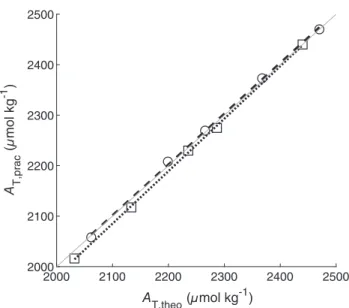
(general range of resulting AT: 2000–2450μmol kg⁻¹). The titration was carried out by adding different precisely known volumes of HCl to a known volume of seawater resulting in five seawater aliquots with stepwise decreasingAT. The theo- reticalAT (AT,theo) was calculated from the volumes of added acid and seawater, the concentration of the acid, and the origi- nalATof the seawater. To determine the practicalAT(AT,prac), each of these aliquots was repeatedly measured with the ana- lyzer forfive times. This experiment was carried out for each analyzer before and after the cruises.

Overlapping Allan experiment

Regular reference measurements are obligatory for quality assurance and performance monitoring of the analyzer during long-term deployments. To achieve best results, the optimal number of repeated reference measurements with the smallest averaging error had to be determined. For this, we performed a stability estimation by determining the overlapping Allan deviation at different averaging times. To improve the confi- dence of the stability estimate, we used the overlapping Allan deviation instead of the normal Allan deviation. The over- lapping Allan deviation σy(τ) makes maximum use of the data set by utilizing all possible combinations of samples at each averaging time τ (Riley 2008). It is estimated by the expression

σyð Þτ =

ffiffiffiffiffiffiffiffiffiffiffiffiffiffiffiffiffiffiffiffiffiffiffiffiffiffiffiffiffiffiffiffiffiffiffiffiffiffiffiffiffiffiffiffiffiffiffiffiffiffiffiffiffiffiffiffiffiffiffiffiffiffiffiffiffiffiffiffiffiffiffiffiffiffiffiffiffiffiffiffiffiffiffiffiffiffiffiffiffiffiffiffiffiffiffiffiffiffiffiffiffiffiffiffiffiffiffiffiffiffiffiffiffiffiffiffiffiffiffiffi 1

2×AF²×ðn−2×AF + 1Þ×ⁿ⁻²X^{×AF + 1}

j= 1

X

j+ AF−1 i=j

y_{i+ AF}−y_i

½

8<

:

9=

; v 2

uu ut

ð21Þ

wherenis the total number of measured samples,τis the aver- aging time that is calculated asτ = AF ×τ0, where AF is the averaging factor andτ0is the basic measurement interval, and y_iis thei^thofnfractional frequency values averaged overτ. In this experiment,nwas the total number ofATmeasurements (n = 30), τ0 was the measurement interval of the analyzer (τ0= 10 min), AF was the number of averaged replicates of the reference measurement, andyrepresented theATvalues. In an optimal system with only statistical noise, a higher number of averaged replicates, that means longer averaging time, would lead to a higher precision of the measurement. How- ever, due to long-term drift effects on the analyzer, the Allan deviation starts to increase again at some point. The minima in the overlapping Allan plot (σy(τ) vs. AF) indicate the opti- mal number of averaged replicates. For this experiment, a sta- ble seawater substandard was repeatedly measured 30 times in row with a measurement interval of 10 min on four different measurement days.

Field experiments Scope

In order to test the performance of the analyzer underfield conditions, we participated in two major research cruises: RV

Meteor cruise 133(M 133), from Cape Town, South Africa to Port Stanley, Falkland Islands; 15 December 2016–13 January 2017, and RV Maria S. Merian cruise 68/2 (MSM 68/2), from Emden, Germany to Mindelo, Cape Verde; 03 November 2017–14 November 2017. In both cases, the analyzer mea- sured continuously pumped surface seawater (underway mea- surement mode) during the entire cruise with the fastest measurement interval of 7 min during M 133 and 10 min dur- ing MSM 68/2, except when separate experiments were carried out. The different intervals were due to the degasser mem- brane change as mentioned in“Instrumental design”section.

While we only used the red system on cruise M 133, we had the possibility to run both the red and gray system in par- allel on cruise MSM 68/2.

At the beginning of both cruises, each analyzer performed several conditioning measurements to ensure system stability.

After stabilization, the internal seawater sample volume was determined with a freshly opened CRM.

Working range

Due to the measurement principle of the system, the work- ing range of the analyzer is limited by the pKa value of BCG, its absorption coefficients of the acid and base form and the absorbance ratioRof the sample-titrant mixture, and therefore by the resulting pH of the sample-titrant mixture. The final pH value of a sample with givenATafter acidification can be freely adjusted by the amount of added acid or its concentra- tion to meet the range of seawater AT in the measured area.

The AT range is limited to seawater with salinities between 20 and 37 as specified by the characterization of BCG (Breland and Byrne 1993; Yao and Byrne 1998). Due to the constant temperature control of the sample water to 25C, there is only the limitation of the analyzer’s temperature controlling capa- bility ranging from 5C to 30C for in situ temperatures. To take advantage of two analyzers running in parallel during the MSM 68/2 cruise, the influence of two different acid volumes was tested. For this, each analyzer was equipped with different lengths of acid loop tubing (see “Instrumental design” sec- tion). The goal of this experiment was to investigate the influ- ence of different pH ranges on the performance of the measurements. This experiment was only carried out on cruise MSM 68/2.

Performance characteristics

The precision underfield conditions was evaluated by mea- suring CRM on both cruises. Additionally, during the cruise M 133, a long-term precision experiment was conducted. For this, a stable seawater substandard was prepared and measured 178 times consecutively with a measurement interval of 7 min.

The accuracy evaluation was carried out by comparing the measurements of the analyzer with both the certified values of the CRM (twice per day throughout both cruises), and theAT

values of taken discrete samples (on average twice per day throughout both cruises) measured with the reference system VINDTA 3S.

Initial drift after idle time

For longer idle times (≥1 d), it is recommended toflush the analyzer with DI water to avoid any deposits inside the tubing, for example, from the last colored and acidified sample. These idle times could be necessary, for example, during harbor time between field campaigns. Harbor seawater often is very dirty and should not be run through the system. Since the analyzer is flushed with DI water, the system is conditioned to low ionic strength, causing an extended stabilization phase (initial drift) when measuring again after these idle times. To examine the extent of such a drift, the system was flushed with DI water and did not measure any sample for 48 h, except for the veryfirst measurements at the beginning of the cruise. There- fore, the initial idle time matched the storage and transporta- tion time of the analyzer before the cruise (≈3 months).

Afterward, a seawater substandard taken during the cruise was measured until the measurements were stable (standard devia- tion of the last three measurements≤2μmol kg⁻¹). This 48-h idling experiment was carried out three times during the whole cruise M 133: at the beginning, after 1304 measure- ments, and after 2183 measurements.

Results and discussion

Laboratory experiments Performance characteristics

The comparison and discussion of the laboratory perfor- mance before and after afield deployment is most useful for an analyzer without any hardware problems during this deployment. Consequently, only the results for the red system before and after the MSM 68/2 cruise are shown and inter- preted in the following part as the gray system suffered from a leakage in the degasser unit (see “General information” section later in this study). Figure 3 shows the results of the standard addition experiment observed with the red system before and after the MSM 68/2 cruise. For accuracy evaluation in the laboratory, the root mean square error (RMSE) of the measuredATvalues was determined as follows:

RMSE =

ffiffiffiffiffiffiffiffiffiffiffiffiffiffiffiffiffiffiffiffiffiffiffiffiffiffiffiffiffiffiffiffiffiffiffiffiffiffiffiffiffiffiffiffiffiffiffiffiffiffiffiffiffiffiffiffiffiffiffiffiffi 1

n×Xⁿ

i= 1

AT,fitted,i−AT,prac,i

2

vu

ut ð22Þ

wherenis the number of titration steps,A_T,fitted,iis thei^thATvalue calculated with the linear regression equation withAT,theo,i as xvariable. Before the campaign, the RMSE was determined with 5.5μmol kg⁻¹; afterward, it is improved to1.0 μmol kg⁻¹. This big difference is due to a change of the experiment proce- dure. Before the cruise, the titrated seawater samples were manu- ally changed and each measurement was started by hand.

Afterward, a more optimized experiment procedure was applied using an autosampler for these purposes. This custom-made auto- sampler is part of the system calibration setup at the Kongsberg Maritime Contros GmbH laboratory and is used for routine cali- brations automatically changing sample solutions of definedAT

levels. By using this autosampler, uncertainties, caused by the operator, are partly removed resulting in better performance of the experiment itself. Furthermore, due to the worse slope and the large intercept of the linear regression of the data set before the cruise, it is possible that some unknown additional errors occurred during the experiment. However, the after-cruise evalu- ation shows a very satisfactory correlation betweenA_T,pracand A_T,theo with a slope of 1.010.02 and an intercept of

−11.440.6 which are as expected (slope = 1, intercept = 0) within their found uncertainty. Furthermore, its laboratory accu- racy of1.0 μmol kg⁻¹is in full agreement with the require- ments of Dickson et al. (2007) for the standard A_T titration methods for which an accuracy of2μmol kg⁻¹is required.

The precision in the laboratory is determined by using the standard deviation of thefive single measurements at each titra- tion step. General precision for each titration step was found to be approximately 2 μmol kg⁻¹ for this analyzer (data not shown). This general precision also agrees with precision values determined by Kongsberg Maritime Contros GmbH for any HydroFIA analyzer. The explained laboratory performance char- acteristic is a standard procedure at Kongsberg Maritime Contros GmbH for each CONTROS HydroFIA^®TA system and is carried out regularly. A performance characteristic test carried out with the gray system after the MSM 68/2 cruise and maintenance of the manufacturer (no leakage) shows an overall precision of 1.5μmol kg⁻¹. Because both analyzers are treated similarly in the laboratory, and the modified method with autosampler is

stable, robust and part of the quality management system of the company, it is possible to generalize this precision for all labora- tory performance characteristics.

For estimating the combined standard uncertainty of this experiment in the laboratory (only shown for after-cruise experi- ment), the laboratory precision was utilized as random uncer- tainty component and the RMSE of the measuredATvalues as systematic uncertainty component, respectively. Both compo- nents were estimated with a freshly“calibrated”analyzer using CRM. The relative combined laboratory standard uncertainty was estimated at 0.08%, which results in a combined laboratory standard uncertainty of 1.6–2.0μmol kg⁻¹atATvalues from 2000 to 2450μmol kg⁻¹(seeSupporting Information for more details of the calculations). This laboratory uncertainty approximation is in full agreement with the “weather” goal requirements of Newton et al. (2015). Even the very high requirement of the“cli- mate”goal is achieved. Thus, the laboratory standard uncertainty of the analyzer is sufficient for ocean acidification measurements.

Overlapping Allan experiment

Figure 4 shows the results of the overlapping Allan analysis with each curve representing one specific measurement day. As expected, each Allan plot shows a minimum representing the optimal number of averaging replicate measurements. The minima range fromA = 3–6 with resulting overlapping Allan deviations σy(τ) of 0.5–1.0 μmol kg⁻¹, each determined at A_T≈2270μmol kg⁻¹ (pHsample-titrant mixture≈3.6). This means that a reference sample used for performance monitoring should be repeatedly measured at least three times to minimize the impact of statistical noise. On the other hand, more than six

2000 2100 2200 2300 2400 2500

A_T,theo (µmol kg^-1) 2000

2100 2200 2300 2400 2500

A T,prac (µmol kg-1 )

Fig. 3._AT,pracas a function ofAT,theoof each titration step measured with the red system before (open squares) and after (open circles) the MSM 68/2 cruise in the laboratory.AT,pracis the average offive repeated measurements for each aliquot. The black dashed and dotted line indi- cates the linearfit of the data points with the following resulting linear equations: Before:y= (1.030.01)×x−(97.628.4),R²= 0.999, and after:y = (1.010.02)×x−(11.440.6), R² = 0.999. The gray solid line indicates the 1-to-1 line of this plot.

0 1 2 3 4 5 6 7 8 9 10 11 12 13 AF

0 0.2 0.4 0.6 0.8 1 1.2 1.4 1.6 1.8

y() (µmol kg-1 )

Fig. 4.Overlapping Allan deviationsσy(τ) as a function of the number of averaged replicates of the reference measurement, AF. Each curve repre- sents one measurement day. The gray area indicates the range of the observed minima in the experiments.

repetitions lead into a regime affected by instrument drift or changes of environment/sample solution and causes the preci- sion to deteriorate. The ideal number of repeated reference mea- surements depends on different factors: The available volume of stable reference seawater during the deployment, the length of the deployment, and the required number of quality assurance measurements per day. In addition, possible outliers within these reference measurements should be taken into account. For the performance monitoring during the two research cruises, we decided to repeatedly measure the reference samples (here, CRM) five times every morning and evening.

Field experiments General information

During the MSM 68/2 cruise, the red analyzer ran without any hardware problems. Consequently, its performance char- acterization is discussed in detail in the following parts. How- ever, because of the early development level of the system, both the M 133 analyzer as well as the gray analyzer during the MSM 68/2 cruise suffered from a leakage in the degasser unit. The effects of such a malfunction on the performance are briefly discussed afterward.

Underway measurements

To give an overview of the measured underway variables (A_T, sea surface salinity [SSS] and sea surface temperature [SST]) in the monitored regions, Fig. 5a,b shows their time series over the course of each cruise (note: shown A_T values are corrected). The red filled circles in the AT time series (Fig. 5a) represent the discrete samples taken during each cruise. Figure 5c illustrates the track of the M 133 and MSM 68/2 cruise, respectively. The scientific interpretation of these underway data is not part of this report as the focus here lies on the assessment of instrument performance under typi- cal field deployment conditions. However, to get an rough idea of the consistency between the underwayA_Tvalues mea- sured by the analyzer and theA_T range and variability in the measured region, we compared the corrected AT data sets to calculated ATvalues based on the parameterization described by Lee et al. (2006). This calculation utilizes SSS and SST data.

The consistency is estimated by calculating the RMSE of the AT,AnalyzerandAT,Calculatedfollowing Eq. 20. A plot of the com- parison is shown in Supporting Information Fig. S1. An RMSE of 12.7 μmol kg⁻¹ and4.9 μmol kg⁻¹ was calculated for the M 133 cruise (South Atlantic Ocean) and the MSM 68/2

0 10 20 30

Days from cruise start 15. Dec 2016 2200

2300 2400 2500

A T (µmol kg-1 )

0 2 4 6

Days from cruise start 06. Nov 2017 2200

2300 2400 2500

0 10 20 30

Days from cruise start 15. Dec 2016 34

36 38

SSS (PSU) ¹⁰

20

0 2 4 6

Days from cruise start 06. Nov 2017 34

36 38

10 20

SST (°C)

60^° W 30^° W 0^° 30^° E

50^° S 40^° S 30^° S

20^° W 0^°

20^° N 30^° N 40^° N

50^° N

M 133 MSM 68/2

(a)

(b)

(c)

Fig. 5.(a) Time-series of the measuredATvalues during the M 133 and MSM 68/2 cruise, respectively. Eachfilled red circle represents theATvalue of a discrete sample taken at a certain time during the cruise. (b) Time-series of the measured SSS with the lefty-axis and SST with the righty-axis during the M 133 and MSM 68/2 cruise, respectively, where the blackfilled circles represent SSS and the redfilled circles represent SST. (c) Track of M 133 cruise (start: Cape Town, South Africa; end: Stanley, Falkland Islands) and MSM 68/2 cruise (start: Emden, Germany; end: Mindelo, Cape Verde).

cruise (North Atlantic Ocean), respectively. The error of the parameterization is 8.4 μmol kg⁻¹ and6.4 μmol kg⁻¹ for the North and South Atlantic Ocean, respectively. By taking these errors into account, bothfield data sets seem to be con- sistent with the AT range and variability in the measured region, which is also proved by the comparison to discrete samples (see“Performance characteristics”section).

Working range

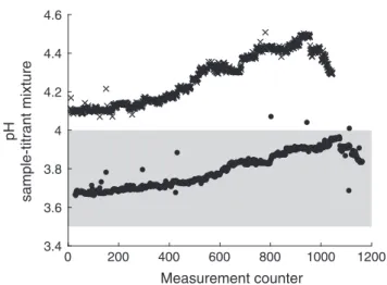
Figure 6 illustrates the possibleATworking range as a function of the pH of the sample-titrant mixture observed with analyzers using spectrophotometric pH measurements with BCG. In this figure, theATworking ranges of the red and the gray system are based on the resulting pH working range observed with the MSM 68/2 underway measurements (pHminto pHmax,seeFig. 7).

On the one hand, the configuration of the red system yields in a wider measurement range, where small pH steps correspond to largerATsteps, which makes it more attractive for regions with highATvariability. On the other hand, the gray system is more precise due to larger pH steps corresponding to smallerATsteps.

To take advantage of this better precision, the choice of a higher pH range (4.0–4.5) is more useful for regions, where small AT

changes are expected.

Another potential problem with pH ranges above 4.0 is the unknown validity of the AT calculation following Eq. 7 (see

“Materials and methods”section). Li et al. (2013) only validate this calculation within pH values of 3.5–4.0. In this range, the concentrations of the terms ½H3PO4, B OHð Þ4⁻

, ½OH⁻, HPO²₄⁻

, PO³⁻₄

, SiO OHð Þ3⁻

, NH½ 3,and HS½ ⁻ can be neglec- ted. Following the calculation procedure of Li et al. (2013), recalculation of these concentrations at higher pH values results in an overall increase of the corresponding alkalinity contributions from approximately 0.4μmol kg⁻¹ at pH 4.0 up to approximately 0.9μmol kg⁻¹at pH 4.5, and, consequently,

in an increase in the systematic error of the method. However, it has to be noted that the total concentrations of these species, on which the calculation of Li et al. (2013) is based, are much higher than those of typical open ocean seawater (worst-case scenario). Based on this fact, it can be assumed that the concen- trations of the above listed terms can still be neglected within the given instrument uncertainties, thus Eq. 7 is also valid up to a pH of 4.5. Additionally, laboratory performance tests simi- lar to that in “Laboratory experiments” section with another CONTROS HydroFIA^®TA system (similar configurations to the gray system, but no leakage) support thisfinding. There, a lin- ear slope of (1.010.01), and (1.0000.003) measured with a maximum pH of 4.6, and 4.3, respectively, was observable (data not shown), which indicates unbiased performance of the system. Just an increase of the RMSE with increasing pH is detectable (ΔRMSE = 1.8 μmol kg⁻¹). The found decrease in accuracy at those high pH values can be explained by the limit of the spectrophotometer’s ability determining the very low concentrations of the remaining indicator acid. Because of that, it is not recommended to measureA_Tat pH values greater than 4.6.

Performance characteristics

In this part, only the performance characteristic of the red analyzer during the MSM 68/2 cruise is shown and discussed.

Because it had no malfunctions during its deployment, these results are representative for the behavior of the system as such.

For evaluating precision, the standard deviation σ (n = 5) of each repeated CRM measurement was determined. Figure 8 shows these standard deviations as a function of the measure- ment counter. The averaged field precision is determined at 1.2 μmol kg⁻¹. For an autonomous system, such a level of

3.5 4 4.5 5

pH of sample-titrant mixture Possible AT working range

Fig. 6.PossibleATworking range as a function of the sample-titrant mix- ture pH. The red and the gray area indicate the measuredATrange of the red and the gray system, respectively, during the cruise MSM 68/2. The vertical dashed lines indicate the optimal pH range of 3.5–4.0 given by Breland and Byrne (1993) and Li et al. (2013).

0 200 400 600 800 1000 1200

Measurement counter 3.4

3.6 3.8 4 4.2 4.4 4.6

pH sample-titrant mixture

Fig. 7. pH of the sample-titrant mixture (after degassing) of the MSM 68/2 underway measurements as a function of the measurement counter, wherefilled circles and crosses represent the red and the gray system, respectively. The gray area indicates the optimal pH range of 3.5–4.0 given by Breland and Byrne (1993) and Li et al. (2013).

precision is in good agreement with the requirements of Dickson et al. (2007) as stated for standard AT titration methods for which a standard deviation of better than 1μmol kg⁻¹is required.

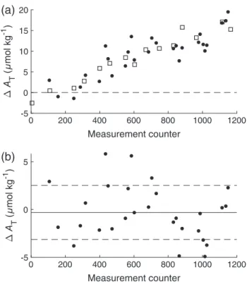
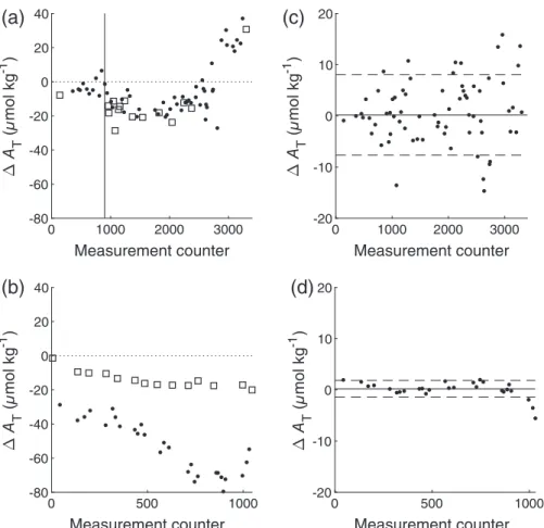
For evaluating accuracy, the bias (ΔAT=AT,Analyzer−AT,Reference) between the analyzerATmeasurements and theATvalues of the reference samples is calculated. Figure 9 shows the biases of the red system as function of the measurement counter both with raw data (Fig. 9a) and with linearly drift corrected data (Fig. 9b). This correction is necessary, because the analyzer shows a linearly increasing ΔAT from −2 μmol kg⁻¹ at the beginning up to +15μmol kg⁻¹at the end of the cruise. The conducted CRM mea- surements are used for this drift correction resulting in a mean bias of−0.32.8μmol kg⁻¹(n= 28) between the red system and the reference data from discrete samples measured by standard open- cell titrator (including the sampling error). Such a level of accuracy is comparable to standardATtitration methods. Furthermore, by plotting theATvalues of the analyzer (already corrected against the drift using the CRM measurements) against the referenceAT

values, the linear function y = (0.980.01)×x+ (4023) (R²= 0.997) results. Taking all uncertainties in account, this result proofs the good sensitivity of the analyzer over the whole working range.

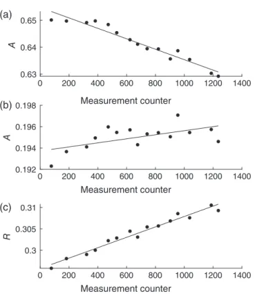
We discovered that the observed linear drift with increasing measurement number occurs because of material deposits in the optical pathway. As a result, the light intensity decreases and therefore the absorbanceAat 444 and 616 nm changes.

Usually, such an intensity loss is corrected by the dark and blank spectrum within the measurement routine, but the opti- cal measurements showed systematic deviations over time at the different wavelengths. Figure 10 shows the absorbance changes at 444 and 616 nm of the red system’s CRM measure- ments in dependence of the measurement counter during the MSM 68/2 cruise, and also the resulting change in the absor- bance ratio R. Theoretically, the absorbance ratio of a CRM measurement should not change, provided the same batch is

measured. In reality, Fig. 10c proves that this is not the case.

R increases over time due to the different behavior of the absorbances at 444 and 616 nm, and an increasingRleads to increasing AT values. We hypothesize that the deposits are caused by colored substances, possibly by a decomposition of the BCG indicator or impurities, which cannot be completely prevented at the moment. Consequently, the observed linear drift toward higher AT values has to be accepted as typical behavior. Fortunately, the drift can be easily corrected for by regular reference measurements. Even by applying one refer- ence measurement in the beginning and one in the end of a deployment in our case would have been sufficient because of the linear character of the drift.

Recent results from other deployments show a similar drift magnitude but over a much longer time period with lower measurement interval of 90 min. Consequently, a small resid- ual deposit is left on the optical window after each measure- ment leading to accumulation over time as a function of number of measurements. This indicates that this pattern is related to the number of conducted measurements (number of indicator injections) rather than the pure deployment time.

0 200 400 600 800 1000 1200 1400 Measurement counter

0 0.5 1 1.5 2 2.5 3

(µmol kg-1 )

Fig. 8.Standard deviationσof repeated CRM measurements as a func- tion of the measurement counter of the red analyzer during the cruise MSM 68/2. The horizontal black line indicates the averaged standard deviation.

0 200 400 600 800 1000 1200

Measurement counter -5

0 5 10 15 20

A T (µmol kg-1 )

0 200 400 600 800 1000 1200

Measurement counter -5

0 5

A T (µmol kg-1 )

(a)

(b)

Fig. 9. (a) Bias plot for the intercomparison of AT measurements between the red analyzer and the reference samples during the cruise MSM 68/2, where open squares represent the CRM and filled circles represent the discrete samples measured with the standard open-cell titrator in the laboratory. The horizontal dashed line indicates ΔAT= 0μmol kg⁻¹. (b) Bias plot (discrete samples) after a linear drift cor- rection using the CRM measurements. The horizontal black line indicates the mean bias, ΔAT, while the dashed lines indicate ΔAT σ (for this data set:−0.32.8μmol kg⁻¹).

For approximating the combined standard uncertainty infield, the daily CRM measurements were used. The precision of each repeated CRM measurement was utilized as random uncertainty component, and the root mean square of the biases to the certified value of the measured CRM (ΔA_T=A_T,CRM−A_T,Analyzer) as system- atic uncertainty component, respectively. Additionally, the uncer- tainty contribution of the drift correction to the systematic uncertainty was estimated and implemented by using the RMSE of the linear regression. The relative combined field standard uncertainty of the analyzer was estimated with 0.10% at 2212.44μmol kg⁻¹(certified value of CRM Batch No. 160). Due to the proven linearity of the analyzer over the working range of 2000–2450μmol kg⁻¹, the combinedfield standard uncertainty is estimated with 2.0–2.5μmol kg⁻¹(seeSupporting Information for more information). Thisfield uncertainty approximation is in full agreement with the“weather”goal requirements of Newton et al.

(2015). The very high requirement of the“climate”goal is almost be achieved in thefield by being only 0.5μmol kg⁻¹higher than the target of 2μmol kg⁻¹. Thus, thefield standard uncertainty of the analyzer is sufficient for ocean acidification measurements.

Long-term precision

The result of the long-term precision experiment during the M 133 cruise is shown in Fig. 11. The standard deviation of the long-term measurements is determined with 2.4 μmol kg⁻¹

(n= 178), which is higher than the averaged short-term preci- sion of1.2μmol kg⁻¹observed with the red analyzer during the MSM 68/2 campaign. This reduced precision is due to the instrument long-term drift, and changes of the environmental or sample conditions, that was already reported in the over- lapping Allan experiment results. Unfortunately, it has to be mentioned that this experiment was carried out after the leak- age in the degasser unit appeared. A functional analyzer would probably show better results. However, while long-term stan- dard deviation of2.4 μmol kg⁻¹does not reach the require- ments for standard open-cell titrators, it still is in an acceptable range. Another outcome of this experiment is the appearance of outliers. Overall, 11 outliers are recognizable in the data set, which is 6.2% of the measurements. This outlier rate seems to be relatively high, but, especially during long-term deploy- ments, the measurement resolution of the CONTROS Hydro- FIA^® TA system (measurement time per sample: < 10 min) is high enough to compensate these outliers. Additionally, remov- ing these outliers using an algorithm (e.g., Grubbs outlier test by Grubbs 1974) is very well possible during the post- processing, since appear as spike outliers in the regular data set.

The reasons for the occurrence of these outliers are still unclear.

We hypothesize that the sample pump supplies a minimally higher volume of seawater to the sample loop than usual. In addition, bubbles in the sample loop could be possible.

Initial drift after idle time

Figure 12 shows the results of the initial drift experiment during the M 133 cruise. After the veryfirst start of the system following an idle time of approximately 3 months, the required 0 200 400 600 800 1000 1200 1400

Measurement counter 0.63

0.64

(a) 0.65

(b)

(c)

A

0 200 400 600 800 1000 1200 1400 Measurement counter

0.192 0.194 0.196 0.198

A

0 200 400 600 800 1000 1200 1400 Measurement counter

0.3 0.305 0.31

R

Fig. 10.AbsorbanceAat the wavelengths of the indicator absorption maxima (a) 444 nm, and (b) 616 nm of the CRM measurements with the red system as a function of the measurement counter during the MSM 68/2 cruise. (c) Absorbance ratio R (R = A616nm/A444nm) of these CRM measurements as a function of the measurement counter.

0 50 100 150

Number of measurements 2330

2340 2350 2360 2370 2380 2390 2400

AT (µmol kg-1 )

Fig. 11.ATlong-term measurements of a stable seawater substandard as a function of the measurement counter of the red system during the cruise M 133, wherefilled circles indicate the regular measurements, and open circles the outliers in this data set (Grubbs outlier test,α= 0.05, two-sided, n= 178). The horizontal black line represents the resulting meanATvalue, AT, without outliers. The dashed black lines indicateATσ.