SFB 649 Discussion Paper 2012-024
Bye Bye, G.I. - The Impact of the U.S. Military
Drawdown on Local German Labor Markets
Jan Peter aus dem Moore*
Alexandra Spitz-Oener*
* Humboldt-Universität zu Berlin, Germany
This research was supported by the Deutsche
Forschungsgemeinschaft through the SFB 649 "Economic Risk".
http://sfb649.wiwi.hu-berlin.de ISSN 1860-5664
S FB
6 4 9
E C O N O M I C
R I S K
B E R L I N
Bye Bye, G.I. - The Impact of the U.S. Military Drawdown on Local German Labor Markets
∗Jan Peter aus dem Moore1 and Alexandra Spitz-Oener2
1Humboldt-Universität zu Berlin
2Humboldt-Universität zu Berlin, IAB, CASE, IZA
March 2012
Abstract
What is the impact of a local negative demand shock on local labor markets? We exploit the unique natural experiment provided by the drawdown of U.S. military forces in West Germany after the end of the Cold War to investigate this question. We nd persistent negative eects of the reduction in the U.S. forces on private sector employment, with con- siderable heterogeneity in terms of age and education groups, and sectors. In addition, the U.S. forces reduction resulted in a rise in local unemployment, whereas migration patterns and wages were not aected.
Key Words: Labor demand shock; Base closure; Employment; Wages JEL Classication: J23, R23
∗This research was supported by the Deutsche Forschungsgemeinschaft through the SFB 649 Economic Risk. The authors thank Michael Burda, Rene Fahr, Bernd Fitzenberger, Jochen Kluve, Michael Kvasnicka, Guy Michaels, Enrico Moretti, Regina Riphahn, seminar and conference participants at Humboldt University Berlin, Albert-Ludwigs-University Freiburg, the University of Paderborn, the GfR-IAB conference in Dresden, the CRC649 conference 2011 in Motzen, the 10th Brucchi Luchino Labor Economics Workshop at the Bank of Italy in Rome, the 5th RGS Econ Conference in Duisburg as well as members of the Berlin Network for La- bor Market Research (BeNA) for very helpful discussions and comments. The labor market data used in this paper were obtained from the Institut für Arbeitsmarkt- und Berufsforschung (IAB). We thank Stefan Bender, Tanja Hethey-Maier and Stefan Seth for invaluable help with the data. Andreas Andresen, Cindy Lamm and Jessica Oettel provided excellent research assistance. The sole responsibility for the analysis and interpretation of the data in the paper remains with the authors. Corresponding author: Alexandra Spitz-Oener; E-mail:
alexandra.spitz-oener@wiwi.hu-berlin.de.
1 Introduction
The impact of economic shocks on local labor markets is a subject of long-standing interest to economists, policy makers and the general public alike. In particular, the nature and magnitude of potential local consequences of economic shocks are important for the justication and design of regional economic policies. In many countries, considerable resources have been devoted to helping regions mitigate and overcome past adverse economic shocks or to attracting new investment in the hope of positive local externalities. Despite this interest, empirical research has had diculty establishing the causal eects of local economic shocks.1
In this paper we identify the causal eect of a local economic shock by taking advantage of a shock that induced large exogenous shifts in labor demand in several districts of four states (Bundesländer) in West Germany, but not in others. Specically, we exploit the district variation in the stationing and withdrawal of U.S. military forces in Germany after German reunication and the end of the Cold War to examine the consequences of regional economic shocks on local private sector employment. In addition, we also investigate the impact of this labor demand shock on wages, unemployment and migration.
The unique natural experiment setting of the event allows us to improve on limitations that impaired previous studies analyzing the eect of regional economic shocks on local labor markets.2 The U.S. forces were stationed in West Germany in the 1950 at strategic points along two major defense lines; local economic considerations were not important in this decision process. In addition, and in a similar fashion to the stationing decision, the withdrawal decisions for the U.S. forces in Germany were made exclusively by U.S. military ocials and were neither subject nor responsive to any politicizing: the U.S. Department of Defense decided on the details of the withdrawal process purely on strategic military grounds. Both of these facts alleviate concerns regarding the validity of exogeneity assumptions.
The U.S. forces aected the German local economies through three main channels: rstly, the bases demanded goods and services from German companies; secondly, the U.S. soldiers, civilian employees and their dependents were consumers in the local economies; and thirdly, the
1See Moretti (2011) for a recent review.
2It also allows us to improve on limitations that previous studies on the eects of base closures faced. For example, the Base Realignment and Closure Process (BRAC) in the U.S. and the realignment of the German Army are both likely to be inuenced by strong local or regional stakeholders lobbying to safeguard their bases against closures.
bases acted as employers of German civilian workers.
Although German civilian employees typically comprised a small fraction of local employment (the median is less than 0.5 percent of local employment in districts with U.S. military presence in 1989), many of the early studies were preoccupied with the fate of these German employees.3 This focus reects in part the overriding public and political interest at the time and the fact that the legal status of the local national employees was then unclear.4
We focus on eects that are mainly driven by changes in channels one and two: at the end of the 1980s, there were about 250,000 U.S. servicemen stationed in Germany (see Figure 1).
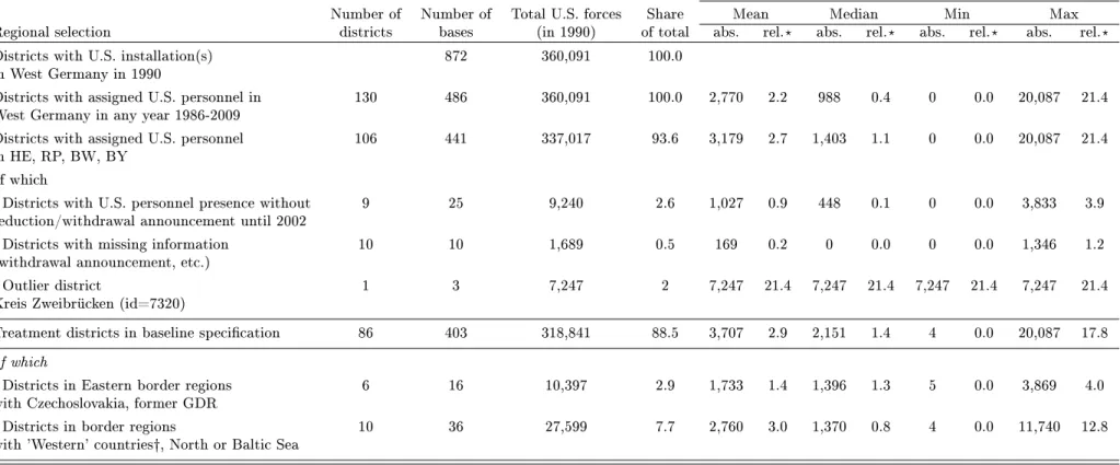
Together with the U.S. civilians whom the bases employed and the family members they all brought along, the total U.S. presence in West Germany amounted to nearly 600,000 persons in 1989 (see Figure 2). At the district level where the U.S. bases were located, the U.S. presence was sometimes large; for the 86 districts with a U.S. presence retained in our baseline anal- ysis, the mean of the U.S. force level in 1990 was 3,707, which represents 2.9 percent of the district population.5,6 The U.S. forces consumed mainly local, non-traded goods and services from German sources with respect to traded goods and services, the U.S. bases were mostly self-sucient. Overall, the withdrawal process represented a large consumption shock to the aected regions which translated into a negative shock to local labor demand.
The results indicate that the realignment of the U.S. forces did indeed have signicant nega- tive eects on local private sector employment in Germany. On average, our coecient estimates suggest that the complete withdrawal in a given district is associated with a 0.4-0.7 percent year- by-year drop in the number of jobs in the local private sector. An analysis of the dynamic pattern
3See, for example, Blien et al. (1992), Blien (1993), and Gettmann (1993).
4See, for example, the ocial information requests by members of the German parliament (Deutscher Bun- destag, 1990a,b,c, 1991a,b) and the report by the U.S. General Accounting Oce (1992) on the process of reducing the local national workforce.
5See Table 1. U.S. military deployments abroad of comparable size have only recently been built up in Afghanistan and Iraq, with the peak of the force levels totaling 42,500 (about 0.1 percent of the local national population) in Afghanistan and 251,100 (about 0.8 percent) in Iraq in 2009 (for the force level data, see Belasco (2009); the population data for the relative importance of the deployments has been sourced from the Cen- tral Intelligence Agency (2011)). A new report for the U.S. Senate Foreign Relations Committee (U.S. Congress, 2011) discusses whether Afghanistan might be infected by a "Dutch Disease", i.e. an overdependence of local employment on foreign aid connected to the foreign troop presence that might vanish into thin air in the case of a swift withdrawal. We do not argue that our estimates for the drawdown in Germany could be extrapolated to these cases as the circumstances of the deployments, the level of development of the countries, and the base structures and relationships with the local economy are vastly dierent.
6Bebermeyer and Thimann (1990) attempt to assess the aggregate economic importance of the US stationing in West Germany using a cost-benet balance sheet accounting approach. Combining various data sources from 1986 and 1987, they calculate an annual gross benet of 14.8 billion German DM and a net benet (subtracting cost items that are largely borne by the German federal budget) of 12.5 billion DM, which is equal to 0.62 per cent of the West German gross national product at the time.
reveals that this adverse eect is persistent and does not fade away even several years after the withdrawal shock rst hits. In line with the specics of the consumption shock on which we are focusing, the employment eects are most pronounced for local goods and services sectors that were prone to suer most from the reduction of local purchasing power, and were primarily borne by young and old, and by low- to medium-skilled workers. We also nd evidence of a rise in local unemployment, whereas we do not nd eects along the migration margin or in terms of local wages.
This study advances the literature on the consequences of economic shocks on local labor markets. The traditional approach in the literature uses deviations in regional time series of employment from national averages to investigate the consequences of economic shocks (for ex- ample, Topel, 1986, Decressin and Fatas, 1995) and Blanchard et al. (1992) in part of their analysis). Employment, however, is determined by both labor demand and supply forces, and these studies are not able to identify the eects of these two factors separately. Another promi- nent approach in this area of the literature is to identify local economic shocks by using national changes in industry employment interacted with measures of local industrial composition (see, for example, Bartik, 1991, Blanchard et al., 1992, Bound and Holzer, 2000, Moretti, 2010, and Notowidigdo, 2011). While this instrument is likely to be exogenous to local labor supply, it is not clear whether it captures shocks to local labor demand very well. It is possible, for example, for a region to lose employment in an industry even though that industry is growing on the national level.
Carrington (1996) was among the rst studies to examine a specic shock, namely the construction of the Trans-Alaska Pipeline System (TAPS) between 1974 and 1977. He analyzes how this construction project aected the Alaskan labor market and nds that the timing of the evolution of aggregate monthly earnings and employment closely matched changes in TAPS- related activities. Overall, however, the ndings suggest that this major demand shock had only short-term consequences for the Alaskan labor market.
Other studies involving specic shocks use variation in energy prices to analyze the impact of labor demand shocks on local labor markets. Black et al. (2005a), for example, analyze the impact of the coal boom and bust in the 1970s and 1980s on local labor markets and nd positive eects of the boom on local non-mining sector employment and earnings, in particular in non-
mining sectors producing local goods.7 The coal bust led to negative eects that are smaller than the positive eects during the boom.8 They also nd that the regions aected by the coal bust experienced considerable population losses, whereas population growth was barely aected by the coal boom. Studies that identify shocks through price uctuations in natural resources such as coal or oil focus on price changes of input factors that are widely used throughout the economy; it is unlikely that these price uctuations only impact on the energy-extracting industries and do not have repercussions on both non-energy-extracting industries within the treatment regions and industries outside these regions, in particular as prices of dierent energy resources are highly correlated.
A common feature of the analysis by Carrington (1996) and the studies focusing on energy price uctuations is that they analyze shocks to very isolated or mainly rural regions,9 and some of the results might be explained by these idiosyncrasies (e.g. that population growth in the resource-rich regions was not aected by the coal boom in Black et al., 2005a). None of the districts in the four West German states under consideration are as rural or remote as the regions of main interest in these earlier studies.10
Our analysis also diers from these earlier studies with respect to the time frame. In the setting of all these studies, the economic actors should have been aware of the fact that the shocks were not permanent. We focus instead on a permanent and irretrievable shock that should have been perceived as such by the economic agents. In this respect, our study is similar to Greenstone and Moretti (2003) and Greenstone et al. (2010), who study the regional industry- level employment and productivy eects from the awarding of "Million Dollar Plants". While their analysis provides an original identication design for regional spill-over eects by focussing on the dierent evolutions in "winner" and "loser" counties in competitive biddings for large industrial plants, an important limitation of their data is that it does not provide information on the expected size of the plant, which is likely to be important for the magnitude of the potential
7For a similar analysis using Canadian data see Marchand (2011).
8In other papers, these authors investigate how the coal boom and bust aected other outcome variables such as education or participation in disability programs (Black et al., 2002, 2003, 2005b).
9Alaska is obviously very remote; but Kentucky, Ohio, Pennsylvania and West Virginia, the states in which treatment and control districts are located for the analysis by Black et al. (2005a), are also rural areas with population density ranging from 30 - 110 inhabitants per square kilometer.
10Several studies consider other arguments as to why adjustments to economic shocks might play out dierently;
factors discussed include relative skill supply, the enterprise ownership structure or the housing supply in the aected regions. See, for example, Bound and Holzer (2000), Glaeser and Gyourko (2005), Kolko and Neumark (2010), Notowidigdo (2011), and Larson (2011).
spill-over eects into employment and welfare. The U.S. withdrawal process on which we focus is a well-dened shock because the data at hand allow us to measure precisely the size and structure of the shock for all treatment areas.
The paper is structured as follows: the next section provides a brief account of the historical background of the stationing and withdrawal of the U.S. military forces in Germany. In Section 3 we present our estimation strategy, and Section 4 discusses the data. Section 5 reports our results, separately for regional employment, wages, unemployment and net migration, as well as several robustness checks. Section 6 provides a conclusion.
2 Historical Background
2.1 U.S. Forces in Germany 1945-1990
After the end of World War II, the Allied Forces (American, British, French and Soviet) es- tablished four occupation zones in Germany. Following negotiations that had already started during the war in 1944 within the allied European Advisory Council (EAC) and that had been agreed upon in principle at the Yalta conference, the nal demarcations of the 4 zones were conrmed by the Potsdam Agreement on August 2, 1945.
The American zone included a large part of the southwest area of Germany (which was later to become the states of Bavaria, Hesse, and the northern part of Baden-Württemberg) plus the seaport town of Bremerhaven on the North Sea and the American Sector in Berlin. In Article 12 of the "Berlin Declaration" issued on June 5, 1945, the Allied Powers granted themselves the authority "to station forces and civil agencies in any or all parts of Germany as they may determine" (U.S. Department of State, 1985). However, there were initially no plans for a major permanent military presence. With the burgeoning confrontation of the Cold War marked by the establishment of two states on German soil in 1949, the Berlin blockade and airlift, and the war in Korea, the Western Allied Powers established NATO (which the West German Federal Republic of Germany (FRG) joined in 1955) as a common defense organization and deterrent against potential Soviet aggression. The NATO "Forward Strategy" foresaw the West German area as the central battleeld where a potential Soviet invasion would have to be halted until additional forces could be activated. Against the backdrop of this concept, the U.S. forces in Germany established bases at strategic points along two major lines of defense, expanding their
presence also beyond the early boundaries of the American zone.11
An estimated number of 1.9 million American soldiers were stationed on German soil at the end of World War II.12 After the temporary reduction to less than 100,000 in the rst years of the occupation up to 1950, the strength of the U.S. forces was consolidated to around 250,000 in the mid 1950s. Figure 1 tracks the historical evolution of the U.S. active military personnel in Germany from 1950 to 2005. Apart from some temporary build-ups and reductions, for example after the Berlin and Cuban Missile crises in the early 1960s and later due to the Vietnam War, the level of the American military presence remained more or less stable until 1989, making it one of the largest and longest peace-time deployments of an army in a foreign country in modern history.13 The overall U.S. presence, including the employed civilian personnel and dependents was even more signicant, totaling more than 570,000 in the spring of 1989 (see Figure 2). The U.S. forces in Germany maintained over 800 bases and installations, ranging from small unmanned signal posts to training areas covering more than 20,000 hectares or airbases that employed more than 12,000 personnel. The left part of Figure 3 illustrates the regional distribution and the relative personnel size of the U.S. bases across Germany in 1990.
2.2 The Withdrawal and Realignment of U.S. Forces after 1990
The end of the Cold War created a turning point for the U.S. presence in Germany. In March 1989, the NATO countries and their counterparts from the Warsaw Pact began negotiations on reductions of conventional armed forces in Europe. The fall of the Berlin wall on November 9, 1989 and the swift political transformations in several Eastern European states further sped up the negotiations, and just one month after the formal reunication of Germany, the Conventional Armed Forces in Europe (CFE) treaty was signed in November 1990.
Several ocial U.S. government reports (U.S. General Accounting Oce, 1991a,b) and the comprehensive study conducted in 1995 by the Bonn International Centre for Conversion (BICC) (Cunningham and Klemmer, 1995) provide detailed insights into the planning and exe-
11Several large airbases were constructed, for example, in Rhineland-Palatinate in the former French occupation zone west of the Rhine considered to be less vulnerable to a Soviet attack. For a brief account of the history of U.S. forces in Germany, see for example Duke (1989), pp. 56-148. For details on the U.S. base planning in Rhineland-Palatinate, see van Sweringen (1995).
12See Frederiksen (1953) and Trauschweizer (2006).
13The numbers in Figure 1 also reveal the distribution between the dierent branches of the U.S. armed forces, with the Army constituting 70-85 percent, the Air Force 10-30 percent and the Navy and Marine Corps less than 1 percent of the total deployment at any point in time.
cution of the U.S. drawdown process. In preparation for some of the structural changes that were to materialize in the future, the European command of the U.S. Army in Europe (USAREUR) had formed a planning group as early as July 1988. Based on the troop ceilings established in the CFE negotiations, the USAREUR command was quick to draw up a plan to recongure the required force levels and identify units for withdrawal and bases and communities for closure.
The key criteria for the selection of sites by U.S. military ocials were
(i) "ensuring that the forces would meet military and operational requirements;
(ii) decreasing support costs and increasing eciency of base operations;
(iii) minimizing personnel moves;
(iv) reducing environmental impact; and
(iv) considering the proximity of training areas, the quality of housing and facilities, the local political and military environment, the concerns of host nations, and the base's proximity to road and rail networks."14
On September 18, 1990, the Pentagon publicly announced the closure and realignment of 110 sites in Germany, starting the rst phase of the withdrawal.15 By 1996, another 20 rounds of base closures in Germany would be gradually announced, bringing the number of U.S. military personnel at the end of the 1996 scal year to a low point of around 85,000, a massive 75 percent reduction compared to the 1989 level. Although the ocial documents and newspaper accounts from the time mention some coordination between U.S. and German authorities, they also high- light the fact that the local German politicians and communities were usually taken by surprise and learned about the imminent closures only around the time of the public announcements by the U.S. forces in the news media.16,17 The "drawdown shock" at the local level was further
14U.S. General Accounting Oce (1991b), p.3.
15Earlier, U.S. Defense Secretary Dick Cheney had already announced the closure of Zweibrücken air base in Germany on January 29, 1990, as part of a round of mostly domestic base closures within the 1991 scal year defense budget (Doke, 1990; Vynch, 1990).
16Cunningham and Klemmer (1995) describe how the US Department of Defense maintains complete author- ity which has to a large extent de-politicized the foreign base closure process compared to the domestic BRAC process. They report that even for Rhineland-Palatinate, where the state authorities specically requested that the United States close primarily installations in densely populated and highly industrialized urban areas (...), but keep open the sites located in rural and underdeveloped areas of the state, these priorities were inconse- quential due to the increasing pace of the withdrawal. They conclude as follows: In none of the cases reviewed were the German civil authorities able to stop or reverse the US decision to withdraw. In some limited cases (...) German ocials were able to delay closure. Conversely, some high-level requests to delay closure were denied.
17We conducted an extensive newspaper archive search of both U.S./international and German newspapers (including, but not limited to major titles such as Business Week, The Economist, The Wall Street Journal, Der SPIEGEL, Frankfurter Allgemeine Zeitung (FAZ), Süddeutsche Zeitung (SZ), Handelsblatt as well as Stars
exacerbated by the short time frame of 180 days that the U.S. forces envisaged between the announcements and the completion of the withdrawals with the return of the vacated sites to German authorities.
With the U.S. troop levels reaching new target levels of around 90,000 and new safety threats emerging in Europe (for example in the Balkans after the dissolution of Yugoslavia), the pace of the drawdown process slowed down considerably in the mid-1990s. Only after the terrorist attacks of 2001 that resulted in a comprehensive redesign of U.S. security policy, including changes in overseas basing, were new rounds of major U.S. base closures in Germany announced and implemented. This process is still underway: in summer 2010, USAREUR announced a major withdrawal by 2015 from the Heidelberg and Mannheim area, a former stronghold and location of the headquarters of the U.S. Army in Germany.18
In summary, three features of the stationing and drawdown process deserve highlighting, as they lay the foundation for the identication strategy in the empirical analysis. Firstly, both the designation of the initial U.S. base locations after the occupation, but even more importantly, the base closure and realignment decisions half a century later, were governed unequivocally by American strategic military considerations. Secondly, local withdrawals of the U.S. forces constituted abrupt socks with a surprise element for agents in the local economy. Thirdly, the magnitude of the withdrawal process was large and exhibited strong variation in size and timing at the local level.
3 Empirical Approach and Identication
We identify the causal eect of the U.S. withdrawal on local labor markets by estimating dierence-in-dierence (DD) models, contrasting the evolution of employment and wages in dis- tricts with a U.S. presence and subsequent withdrawal and a group of control districts. In our simplest specication for employment, the empirical model estimated by OLS has the following
& Stripes, the major news outlet for the U.S. military community) for the years 1988 to 2009, either via the news archives of the respective media and/or comprehensive databases such as Factiva and Genios. Based on alternative search keywords such as U.S. Army, U.S. Forces, bases, closures, realignment and Germany, the articles that we found in all cases relayed (if any) specic information about the locations, extent and timing of drawdown decisions only after the fact, i.e. after the information had already been ocially disclosed by the U.S. Department of Defense and/or the U.S. forces in Germany. A bibliography of all the articles found is available from the authors upon request.
18The latest piece of information in this respect appeared in the New York Times on January 12, 2012, announcing that the U.S. will withdraw another brigade (about 4,000 soldiers) from Germany, as the new military strategy focuses on the Asia-Pacic region and on sustaining a strong presence in the Middle East.
form:
(1) logYkt=αk+δt+β×logU.S. Forceskt×1[t>Y ear0k]) +kt
The dependent variables are district-level measures of employment, denoted by Y, in district k and year t. The parameter of interest, β, is the coecient on the logarithm of the level of U.S. forces in the given district k in year t, and an indicator function for the post-treatment period that varies according toY ear0k, the year of the rst announcement of a U.S. withdrawal in a given treatment district. All estimates include a vector of district dummies, αk, that control for mean dierences in employment across districts, and year dummies, δt, that adjust for employment growth common to all districts. So β reects the extent to which employment growth in a district varies with the extent of the U.S. forces reduction.
In extensions to the specication of Equation 1, we estimate specications that include dummies for state-by-year, and linear or quadratic district-specic time trends in order to allow for deviations from the common trend assumption. In the latter, the identication of the eects of U.S. withdrawal comes from whether the withdrawal lead to deviations from preexisting district-specic trends.19
For the analysis of the wage outcomes that vary at the individual level, we augment speci- cation (1) with covariates that control for individual characteristics:
(2) logWikt=αk+δt+β×logU.S. Forceskt×1[t>Y ear0k]) +Xiktγ+ikt,
where the subscript i denotes the individual observations. The vector of individual controls, Xikt, includes a quartic in age and dummies for foreign citizenship, occupations, and industries.
In order to capture potentially heterogeneous treatment eects according to industry, we perform both pooled estimations across all industries and separate estimations using industry- district samples. Again, all models are estimated in extensions that include state-by-year dum-
19In our baseline estimations, we do not weight the district-year observations in any way for two reasons:
rstly, as the employment data is summarized from the full universe of establishments, there is no systematically heteroscedastic measurement error that varies with the district size. Secondly, since we are interested in the average "treatment" eect of the U.S. withdrawal in a district, there is no specic reason to place more weight on large districts. See Autor (2003) who puts forward these arguments in his analysis of the eect of exceptions to the common dismissal law on temporary help service employment growth in U.S. states. Moreover, if we do weight the observations by district population, the results - as reported in one of the later robustness checks and available in detail from the authors upon request - are virtually unchanged from the unweighted results.
mies and linear or quadratic time trends.
In the recent applied econometrics literature, two potential problems for the consistent es- timation and inference in DD models have received considerable attention. Firstly, Bertrand et al. (2004) show that the inference based on the standard treatment of clustered errors can be misleading in the presence of serial correlation. They demonstrate that next to more complex approaches such as block bootstrap methods20, the bias in the standard errors can be reduced to viable levels by clustering at the group level if the number of groups is suciently large for asymptotic theory to hold. Secondly, following up on seminal contributions by Moulton (1986, 1990), Donald and Lang (2007) report that the standard methods for dealing with a DD model that mixes individual and group-level data and where the regressor of interest varies only at the group level also suer from severely downward-biased standard errors in the presence of intra- group correlations. In our context, we address these concerns by following the recommendations by Angrist and Pischke (2009, chap. 8): in our baseline employment and wage estimations, we use Huber-White robust standard errors clustered at the district level to allow for arbitrary forms of correlation within districts and rely on the large number of districts and time periods in our setting.21 For our wage estimations, where we face the Moulton problem, we further conrm the robustness of our results by implementing a two-step estimation procedure as pro- posed by Donald and Lang (2007) that rst aggregates on the group level and then performs the DD estimation on covariate-adjusted district averages.22 Finally, in some of our robustness checks, we also show that our results are robust if we implement an alternative two-way cluster- ing method recently suggested by Cameron et al. (2011) or cluster standard errors at the higher aggregation level of labor market regions to allow for spatial autocorrelations across districts within the same labor market region.
4 Data and Descriptive Evidence
We consider employment and wage outcomes from 1975 to 2002 for 202 districts (NUTS-3,
"Landkreise und kreisfreie Städte") that are located in the four German federal states of Hesse,
20See, for example, Fitzenberger (1998), Conley (1999).
21Although the minimum required number of clusters cannot be easily determined as it depends on the appli- cation, Angrist and Pischke argue that the evidence from DD research on U.S. states suggests that more than 50 clusters should be sucient. In our baseline setting, we use a total of 182 districts with 86 in the treatment and 96 in the control group.
22The results from these estimations are available upon request.
Rhineland-Palatinate, Baden-Württemberg, and Bavaria. More than 95 percent of the U.S. Mil- itary personnel was based in these states in 1990, that is before the beginning of the drawdown.
Our treatment variable is a measure of the annual level of U.S. forces in a given district.
The data on the regional level of U.S. forces are calculated from a newly constructed database that combines ocial U.S. data on the number of assigned personnel at the individual base level with the geocoded location of the base and the dates when realignment and closure decisions were rst announced. Details on the original U.S. military data sources and the construction of the database are provided in the Data Appendix. Figure 3 illustrates the extent of the base realignments between 1990 and 2002 across West Germany, while Table 1 shows the selection of the districts and Figure 4 shows the distribution of the U.S. forces for the treatment districts in 1990. The mean (standard deviation) of this variable is 3,707 (4,477), the median is 2,151 and the min (max) is 4 (20,087). Districts within the four southern federal states in which the U.S. Military was never present constitute the control group. Figure 5 exhibits the geographical distribution of the 86 treatment and 96 control districts in our baseline sample.
Data on our outcome variables of employment and wages for all districts in our sample is based on the full universe of the social security records which are provided by the German Institute for Employment Research (IAB). The individual employment spells, drawn from the entire set of employment histories (Beschäftigten-Historik, BeH ), provide information on the employees' characteristics (for example, age, nationality, and education) and with the use of an employer identier for each spell, are merged with rm-level information from the histories of es- tablishments (Betriebs-Historik-Panel, BHP) that detail the industry aliation, and workplace location. Our outcome data is thus very similar to the variables contained in the IABS, a widely used and well documented 2% subsample of the social security records that is publicly available to researchers.23
The use of the full universe of the employment spells is crucial to our analysis. We expect that the eects from the military drawdown primarily accrue to employees of small and medium- sized companies that are active in local non-tradable industries. Using the IABS directly for the analysis would therefore not be a suitable alternative, since employment spells from employees in large rms and/or large industries are more likely to be included there.24
23See the latest IABS data documentation in Drews (2007).
24See Dustmann and Glitz (2008) for a similar argument in the context of rm-level responses to changes in local labor supply. They report that for 1995, the share of large rms with more than 100 employees included in
The data include all employment that is subject to social security contributions, but ex- cludes the self-employed, civil servants, students enrolled in higher education, and the German military. More importantly for the purpose of our analysis, the data do not contain information on hours worked, and as part-time employment is only covered consistently from 1999 onwards, we restrict our analysis to full-time employees. In the interest of abstracting from other poten- tially confounding factors, we further limit our sample to prime age employment of employees aged 25 to 55 and exclude employment in agriculture, mining, and sectors that are dominated by government activities and public ownership. We also exclude German employees who are employed by U.S. bases and other foreign forces.25
Information on individual education levels in the original BeH employment spells is improved using the standard imputation algorithm developed for the IABS by Fitzenberger et al. (2006).
In line with similar previous studies, the education information is then separated into three categories distinguished primarily according to vocational qualication: (1) low education for people without any occupational training; (2) medium education for people who have either completed an apprenticeship or graduated from a vocational college and (3) high education for people who hold at least one degree from a technical college or a university.
Similarly, we distinguish and code for each employment spell, based on the employer infor- mation, three categories of establishment sizes: (1) rms with up to 25 employees, (2) those with more than 25 but less than 100 employees, and (3) those with 100 employees or more.
Our wage outcome variable is real gross daily wages. The wage information in the BeH data has the advantage of being very accurate, as it stems from administrative records of the employers. On the downside, wages are top-coded at the social security contribution threshold (SSCT). The share of censored wages increases with education.26 We will show later that the employment of highly educated employees is not aected by the withdrawal of the U.S. forces.
Therefore, we exclude them from most of the wage analyses. For all other employees we impute and replace the right-censored wages using an imputation algorithm developed for the IABS by Gartner (2005) and implemented in a similar fashion by numerous studies that use some
the IABS is almost 15%, while the true share over the whole population of rms in Germany is less than 2%.
25These are identiable in the industry classication of the Federal Employment Agency of 1973 which we use (the 3-digit code is 921, labeled Dienststellen der Stationierungsstreitkräfte, i.e. 'agencies of the stationed forces'). See Bundesanstalt für Arbeit (1973) and Blien et al. (1992).
26In our full sample, for male (female) employees, the wage information is right-censored each year for up to 2.8% (0.8%) of the spells in the case of low education, 12.7% (1.9%) in the case of medium education, and 67.0%
(25.8%) in the case of high education.
IAB dataset (for example, Dustmann et al. (2009) and studies cited in the review by Büttner (2010)).27 Wages are deated by the common consumer price index (base year: 2000) for West Germany provided by the Federal Statistical Oce.
We construct a panel of yearly cross-sections for each district at the reporting date of June 30 in each year. For the employment outcome that does not vary on the individual level, we summarize the level of district employment into district-year observations; beyond total employment, we also calculate the annual district employment level according to age, education level, and industry groups in order to enable the separate analyses of heterogeneous eects. For the analysis of wages that do vary at the individual level, we focus on male employees and draw a 10 percent random subsample of the individual employment spells for each district in each year.28 We merge district level information on population and area size from the German Federal and State Statistical Oces with the data, and include information on two basic area types (districts in urban areas versus rural areas), using a classication developed by Möller and Lehmer (2010) for their analysis of the urban wage premium that builds upon the original classication scheme by the German Federal Oce for Building and Regional Planning (BBR). Finally, we separately identify all border districts that share a common border with any neighboring foreign state.29
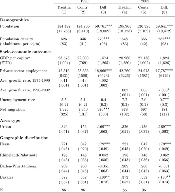
Table 2 presents summary statistics on several indicators for the treatment and control districts in our baseline sample for the years 1990 and 2002. Columns (1) and (4) report the means for the treatment districts and columns (2) and (5) report those for the control districts in 1990 and 2002 respectively. Columns (3) and (6) include the respective dierences and indicate the statistical signicance from t-tests on the equality of means. The treatment districts in our
27Specically, we rst ran a series of tobit regressions of log wages separately for each year, gender and education group with covariates that include a quartic in age and dummies for foreign citizenship, occupations, industries and the local districts (the results from theses estimations are available upon request). The top-coded wage observations were then replaced by draws from normal distributions that are truncated from below at the SSCT and the moments of which are determined from the respective tobit estimations. Büttner and Rässler (2008) and Büttner (2010) have recently criticized this homoscedastic single imputation as it may lead to biased variance estimates and develop a Bayesian multiple imputation method allowing for heteroscedasticity (MI-Het), which they can show to perform better in simulations with the IABS. Given the higher computational intensity of this approach and the fact that we use a much larger dataset with the entirety of records for a long panel, we decided to remain with the simpler method.
28As a single annual cross-section for all our districts consists of up to 8.4 million individual spells, working with the full population panel was not feasible due to standard limits of memory size and computational speed.
29While we do include these districts in our baseline sample, we conrm our results by excluding them in some of our later robustness checks, as these regions could potentially be inuenced by workers who commute to the other side of the border. Moreover, the districts that are located on the former border to East Germany or the Eastern border to other former member states of the Warsaw Pact benet from higher levels of regional subsidies (for example, from the European Regional Development Fund) in response to their marginal location.
sample have, on average, a higher population and are more densely populated. This is also reected in the gures of the third subpanel in Table 2: 33% of the treatment districts are located in urban areas compared with 16% of the control districts. The bottom panel quanties the geographic distribution across the four federal states (see Figure 5). It suggests that the spatial distribution is quite balanced, although within Hesse, the treatment districts outnumber the control districts. In the entire sample, this is compensated for by a higher share of control districts located in Bavaria.
In summary, the unconditional cross-sectional comparisons for the two selected years reveal some dierences between our treatment and control regions. The key identifying assumption in the dierence-in-dierence framework that we employ only requires that the outcomes in the treatment and control group follow similar time trends in the pre-treatment period (see Angrist and Krueger, 1999, Angrist and Pischke, 2009, chap. 5). Cross-sectional dierences only lead to a violation of this assumption if they aect changes in the outcomes in a time-varying way.
As outlined in the previous section, we control for any source of potential misspecication by including in all our regressions district and time-xed eects, and also estimate specications that are enriched by state-by-year xed eects and full sets of district-specic linear or quadratic time trends. Finally, given the strong variation in the U.S. force numbers at the district level, our identication relies as much on the comparison between the districts in the treatment group as on the comparison with districts in the control group.
5 Results
5.1 Employment
A. Initial Estimates
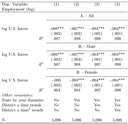
Table 3 reports the results for our initial OLS regression of equation (1). Each column presents three separate regressions of the log of total district private sector employment, with entries in panel A reporting the results for the pooled employment outcome of all employees and Panel B and C considering the outcome separately for male and female employment.
The regressions reported in the rst column include only the measure of the U.S. withdrawal treatment and district and year xed eects on the right hand side of the equation. The estimated
coecient is negative and statistically signicant, with the point estimate being larger for men than for women, and being more precisely measured for males. The second column adds state-by- year dummies for the four dierent federal states to the model in order to absorb state-specic shocks, with the estimate for the overall employment being virtually unaltered, although the point estimate for males drops slightly and that for females rises and is now signicant.
Once we add the full set of 130 district-specic linear time trends to the model in column (3), the precision of the estimates is increased considerably, with the size of the standard errors being more than halved. The absolute value of the negative coecient estimate drops to about 0.4 log points, but remains highly signicant. Replacing the linear by quadratic trends in column (4) only slightly alters the results, and the negative point estimate on the U.S. forces level variable remains highly signicant despite the inclusion of almost 550 covariates. The hypothesis that the state-year interactions or district-specic time trends are jointly zero is strongly rejected by the data in standard F-tests. In these two nal specications, the eects are the same both in magnitude and in terms of precision for the two genders.
The size of the coecients in the last two specications suggests that the elasticity of private sector employment with respect to the reduction of U.S. Forces is -.004. This implies that a reduction of U.S. forces by 100 persons leads to a loss of about 4.6 full-time private sector jobs.30 In the remainder of the paper, we always tabulate results for the latter two specications that include the district-specic linear or quadratic time trends and which provide in our view robust and conservative estimates of the withdrawal eect. 31
B. Heterogeneity of eects
As argued in the introduction, the U.S. withdrawal shock constituted a consumption shock that aected local labor demand because it was concentrated among locally produced, non-traded goods and services. In this section, we test this notion by allowing for heterogeneity of eects across dierent subsets of total district employment. We rst partition local employment along the industry margin.
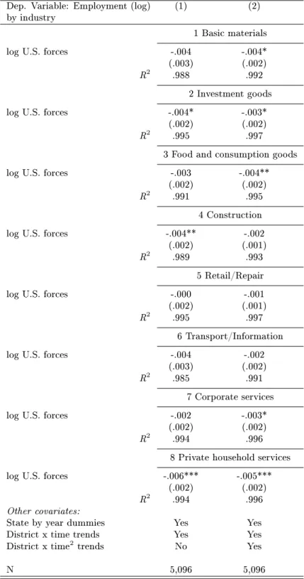
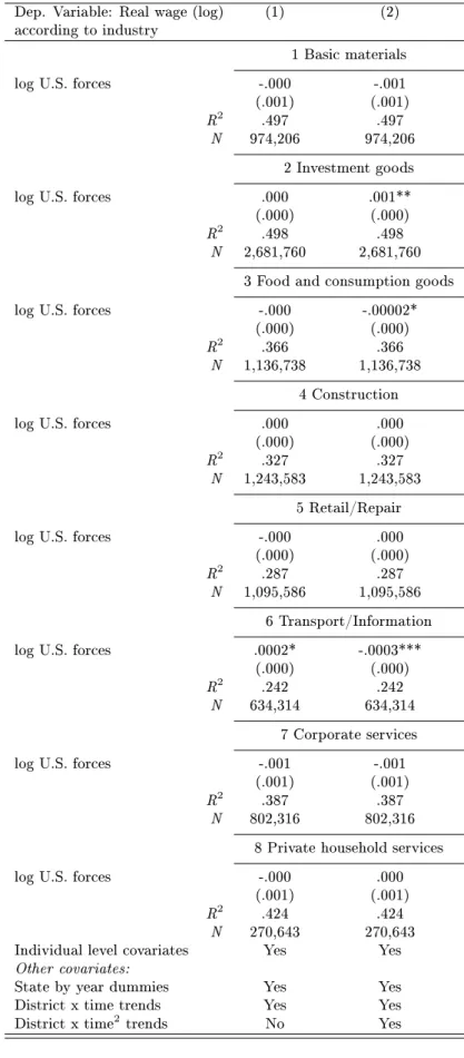
Table 4 shows the results for specications analogous to specication (1), estimated for
30The mean level of U.S. forces was about 3,700 in 1990, and the mean level of private sector employment in treatment regions was about 42,300.
31We have also tested specications that include a square or cubic function of our treatment variable, but these specications were rejected in favor of the simpler linear model.
employment separated according to industry groups.32 Consistent with the nature of the shock, the largest and most signicant eects are found in the sectors of food and consumption goods, and particularly private household services.
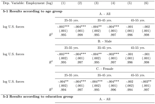
The top part of Table 5 provides estimates for our withdrawal coecient for the district employment in the three age groups (again subdivided in panels according to gender), with odd-numbered columns reporting the specications with linear, and even-numbered columns the specications with quadratic district time trends. The coecient estimates suggest that the adverse eect of the withdrawal mainly manifests itself in lower employment growth for younger male and female and for older female workers, while the point estimates for the other groups are smaller in absolute value and not signicantly dierent from zero. Similarly, the bottom part of the table reveals that it is primarily the employment of low and medium educated workers that is aected, although surprisingly, we nd the strongest eects of approximately -0.5 to -0.7 log points for the employment of high-qualied female workers.
C. Dynamic pattern of eects
In the analysis thus far, we have employed the traditional DD setting that presumes discrete changes in the treatment variable leading to instantaneous eects on the outcome of interest an assumption that is likely not to hold in our context: even if individual bases were closed down swiftly after the announcement was made, the force reductions at the district level in most cases took a couple of years to reach their full extent. The single coecient on the treatment variable would then fail to capture these longer-term eects. Similarly, although the rst base closure announcement for a district came as a surprise to the agents in the local economy, as we have argued in section 2.2, employers in districts that were only aected late in the withdrawal phase could still have responded by reducing their labor demand before the rst announcement for their district occurred if they expected cuts to reach their area at a later stage. These anticipatory eects could lead the estimates of the single coecient for the withdrawal treatment to be biased towards zero. Since the timing of the withdrawal, measured by the rst announcement in a district, exhibits some variation across treatment districts, we can identify and explore the dynamic pattern of the eect separately from the overall year
32We only tabulate the results here for the total employment (male and female) by industry since the estimates do not vary systematically by gender. The more detailed results from the separate estimations are available upon request.
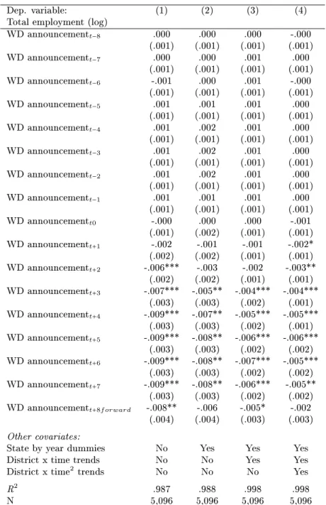
eects by augmenting the specication from equation (1) with lead and lag eects. We chose a symmetric window that includes eight lead variables for the eight years before the rst withdrawal announcement occurred and eight lag variables for the years 0-7 and year 8 onwards, as our selection of treatment and control districts allows us to have a balanced sample over this time span.
Table 6 presents the results when we reestimate the eect on total district employment in the augmented model using all four dierent specications again regarding the combination of state by year dummies and linear or quadratic time trends. In all four specications, the coecients on the withdrawal announcement leads are hardly signicantly dierent from zero, showing little evidence of anticipatory employment responses. More importantly, the point estimates on the withdrawal treatment delays continuously become more negative and signicant, starting from approximately -0.3 log points in year 2 after the withdrawal announcement up to -0.7 log points after ve to six years. Notably, the coecient for the long term eect for year 8 onwards still exhibits a negative eect that is at least in some specications signicantly dierent from zero.
This dynamic pattern is depicted for all four dierent specications in gure 6.
The diusion of the eect with stronger negative coecients several years after the with- drawal started in a district is in line with our expectation that the reduction in local demand is only incorporated and adjusted for with some time delay. However, the persistence of the negative steady state eect until at least 7 years after the start of the withdrawal might be surprising if one rather expects the eect to fade o at some time. Given our sample period, the results do not preclude that a mean reversion might occur in later periods, particularly, since we do not incorporate in our empirical approach information on the size and timing of redevelop- ment and conversion eorts in the treatment districts that could compensate for the reduction in employment from the withdrawal of the U.S. forces. However, the available case study literature suggests that apart from a small number of high-prole exceptions, the planning of local conver- sion projects took several years before they even started to be implemented.33 In addition, even if conversion projects were successful in promoting local economic development and employment growth, this would lead our estimates to underestimate the true negative eects, and not the other way around.
33See Cunningham and Klemmer (1995); Bonn International Center for Conversion (BICC) (1996). Brauer and Marlin (1992) also provide a general overview of the specic challenges of conversion in the economics literature.
D. Further Robustness Checks
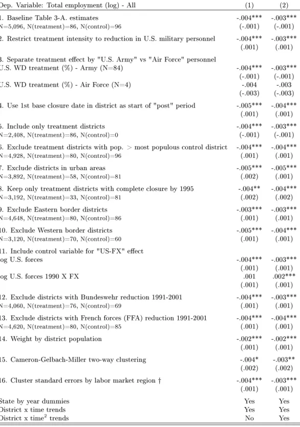
We close our empirical analysis on the employment eects by describing some alternative checks on the robustness of our results. While the augmented specication with lead and lag eects from the previous section is probably the most appropriate and exible one for ascertaining the local eects from the U.S. withdrawals, we return here for ease of exposition to the simpler specication from equation (1). Table 7 reproduces in row 1 the coecient estimates for the eect on total district employment from the top panel in column (7) and (8) of table 3 as a baseline for comparison.
We rst consider the robustness with respect to alternative denitions of our treatment variable. Row 2 reports the estimates for a specication in which the treatment intensity is not dened by the change in the total U.S. personnel level, but only by the change in the military positions. The idea is that the civil employees could potentially have stayed in the respective district and continued to consume in the local economy, living o income from alternative jobs or unemployment benets. The results are not aected by this change in the treatment variable.
The next specication examines whether the treatment eect diers for the withdrawal of U.S.
Army versus U.S. Air Force troops. Unfortunately, the Air Force withdrawals aect only 4 districts, so while the absolute value of the point estimates is comparable to the U.S. Army estimates, the Air Force coecient is no longer signicant given the larger standard errors.
Another variation of our baseline specication uses the rst actual base closure date instead of the rst announcement date as the identication of the start of the "post-treatment period".
Again, the coecient estimates are virtually unaltered.
Next, we consider the robustness with respect to alternative sample denitions. Row 5 reports results where we only use the variation in treatment intensity within the group of our treatment districts to identify the withdrawal eect. The point estimates remain almost identical to the baseline. Similarly, the exclusion from the sample of very populous treatment districts (given the structural dierences in the population size between treatment and control districts described in the summary statistics in section 4), of districts located in urban areas, of treatment districts that saw only a partial reduction of the U.S. force level, or of Eastern or Western border districts does not seem to aect the coecient estimates.
In the specications reported in Rows 11 to 13, we study the potential inuence of three
specic alternative district-specic shocks that could potentially bias our coecient estimates.
The results in row 11 stem from a specication in which we include an additional covariate (labeled U.S. Forces 1990 X FX) that interacts the log U.S. forces level in a given district in 1990 (before the start of the drawdown) with the average annual U.S. dollar to German DM exchange rate. This term is supposed to absorb the eects from the elasticity of the U.S.
demand active in the West German economy with respect to uctuations of the exchange rate that would have occurred even if the local force level had remained constant throughout our sample period.34 By introducing a covariate that explicitly captures this eect, we rule out any negative eects on the local economy that may have occurred already before and/or independent of any reductions in U.S. force levels, and thereby reinforce our identication assumption. The coecient estimate on this term is highly signicant (at least in the specication with quadratic time trends) and has the expected positive sign (i.e. a devaluation of the U.S. dollar seems to be associated with a drop in labor demand in the local economy). Reassuringly, our estimate of the U.S. forces coecient hardly diers from the baseline estimates.
During the time period of the U.S. withdrawal, the German Army and the French forces (Forces Françaises en Allemagne) also implemented realignments of their bases as part of the CFE treaty. Although smaller in absolute and relative size, these cuts more likely aected the control districts in our sample, due to the spatial partitioning of the combined military presence with the U.S. forces as NATO allies. Figure 8 depicts the regional presence by the German armed forces as a share of the district population in 1991 and identies the districts where realignments took place between 1991 and 2002, while Figure 9 depicts the districts within the four federal states that also hosted bases of the French forces.35 If we exclude these districts subsequently from the treatment and control groups, the estimates in row 12 and 13 reveal that the concurrent cuts by the German armed forces and the French forces do not seem to aect our estimates of the U.S. withdrawal eect signicantly.
As already summarized in our discussion of the empirical approach in section 3, the question
34Bebermeyer and Thimann (1990) note that the 50 percent decrease in the value of the US currency relative to the D-mark from 3.30 in March 1985 to 1.65 in January 1988 has meant a corresponding cut in the purchasing power of US servicemen stationed in the FRG. They document that this devaluation did not only lead to a reduction of the private American demand active in the local economy at the time, but also incited the U.S.
bases to reduce their number of German direct employees and substitute some goods previously sourced from West German suppliers with imports from U.S. companies. Figure 7 plots the time series of the exchange rate for our sample years 1975 to 2002.
35For details on the respective data sources, see section C.3 and C.4 in the Data Appendix.
of the correct calculation of standard errors and inference in DD settings has recently received increasing scrutiny. In our baseline estimates, we have always reported robust standard errors clustered on the district level that allow for arbitrary correlations within districts over time.
Row 14 of table 7 presents the results if we additionally weight the district-year observations by the district population in order to account for potential heteroscedasticity of the error term.
The coecient estimates are again only slightly reduced in their absolute value, and remain highly signicant. Next, we also used an alternative specication of the standard errors recently proposed by Cameron et al. (2011). Their method aims to improve inference in situations with non-nested multi-way clustering, and they specically mention the case of state-year panels where, in principle, it could be desirable to cluster both on the geographic unit (to allow for serial autocorrelation) and year level to account for geographic-based spatial correlation. In the case of two-way clustering, the estimator is calculated by adding up the variance matrices from OLS regressions with errors clustered on the rst and second dimension respectively, and then subtracting the variance matrix from a regression with errors clustered on both dimensions. We implement the estimator in our data, with the two dimensions being district and year. The estimated coecients reported in row 15 remain signicant at the 5 and 10 percent level despite the augmented standard errors. A further conservative alternative to account for potential spatial correlation that could bias standard errors downwards is to cluster at higher regional levels of aggregation. In this vein, Row 16 presents the coecient estimates once we cluster the errors on the levels of German labor market regions: reassuringly, the increase in the standard errors is minuscule, so that the results do not dier from the baseline in a meaningful way.36 5.2 Wages
In our analysis thus far, we have documented that the withdrawal of U.S. forces did indeed negatively aect employment in the German local labor markets where they were located. In light of this evidence, we now address the question of whether the withdrawal also led to a downward adjustment of local wages. As already described in sections 3 and 4, we base our wage analyses on random subsamples of the individual employment spells from male employees for each district and year in our sample period.
36We also repeated the whole empirical analysis at this higher aggregation level of labor market regions. The coecient estimates on the U.S. forces variable were negative and highly signicant in all specications, despite the lower variation in the treatment variable and the smaller number of observations.
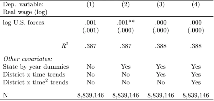
Tables 8 to 10 present the results from DD estimations of equation 2 of real gross daily wages (in logs), in breakdowns analogous to our employment analyses. All regressions include the full set of available individual-level covariates (age, age2, dummies for foreign citizenship, education levels, occupational groups) and the control variable for the exchange rate eect. The estimates for the overall wage eect in Table 8 and separately according to age and education groups in Table 9 are hardly signicantly dierent from zero and suggest that local real wages did not respond to the withdrawal shock. If anything, older and low qualied workers seem to enjoy some relative wage increases in the aected districts, an eect that might stem from the primary selection of younger workers to be dismissed. The analyses according to industries in Table 10 only reveal some evidence of potential downward wage adjustments for the sectors of "Food and consumption goods" and "Transport/Information".
5.3 Impact on Unemployment and Migration
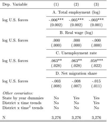
In this section, we use aggregate district-level data to examine the impact of the U.S. withdrawal shock on unemployment and migration and provide further evidence of the relative importance of the potential margins of adjustment in response to the withdrawal shock. The Statistics Department of the German Federal Employment Agency (Bundesagentur für Arbeit, BA) pub- lishes a time series on district level data on the number of unemployed and the unemployment rate starting in late 1984. Consistent with our timing convention for employment, we use the so-called quarterly statistic reported for the month of June in each year. To analyze the migra- tion response, we use aggregated data on net migration (the dierence in the number of in-ward migrants versus out-ward migrants) provided by the Statistische Ämter des Bundes und der Länder (2011) and from complimentary data requests with the individual state statistical oces to construct a consistent panel of district-year observations for the period 1985 to 2002.37
In table 11, we rst report in panel A and B the results for the estimated impact on total employment and wages for the comparable shorter time period from 1985-2002.38 The coecient estimates are consistent with our previous estimates for the longer time period from 1975-2002
37Unfortunately, more detailed migration data that reports the number of in-ward migrants and out-ward migrants separately and in further splits by age groups, gender and citizenship is only available at the district level from 1995 onwards.
38We focus here on the rst three specications with district and year FE only (1), the inclusion of state-by-year eects (2) and linear district-specic time trends (3), as our results indicate that we cannot robustly estimate the specication with quadratic district-specic trends in this shorter period in which the number of district observations in the pre-period before the withdrawal starts is more than halved compared to the period before.
(see tables 3 and 8), with signicant negative eects for local private sector employment and no adjustment in local wages. Panel C reports the coecient estimates for an analogous DD regression with the district unemployment rate as dependent variable. The results suggest that the withdrawal of the U.S. forces increased unemployment.Panel D provides results from the DD estimation on the net district migration share.39 The negative sign of the coecient estimates suggests a shift in the balance of migration towards greater out-ward migration in the treatment districts after the withdrawal, but none of the estimates is statistically signicant.
As argued previously for our employment outcome in section 5.1, the estimates for the year- by-year eect could mask a richer pattern of dynamic adjustments, particularly if unemployment and migration are only aected with some timedelay. In table 12, we hence present results from analogous regressions of the dynamic pattern for all outcomes for the time period 1985 to 2002.40 Column (1) reports the coecient estimates for the withdrawal leads and lags for employment.
Consistent with the previous results in table 6 for the "long" sample period, all lead coecients are statistically indistinguishable from zero, and the signicant negative coecient estimates on the withdrawal delays in the post period reach their peak around 5 years after the rst withdrawal announcement. For real wages in column (2), the results conrm the absence of any signicant adjustment eects throughout the whole observation period.
The dynamic pattern of the coecient estimates for the eect on unemployment and the unemployment rate in columns (3) and (4) does indeed provide some suggestive evidence that the decline in employment was (partially) absorbed by rising unemployment. Even if some lead eects are also marginally signicant, the pattern of the lagged eects provides a consistent picture of continuously larger coecient estimates up to a peak in years 5 to 6 after the initial withdrawal shock. The coecient estimates remain at this level even through the long term eect for year 8 onward, but the lower precision and loss of signicance for the estimates after year 7 prevent conclusive inference on the persistence of the rise in unemployment. Finally, column 5 shows the results for the comparable regressions for the net migration share. Again, the coecient estimates in the pre-withdrawal period are statistically indistinguishable from zero.
The estimates on the lag eects all have a negative sign and are larger in absolute value. However,
39We dene the net migration share by dividing the net migration balance in year t by the district population in year t-1.
40For compactness, we focus here on the specication that includes linear time trends and a consistent time period of between 5 years before and 8 or more years after the beginning of the withdrawal in a given district.
only the coecient estimate for year 3 after the withdrawal announcement is signicant at the 5 percent level. In light of the data limitations outlined above, we interpret this as a qualitative indication that some of the adjustment in response to the withdrawal shock could also occur via increased out-ward or reduced in-ward migration in the aected regions.
Overall, our comparison of the estimated adjustment eects suggest that the withdrawal shock primarily led to adjustments in quantities, and not in prices (i.e. wages). This nding is consistent with Topel's (1986) result for the eect from a permanent local economic shock.
6 Conclusion
Empirical research has had diculty in establishing the causal eects of local economic shock, and one important reason for this issue is that the measurement of local economic shocks has proven to be dicult. In this paper, we exploit the district variation in the stationing and withdrawal of U.S. military forces in Germany after German reunication and the end of the Cold War to examine the consequences of regional economic shocks on local labor market outcomes.
The unique natural experiment setting of the event allows us to improve on limitations that impaired previous studies analyzing the eect of regional economic shocks on local labor markets.
The U.S. forces were stationed in West Germany in the 1950 at strategic points along two major defense lines; local economic considerations were not important in this decision process. In addition, and in a similar fashion to the stationing decision, the withdrawal decisions for the U.S. forces in Germany were made exclusively by U.S. military ocials and were neither subject nor responsive to any politicizing: the U.S. Department of Defense decided on the details of the withdrawal process purely on strategic military grounds. Both of these facts alleviate concerns regarding the validity of exogeneity assumptions.
The results show that the withdrawal of the U.S. forces did have negative consequences for private sector employment and for local unemployment. Wages and migration patterns, however, were not aected.