Transient tracer distributions in the Fram Strait in 2012 and inferred anthropogenic carbon content and transport

(1)

www.ocean-sci.net/12/319/2016/

doi:10.5194/os-12-319-2016

Transient tracer distributions in the Fram Strait in 2012 and inferred anthropogenic carbon content and transport

Tim Stöven¹, Toste Tanhua¹, Mario Hoppema², and Wilken-Jon von Appen²

1Helmholtz Centre for Ocean Research Kiel, GEOMAR, Kiel, Germany

2Alfred Wegener Institute Helmholtz Centre for Polar and Marine Research, Bremerhaven, Germany

Correspondence to: Tim Stöven (tstoeven@geomar.de)

Received: 5 August 2015 – Published in Ocean Sci. Discuss.: 24 September 2015 Revised: 12 January 2016 – Accepted: 3 February 2016 – Published: 25 February 2016

Abstract. The storage of anthropogenic carbon in the ocean’s interior is an important process which modulates the increasing carbon dioxide concentrations in the atmosphere.

The polar regions are expected to be net sinks for anthropogenic carbon. Transport estimates of dissolved inorganic carbon and the anthropogenic offset can thus provide information about the magnitude of the corresponding storage processes.

Here we present a transient tracer, dissolved inorganic carbon (DIC) and total alkalinity (TA) data set along 78^◦50⁰N sampled in the Fram Strait in 2012. A theory on tracer relationships is introduced, which allows for an application of the inverse-Gaussian–transit-time distribution (IG-TTD) at high latitudes and the estimation of anthropogenic carbon concentrations. Mean current velocity measurements along the same section from 2002–2010 were used to estimate the net flux of DIC and anthropogenic carbon by the boundary currents above 840 m through the Fram Strait.

The new theory explains the differences between the theoretical (IG-TTD-based) tracer age relationship and the specific tracer age relationship of the field data, by saturation effects during water mass formation and/or the deliberate release experiment of SF6 in the Greenland Sea in 1996, rather than by different mixing or ventilation processes. Based on this assumption, a maximum SF6 excess of 0.5–0.8 fmol kg⁻¹ was determined in the Fram Strait at intermediate depths (500–1600 m). The anthropogenic carbon concentrations are 50–55 µmol kg⁻¹in the Atlantic Wa- ter/Recirculating Atlantic Water, 40–45 µmol kg⁻¹ in the Polar Surface Water/warm Polar Surface Water and between 10 and 35 µmol kg⁻¹in the deeper water layers, with lowest concentrations in the bottom layer. The net fluxes

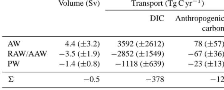
through the Fram Strait indicate a net outflow of∼0.4 DIC and∼0.01 PgC yr⁻¹anthropogenic carbon from the Arctic Ocean into the North Atlantic, albeit with high uncertainties.

1 Introduction

Changes in the Arctic during the last decades stand in mu- tual relationship with changes in the adjacent ocean areas such as the Nordic Seas, the Atlantic and the Pacific oceans.

The temperature of the Atlantic Water flowing into the Arc- tic Ocean through the Fram Strait has warmed since 1997 (Beszczynska-Möller et al., 2012), which thus increased the heat flux into the Arctic. This has a significant influence on the perennial sea ice thickness and volume and thus on the fresh water budget (Polyakov et al., 2005; Stroeve et al., 2008; Kwok et al., 2009; Kurtz et al., 2011). The exchange and transport of heat, salt and fresh water through the major gateways like the Fram Strait, Barents Sea Opening, Canadian Archipelago and Bering Strait are also directly related to changes in ventilation of the adjacent ocean areas (Wadley and Bigg, 2002; Vellinga et al., 2008; Rudels et al., 2012). The ventilation processes of the Arctic Ocean have a significant impact on the anthropogenic carbon storage in the world ocean (Tanhua et al., 2008). Studying the fluxes of anthropogenic carbon through the major gateways contributes to understand the integrated magnitude of such ocean-atmosphere interactions. It additionally provides information of a changing environment in the Arctic Mediter- ranean. The required flux data of the prevailing water masses, i.e., current velocity fields, are obtained by time series of long-term maintained mooring arrays in the different gate-

(2)

ways. The Fram Strait is the deepest gateway to the Arc- tic Ocean with highest volume fluxes equatorward and pole- ward. A well-established cross-section mooring array is located at∼78^◦50⁰N in the Fram Strait (Fahrbach et al., 2001;

Schauer et al., 2008) and has provided the basis for heat transport estimates in the past (Fahrbach et al., 2001; Schauer et al., 2004, 2008; Beszczynska-Möller et al., 2012). How- ever, the current data interpretation and analysis of this mooring array is complicated due to a recirculation pattern in the Fram Strait (Schauer and Beszczynska-Möller, 2009; Rudels et al., 2008; Marnela et al., 2013; de Steur et al., 2014) and strong mesoscale eddy activity (von Appen et al., 2015a).

The spatial and temporal volume flux variability and the insufficient instrument coverage in the deeper water layers, i.e., below the West Spitsbergen Current (WSC) and East Green- land Current (EGC), lead to high uncertainties of the net flux through the Fram Strait. Hence, it is the most relevant but also the most challenging gateway with respect to transport budgets in the Arctic Mediterranean.

Estimating an anthropogenic carbon budget presupposes the knowledge of the concentration ratio between the nat- ural dissolved inorganic carbon (DIC) and anthropogenic carbon (C_ant) in the water column. An estimate of DIC transport across the Arctic Ocean boundaries is provided by MacGilchrist et al. (2014), who used velocity fields by Tsub- ouchi et al. (2012) and available DIC data. That work provides a proper estimate of DIC fluxes, although it does not separate the specific share of anthropogenic carbon and the uncertainties are relatively high. Similarly, Jeansson et al.

(2011) calculated fluxes of inorganic, organic and anthropogenic carbon to the Nordic Seas using an extensive set of carbon and transient tracer data. Here we present anthropogenic carbon column inventories in the Fram Strait using a new data set of SF₆ and CFC-12 along the cross-section of the mooring array at 78^◦50⁰N. The anthropogenic carbon column inventories were estimated using the transient tracers and the inverse-Gaussian–transit-time distribution (IG-TTD) model. Flux estimates of DIC and anthropogenic carbon including the Atlantic Water, Recirculating Atlantic Water, Arctic Atlantic Water and Polar Water water masses through the Fram Strait above 840 m are provided based on mean velocities measured with moorings between 2002 and 2010.

Common error sources and specific aspects using these tracers and this method in the Fram Strait are highlighted.

2 Material and Methods 2.1 Tracer and carbon data

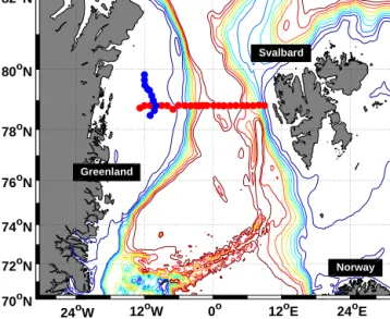
A data set of CFC-12, SF₆, DIC and TA was obtained during the ARK-XXVII/1 expedition from 14 June to 15 July 2012 from Bremerhaven, Germany to Longyearbyen, Svalbard on the German R/V Polarstern (Beszczynska-Möller, 2013).

Figure 1 shows the stations of the zonal section along

12ôW 0ô 12ôE 24ôE 70ôN

72ôN 74ôN 76ôN 78ôN 80ôN 82ôN

24^oW

Svalbard

Greenland

Norway

Figure 1. Sample stations of the ARK-XXVII/1 cruise in 2012. The zonal stations are highlighted as red dots and the meridional stations along the fast ice edge as blue dots. The depth contours are 250: 250:2500.

78^◦50⁰N, where measurements of CFC-12, SF₆, DIC and TA were conducted. The meridional section along the fast ice edge was only sampled for CFC-12 and SF6and shows no differences in the horizontal tracer distributions compared to the corresponding longitude range of the zonal section.

Therefore, we have only used the zonal section for the following analysis.

Water samples for the determination of the transient tracers CFC-12 and SF₆were taken with 250 mL glass syringes and directly measured on board, using a purge and trap GC-ECD system similar to Law et al. (1994) and Bullister and Wisegarver (2008). The measurement system is iden- tical to the PT3 system described in Stöven and Tanhua (2014) except for the cooling system and column compo- sition. The trap consisted of a 1/16⁰⁰ column, packed with 70 cm HayeSep D and cooled to−70^◦C during the purge process using a Dewar filled with a thin layer of liquid ni- trogen. The 1/8⁰⁰ precolumn was packed with 30 cm Porasil C and 60 cm Molsieve 5A and the 1/8⁰⁰ main column with 180 cm Carbograph 1AC. Due to malfunctioning of the Elec- tron Capture Detector (ECD) of the measurement system, the samples of six stations (between station 15 and 53) were taken with 300 mL glass ampules and flame sealed for later onshore measurements at GEOMAR. The onshore measurement procedure is described in Stöven and Tanhua (2014).

The precision for the onshore measurements is±4.4 %/0.09 for SF₆and±1.9 %/0.09 pmol kg⁻¹for CFC-12. The precision for onboard measurements is±0.5 %/0.02 for SF₆and

±0.6 %/0.02 pmol kg⁻¹for CFC-12.

Water samples for DIC and total alkalinity (TA) were taken with 500 mL glass bottles and poisoned with 100 µL of a saturated mercuric chloride solution to prevent bio-

(3)

logical activities during storage time. The sampling procedure was carried out according to Dickson et al. (2007).

The measurements of DIC and TA were performed onshore at the GEOMAR, using a coulometric measurement system (SOMMA) for DIC (Johnson et al., 1993, 1998) and a potentiometric titration (VINDTA) for TA (Mintrop et al., 2000). The precision is ±0.05 %/1.1 for DIC and

±0.08 %/1.7 µmol kg⁻¹ for TA. The data of all obtained chemical parameters are available at the Carbon Diox- ide Information Analysis Center (CDIAC; http://cdiac.ornl.

gov/oceans/RepeatSections/clivar_75N.html). The physical oceanographic data (temperature, salinity and pressure) from this cruise can be found in Beszczynska-Möller and Wisotzki (2012).

2.2 Water transport data

An array of moorings across the deep Fram Strait from 9^◦E to 7^◦W has been maintained since 1997 by the Al- fred Wegener Institute and the Norwegian Polar Institute.

Since 2002, it has contained 17 moorings at 78^◦50⁰N. Here we use the gridded data from the array from summer 2002 to summer 2010, as described in Beszczynska-Möller et al.

(2012). The more recent data have either not been recov- ered yet or the processing is still in progress. The moorings contained temperature and velocity sensors at five standard depths: 75, 250, 750, 1500 and 10 m above the bottom. The hourly measurements were averaged to monthly values and then gridded onto a regular 5 m vertical by 1000 m horizontal grid using optimal interpolation. While the Atlantic Water in the Fram Strait has warmed since 1997, Beszczynska-Möller et al. (2012) showed that there is a strong seasonal cycle in the Atlantic Water transport through the Fram Strait, but that there is no statistically significant interannual trend between 1997 and 2010 in the volume transport. We consider the long- term average volume flux of the following water masses:

Atlantic Water advected in the WSC, defined as longitude

≥5^◦E and depth ≤840 m; Polar Water flowing southward in the EGC, defined as mean temperature≤1^◦C and depth

≤400 m; and Recirculating and Arctic Atlantic Water which is both due to the recirculation of Atlantic Water in the Fram Strait (de Steur et al., 2014) and the long loop of Atlantic Water through the Arctic Ocean (Karcher et al., 2012), defined as longitude≤1^◦E and depth≤840 m, and not as Po- lar Water. The estimate of the volume transport across the Fram Strait below 840 m from the moorings is more complicated. The method of Beszczynska-Möller et al. (2012) which was developed to study the fluxes in the WSC pre- dicts a net southward transport of 3.2 Sv below 840 m. This is unrealistic, given that there are no connections between the Nordic Seas and the Arctic Ocean below the sill depth of the Greenland–Scotland Ridge (840 m) other than the Fram Strait. No vertical displacements of isopycnals in these two basins are observed that would suggest a non-zero net transport across the Fram Strait below 840 m (von Appen et al.,

2015b). The large net transport inferred by Beszczynska- Möller et al. (2012) is due to the insufficient horizontal reso- lution of the mooring array to explicitly resolve the westward flow of the recirculation and the mesoscale eddies. For these reasons, we assume a net flux of 0 Sv across the Fram Strait for the deep waters below 840 m.

2.3 TTD method

A transit time distribution (TTD) model (Eq. 1) describes the propagation of a boundary condition into the interior of the ocean and is based on Green’s function (Hall and Plumb, 1994).

c(t_s, r)=

∞

Z

0

c₀(t_s−t )e^−λt·G(t, r)dt (1)

Here,c(t_s, r)is the specific tracer concentration at yeart_sand locationr,c₀(t_s−t )the boundary condition described by the tracer concentration at source yeart_s−t, andG(t )the transit time distribution of the tracer. The exponential term cor- rects for the decay rate of radioactive transient tracers. Equa- tion (2) provides a possible solution of the TTD model, based on a steady and one-dimensional advective velocity and dif- fusion gradient (Waugh et al., 2003).

G(t )= s

0³ 4π 1²t³·exp

−0(t−0)² 41²t

(2)

It is known as the inverse-Gaussian–transit-time distribution (IG-TTD) whereG(t )is defined by the width of the distribution (1), the mean age (0) and the time range (t). One can define a1/ 0ratio of the IG-TTD which represents the proportion between the advective and diffusive properties of the mixing processes as included in the TTD. The lower the 1/ 0ratio, the higher is the advective share. A1/ 0 ratio of 1.0 is the commonly applied ratio (unity ratio) at several tracer surveys (e.g., Waugh et al., 2004, 2006; Tanhua et al., 2008; Schneider et al., 2010, 2014; Huhn et al., 2013).

Another approach is based on a linear combination of two IG-TTDs which can be used to describe more complex ventilation patterns (Eq. 3) (Waugh et al., 2002). The variables of this model are 11,2 and01,2 of the two IG-TTDs and α, which describes the ratio between both distributions. The main problem of applying this method is that five free parameters need to be determined. Hence, this model combination can be constrained with five transient tracers with sufficiently different input functions. Alternatively, predefined parameters can be used (Stöven and Tanhua, 2014).

c(ts, r)=

∞

Z

0

c0(ts−t )e^−λt·

[α G(0₁, 1₁, t, r)+(1−α) G(0₂, 1₂, t, r)] dt (3)

(4)

Note that the use of CFC-12 as transient tracer is limited to concentrations below the recent atmospheric level since the production of CFC-12 was phased out in the early 1990s so that the depletion rate exceeds the emission rate from the early 2000s on. This causes indistinct time information of CFC-12, since one concentration describes two dates in the atmospheric history. To this end, the use of CFC-12 is restricted to water masses with concentrations below the current atmospheric concentration limit. The emission rate of SF₆still exceeds the depletion rate so the atmospheric concentration still increases. SF6thus provides distinct age information of water masses over the complete concentration range.

2.4 Anthropogenic carbon and transport estimates The IG-TTD model can be used to estimate the total amount of anthropogenic carbon in the water column (Waugh et al., 2004). For this purpose it is assumed that the anthropogenic carbon behaves like an inert passive tracer, i.e., similar to a transient tracer. By applying Eq. (1), the concentration of anthropogenic carbon in the interior ocean (Cant(ts)) is given by Eq. (4).

C_ant(t_s)=

0

Z

∞

C_ant,0(t_s−t )·G(r, t )dt (4)

Cant,0 is the boundary condition of anthropogenic carbon at yearts−t andG(r, t )the distribution function (see Eq. 1).

The historic boundary conditions are described by the differences between the preindustrial and modern DIC concentrations at the ocean surface. These anthropogenic offsets can be calculated by applying the modern (elevated) partial pressures of CO₂and then subtracting the corresponding value of the preindustrial partial pressure. In each case, the preformed alkalinity was used as second parameter to determine the specific DIC concentrations (calculated using the Matlab ver- sion of the CO2SYS, van Heuven et al., 2011). Here we assumed a constantpCO_2,watersaturation in the surface. Since exact saturations are not well constrained, we present sensi- tivity calculations of different saturation states/disequilibria (see Sect. 3.6 below). The atmospheric history ofpCO2,atmis taken from Tans and Keeling (2015). The preformed alkalinity was determined by using the alkalinity–salinity relationship of MacGilchrist et al. (2014). This relationship is based on surface alkalinity and salinity measurements in the Fram Strait which were corrected for sea-ice melt and formation processes.

The time-dependent boundary conditions (C_ant,0) and Eq. (4) can then be used to calculate anthropogenic carbon concentrations (C_ant(t_s)) and the corresponding mean age.

Finally, the mean age of Eq. (4) can be set in relation to the transient tracer-based mean age of the water and allows for back-calculating C_ant(t_s), i.e., it provides the link between

the tracer concentration and the anthropogenic carbon concentration.

We then proceed to estimate transports of anthropogenic carbon through the Fram Strait. Transports are the product of concentrations multiplied by velocities integrated over an area. We assume that the trace gas concentrations change relatively slowly between years and that there are no significant seasonal changes. Hence, we can take the concentrations from summer 2012 to be informative about other seasons and years within some range from 2012. On the other hand, it is known that velocities change strongly between seasons (and on shorter time scales), but on average not sig- nificantly between years in the Fram Strait (Beszczynska- Möller et al., 2012). It follows that the measured (2002–

2010) long-term average volume transport is representative of the volume transport through the Fram Strait in the late 2000s–early 2010s. Likewise, the measured C_antconcentra- tions in summer 2012 are representative of the C_antconcen- trations in the late 2000s–early 2010s. The product of the two is then our estimate of the C_anttransport through the Fram Strait in the late 2000s–early 2010s.

3 Results and Discussion

3.1 Water masses in the Fram Strait

To highlight the different transient tracer characteristics, we defined the water mass type of each sample by using the water mass properties suggested by Rudels et al. (2000, 2005) and the salinity and temperature data of this cruise from Beszczynska-Möller and Wisotzki (2012).

Water masses of the Arctic Ocean are the Polar Surface Water (PSW), which is the cold and low saline surface and halocline water; the warm Polar Surface Water, defined by a potential temperature (2)>0, which comprises sea ice melt water due to interaction with warm Atlantic Water and due to solar radiation; the Arctic Atlantic Water which derives from sinking Atlantic Water due to cooling in the Arctic Ocean. The deep water masses are upper Polar Deep Water (uPDW), Canadian Basin Deep Water (CBDW) and Eurasian Basin Deep Water (EBDW). Deep water formation, e.g., on the Arctic shelves, usually involves densification due to brine rejection. The Eurasian Basin Deep Water mixes with Green- land Sea Deep Water so that this layer corresponds to two sources in the Fram Strait (von Appen et al., 2015b).

Water masses of the Atlantic Ocean/Nordic Seas are the warm and saline Atlantic Water (AW) and the corresponding Recirculating Atlantic Water (RAW); the Arctic Intermedi- ate Water (AIW) which is mainly formed in the Greenland Sea; the Nordic Seas Deep Water (NDW) which comprises Greenland Sea Deep Water (GSDW), Iceland Sea Deep Wa- ter (ISDW) and Norwegian Sea Deep Water (NSDW) and is formed by deep convection during winter time.

(5)

PSW PSWw PDW AAW AIW CBDW EBDW/GSDW AW/RAW NDW

−12 −10 −8 −6 −4 −2 0 2 4 6 8 0

500 1000 1500 2000 2500

Longitude [°E]

Pressure [dbar]

Figure 2. Water masses in the Fram Strait: Nordic Seas Deep Water (NDW), Atlantic Water/Recirculating Atlantic Water (AW/RAW), Eurasian Basin Deep Water (EBDW)/Greenland Sea Deep Water (GSDW), Canadian Basin Deep Water (CBDW), Arctic Intermedi- ate Water (AIW), Arctic Atlantic Water (AAW), Upper Polar Deep Water (uPDW), Polar Surface Water warm (PSWw) and Polar Sur- face Water (PSW).

Figure 2 shows the zonal water mass distribution in the Fram Strait based on salinity and temperature data from the CTD. The surface layer is dominated by Atlantic Water and Recirculating Atlantic Water in the east and by Polar Sur- face Water in the west with a transition between 6^◦W and 4^◦E where Polar Surface Water overlays the Atlantic Wa- ter. Warm Polar Surface Water can be found within the At- lantic Water between 4 and 8^◦E. The Atlantic Water layer extends down to∼600 m. Arctic Atlantic Water can be found at the upper continental slope of Greenland between 300 and 700 m. The intermediate layer between 500 and 1600 m consists mainly of Arctic Intermediate Water and, at the Green- land slope, partly of Upper Polar Deep Water. Canadian Basin Deep Water can be found between 1600 and 2400 m west of 4^◦E. Nordic Seas Deep Water is the prevailing water mass along the continental slope of Svalbard between 700 and 2400 m but can be also observed in the range of the Cana- dian Basin Deep Water layer. The Eurasian Basin Deep Wa- ter/Greenland Sea Deep Water forms the bottom layer below 2400 m.

3.2 Transient tracer and DIC distributions

Figure 3 shows the partial pressure of CFC-12 and SF₆ at the zonal section across the Fram Strait. Both tracers have significant concentrations through the entire water column and show a similar distribution pattern. The Atlantic Water shows a relatively homogeneous distribution of both tracers, with CFC-12 partial pressures >450 ppt and SF6>6 ppt.

The Polar Surface Water at the shelf region shows a more distinct structure with partial pressures between 4 and 8 of SF₆and 410–560 ppt of CFC-12. The smaller concentration gradient of CFC-12 in the surface compared to SF₆ is related to the recently decreasing atmospheric concentration of CFC-12, which causes only slightly varying boundary conditions at the air–sea interface (see Sect. 2.3). The high-tracer- concentration layer of the Polar Surface Water extends further eastward as overlaying tongue of the Atlantic Water between 2 and 6^◦W. The intermediate layer between 500 and

−12 −10 −8 −6 −4 −2 0 2 4 6 8

0 500 1000 1500 2000

2500 50

50

100 100

150 150

200

250 250

250 300

300

350

400

400 400

400 450

450 450

500 500 50

0 500500

550 114 114 114 114 114 114 114 114 114 114

114112112112112112112112112112112112 115115115115115115115115115115115115115106106106106106106106106106106117117117117117117117117117117117117117 119119119119119119119119119119119 121121121121121121121121121121121 123123123123123123123123123123123123 125125125125125125125125125125 128128128128128128128128128128128128128128 132132132132132132132132132132132132132132132132132 135135135135135135135135135135135135135135135135135135135135 79 79 79 79 79 79 79 79 79 79 79 79 79 79 79 79 79 81 81 81 81 81 81 81 81 81 81 81 81 81 76 76 76 76 76 76 76 76 76 76 76 76 76 76 76 76 72 72 72 72 72 72 72 72 72 72 72 72 72 69 69 69 69 69 69 69 69 69 69 69 69 69 69 67 67 67 67 67 67 67 67 67 67 67 67 67 67 57 57 57 57 57 57 57 57 57 57 57 57 57 57 53 53 53 53 53 53 53 53 51 51 51 51 51 51 51 37 37 37 37 37 37 37 27 27 27 27 27 27 27 20 20 20 20 20 20 15 15 15 15 15

Longitude [°E]

Pressure [dbar] CFC−12 [ppt]

0 100 200 300 400 500 600

(a)

−12 −10 −8 −6 −4 −2 0 2 4 6 8

0 500 1000 1500 2000 2500

1 1

2

2 2

3

4

4 4

4 5

5 5

5 6

6 6

7

7 7 7 114

114 114 114 114 114 114 114 114 114

114112112112112112112112112112112112 115115115115115115115115115115115115115106106106106106106106106106106117117117117117117117117117117117117117 119119119119119119119119119119119 121121121121121121121121121121121 123123123123123123123123123123123123 125125125125125125125125125125 128128128128128128128128128128128128128128 132132132132132132132132132132132132132132132132132 135135135135135135135135135135135135135135135135135135135135 79 79 79 79 79 79 79 79 79 79 79 79 79 79 79 79 79 81 81 81 81 81 81 81 81 81 81 81 81 81 76 76 76 76 76 76 76 76 76 76 76 76 76 76 76 76 72 72 72 72 72 72 72 72 72 72 72 72 72 69 69 69 69 69 69 69 69 69 69 69 69 69 69 67 67 67 67 67 67 67 67 67 67 67 67 67 67 57 57 57 57 57 57 57 57 57 57 57 57 57 57 53 53 53 53 53 53 53 53 51 51 51 51 51 51 51 37 37 37 37 37 37 37 27 27 27 27 27 27 27 20 20 20 20 20 20 15 15 15 15 15

Longitude [°E]

Pressure [dbar] SF6 [ppt]

0 1 2 3 4 5 6 7 8

(b)

Figure 1

Figure 3. Distribution of the partial pressure of (a) CFC-12 and (b) SF₆along the zonal section in the Fram Strait.

1600 m is characterized by a clear tracer minimum along the continental slope of Greenland with partial pressures between 1.8 and 4.0 of SF6 and 150–350 ppt of CFC-12 and mainly comprises Arctic Atlantic Water. East of this minimum, a remarkable tracer maximum can be observed at 1–

3^◦W with partial pressures between 3 and 6 of SF6and 250–

450 ppt of CFC-12. A smaller maximum can be observed between 5 and 6^◦E at ∼1000 m with partial pressures of

∼5 of SF₆and∼330 ppt of CFC-12. Both tracer maxima likely correspond to recently ventilated water which mainly affected the Arctic Intermediate Water and partly the At- lantic Water in the transition zone of both water masses. The Arctic Intermediate Water in the Fram Strait thus consists of recently ventilated areas and less ventilated areas, which is also indicated by the large range of transient tracer concentrations. The remaining intermediate layer above 1700 m is characterized by lower partial pressures between 2 and 3 of SF6and 150–300 ppt of CFC-12 with concentrations decreasing with depth. This gradient extends throughout the deep water layers down to the bottom with partial pressures from 2 down to 0.2 ppt of SF6and from 150 down to 34 ppt of CFC-12.

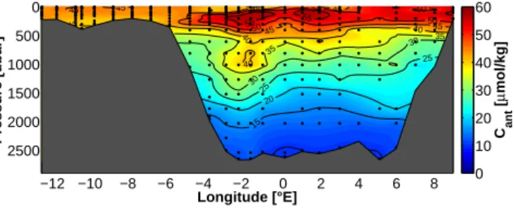
Figure 4 shows the DIC concentrations along the zonal section. The Greenland shelf region shows concentrations between 1970 in the surface and 2145 µmol kg⁻¹at∼200 m.

The upper 200 m between 4 and 8^◦E shows increasing concentrations with depth between 2070 and 2155 µmol kg⁻¹. There are three significant DIC maxima below 200 m. Two are located at the continental slope of Svalbard at 300–

800 and at 1400–2100 m, with concentrations>2158 and a maximum concentration of 2167 µmol kg⁻¹. The third max-

(6)

0 100 200

202520502075 2075

2100

2100 2125

2125 2125

2150 2150

114 114 114 114 114 114 114 114 114 114

114112112112112112112112112112112 115115115115115115115115115115115115115115 117117117117117117117117117117117117117117 119119119119119119119119119119119119 121121121121121121121121121121121 123123123123123123123123123123123123 125125125125125125125125125 128128128128128128128128128128128128 132132132132132132132132132132132132132132132132132132132 135135135135135135135135135135135135135135135135135135135135 79 79 79 79 79 79 79 79 79 79 79 79 79 79 79 79 79 81 81 81 81 81 81 81 81 81 81 81 81 81 81 81 81 76 76 76 76 76 76 76 76 76 76 76 76 76 76 72 72 72 72 72 72 72 72 72 72 72 72 72 72 72 69 69 69 69 69 69 69 69 69 69 67 67 67 67 67 67 67 67 67 67 67 67 57 57 57 57 57 57 57 57 57 57 57 57 57 53 53 53 53 53 53 53 53 53 53 53 53 51 51 51 51 51 51 51 51 51 51 51 51 51 51 37 37 37 37 37 37 37 37 37 37 37 27 27 27 27 27 27 27 27 27 27 20 20 20 20 15 15 15 15

1990 2080 2170

−12 −10 −8 −6 −4 −2 0 2 4 6 8

200 500 1000 1500 2000 2500

2150 2150

215

2152 2152

2152

2152 2152

2154

154

2154

21542156 2156 2156

2156 2156

2158 2158

2158

2160 2160 2160

2160

2162

2162 2164

Pressure [dbar]

Longitude [°E]

DIC [μmol/kg]

2140 2145 2150 2155 2160 2165

Figure 4. Distribution of dissolved inorganic carbon (DIC, in µmol kg⁻¹) along the zonal section in the Fram Strait.

imum corresponds to the transient tracer maximum at 1–

3^◦W but extends further eastward, with concentrations between 2158 and 2162 µmol kg⁻¹. The area of the EGC at 3–

8^◦W is characterized by concentrations between 2118 and 2152 µmol kg⁻¹. The deep water below 1700 m shows concentrations between 2150 and 2158 µmol kg⁻¹.

3.3 Transient tracers and the IG-TTD

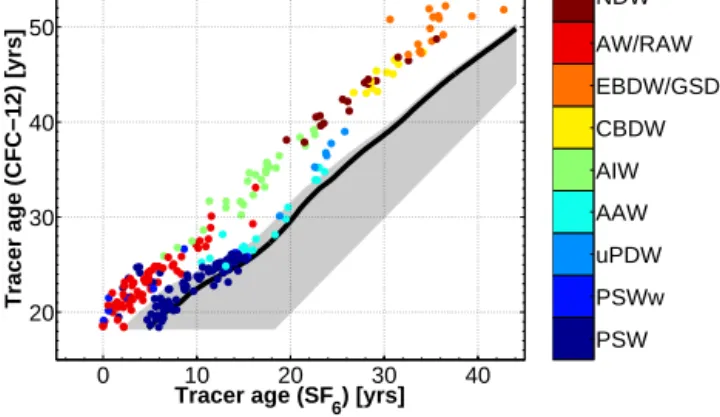
The IG-TTD can be numerically constrained using transient tracer couples, CFC-12 and SF6in our case, which provide information about the mean age and the parameters of the IG-TTD (Waugh et al., 2002; Sonnerup et al., 2013; Stöven and Tanhua, 2014). The method of validity areas, introduced in Stöven et al. (2015), is used to determine the applicability of the tracer couple. For this purpose, the tracer age is calculated from the transient tracer concentrations (Waugh et al., 2003) which provide the tracer age relationship of the tracer couple. Figure 5 shows the tracer age relationship of our field data (colored by water mass) in relation to the range of theoretical tracer age relationships of the IG-TTD, i.e., for1/ 0 ratios between 0.1 and 1.8, which describe the range from ad- vectively dominated to diffusively dominated water masses (grey shaded area). The black line in Fig. 5 denotes the tracer age relationship based on the unity ratio of1/ 0=1.0. Field data which correspond to this unity ratio would be centered around the black line.

The Fram Strait data can generally be separated into two sets of tracer age relationships. The upper set consists of water masses of Atlantic origin and deep waters, namely At- lantic Water/Recirculating Atlantic Water, Arctic Intermedi- ate Water, Nordic Seas Deep Water, Eurasian Basin Deep Water/Greenland Sea Deep Water and Canadian Basin Deep Water whereas the lower set only consists of water masses of polar origin, namely Polar Surface Water, warm Polar Sur- face Water, Arctic Atlantic Water and upper Polar Deep Wa- ter. Note that the Arctic Atlantic Water and upper Polar Deep Water merge with the upper set for SF₆tracer age larger than about 25 years. However, the upper set does not correspond to the unity ratio and, moreover, it is outside the validity area

PSW PSWw uPDW AAW AIW CBDW EBDW/GSDW AW/RAW NDW

Tracer age (CFC−12) [yrs]

Tracer age (SF

6) [yrs]

0 10 20 30 40

20 30 40 50

Figure 5. Validity area of the IG-TTD, defined by the tracer couple CFC-12 and SF₆(grey shaded area). The black line indicates the IG- TTD-based tracer age relationship using the unity ratio of1/ 0= 1.0. The field data are colored by the type of water mass. The lower set (blue dots) describes surface and intermediate water of Arctic origin whereas the upper set includes water of Atlantic origin and deep water masses.

of the IG-TTD. Water masses related to the lower set can be applied to the IG-TTD with tendencies toward higher1/ 0 ratios (>1.0) since the data are clearly above the black line, indicating a dominance of diffusive processes.

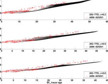
Another approach is provided by the linear combination of two IG-TTDs. Since we only have the data of two transient tracers, we used the same predefined parameters as described in Stöven and Tanhua (2014) which include one more diffusive water parcel (1₁/01=1.4) and one very advective water parcel (1₂/02=0.6). Similar to Figure 5,Fig. 6 shows the validity area of the linear combination of two IG-TTDs for differentαof 0.2, 0.5 and 0.8. Although this combination describes several scenarios from highly advective to diffusive mixing of two distributions, it can be seen that most of the observed data points are still outside the validity area. Thus, the tracer age relationship between CFC-12 and SF₆can be described neither by the IG-TTD nor a linear combination of two IG-TTDs.

Based on the raw field data and assumptions implemented in the IG-TTD (such as constant mixing processes along the flow pathway as well as constant saturation of the gases at the surface before entering deeper layers), the IG-TTD or linear combinations of the IG-TTD can only partly describe the ventilation pattern of water masses in the Fram Strait. Nev- ertheless, by comparing the shape of the two field data sets with the shape of the black line in Fig. 5, both sets show similar characteristics, such as the unity ratio or, generally, IG-TTD-based tracer age relationships. This opens up the possibility to use the IG-TTD the other way around, i.e., to assume a fixed1/ 0ratio to determine the deviation of transient tracer concentrations rather than using the transient tracer concentration to determine the1/ 0ratio. Since several publications found the unity ratio of1/ 0=1.0 to be

(7)

Figure 6. Validity areas of linear combinations of two IG-TTDs forα=0.2, 0.5, 0.8,1₁/0₁=1.4,1₂/0₂=0.6 and0_1,2=1–500 (black dots). The field data are described by the red crosses. The lower theαvalue, the higher the share of the diffusively dominated IG-TTD.

valid in large parts of the ocean, we assumed that this is also true for water masses in the Fram Strait. Figure 7 shows the mean tracer age relationship of the upper set (red line) and the tracer age relationship of the unity ratio (black line/same as in Fig. 5). The offset of the field data related to the unity ratio suggests an undersaturation of CFC-12 and/or a supersaturation of SF₆(see black box in Fig. 7). This uncommon coexistence of under- and supersaturated transient tracers is discussed in the following section.

3.4 Saturations and excess SF₆

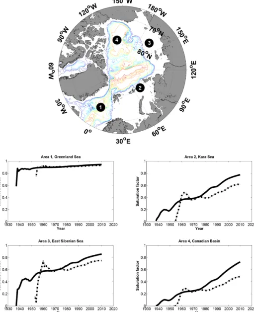
The surface saturations of transient tracers are influenced by sea surface temperature and salinity, ice coverage, wind speed, bubble effects, atmospheric growth rate of the tracer and the boundary dwell time of the water parcel (i.e., the time the water parcel is in contact with the atmosphere). How- ever, the saturation state of transient tracers at the air–sea interface before, during and after water mass formation is rarely known, since water mass formation generally occurs in winter at high latitudes, which renders it almost impossi- ble to obtain measurements. Shao et al. (2013) provide modeled data of monthly surface saturations of CFC-11, CFC-12 and SF₆ from 1936 to 2010 on a global scale. This model output can be used to estimate the tracer saturation ratio of different water masses by using the surface saturation of the specific formation area and yearly formation period. The formation types and areas are notably different for water masses that occur in the Fram Strait. The model output shows high variabilities in surface saturations at different formation sites, namely the Greenland Sea, the Arctic shelf regions and the Arctic open water (Fig. 8). In contrast, the tracer age rela-

CFC−12 Undersaturation

Tracer age (CFC−12) [yrs]

Tracer age (SF₆) [yrs]

0 10 20 30 40 50 60

15 20 25 30 35 40 45 50

SF6 Supersaturation

Figure 7. Relation between the IG-TTD-based tracer age relation- ship of the unity ratio (black line) and the mean tracer age relationship of the upper set of the field data (red line). The shape of both curves indicates similarities between the modeled and field data. The difference can be explained by undersaturation of CFC-12 and/or supersaturation of SF₆(see inset).

tionships of the two sets in Fig. 5 indicate relatively similar deviations in saturation. The complex boundary conditions in the Arctic, e.g., possible gas exchange through ice cover and the changing extent of the ice cover, might bias the results of the saturation model. Therefore, we only used the surface saturation of the Greenland Sea (Area 1 in Fig. 8) which agrees with the findings of Tanhua et al. (2008) who used available field data to investigate historic tracer saturations. The IG-TTD-based mean age provides the link between the observed tracer concentrations and the corresponding time-dependent saturation. Therefore, the saturation cor- rections were applied to the atmospheric history (boundary conditions) of each tracer. These new boundary conditions are then applied to the measured tracer concentrations and the IG-TTD which then yields a saturation-corrected mean age. This mean age in turn can then be used to back-calculate the saturation-corrected tracer concentrations using the orig- inal (uncorrected) boundary conditions.

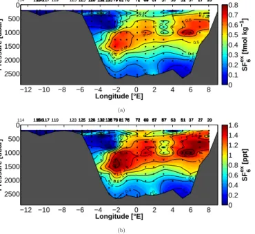
The SF6 excess is estimated using the corrected CFC- 12 concentrations and the IG-TTD (1/ 0=1.0) to calculate theoretical SF6 concentrations of the water parcel, i.e., back-calculated SF6concentrations. The difference between the theoretical SF6concentration and the measured SF6con- centration denotes the SF₆ excess in the water. Note that this SF₆ excess is based on the assumption that the IG- TTD and unity ratio describe the prevailing ventilation pattern of the water masses. Figure 9 shows the SF₆ excess in fmol kg⁻¹ and ppt for depths below 200 m. This upper depth limit is invoked by the fact that CFC-12 concentrations above the current atmospheric concentration limit cannot be applied to the IG-TTD. The SF₆excess is much higher (0.5–0.8 fmol kg⁻¹/1.0–1.6 ppt) for northward-propagating water masses compared to water masses of Arctic origin (0–

(8)

Figure 8. Surface saturations of CFC-12 (black solid line) and SF₆(black dash-dotted line) based on the model output of Shao et al. (2013).

The model output shows mean values of the corresponding grids with a dimension of 300×300 nm for typical source regions of the following different water mass types: (1) the Greenland Sea, (2–3) Arctic shelf regions and (4) Arctic open water/fast-ice region.

0.4 fmol kg⁻¹/0–0.8 ppt). There are at least two possible effects which can cause such significant supersaturations of SF₆.

One possibility refers to the deliberate tracer release experiment in 1996 where 320 kg (∼2190 mol) of SF₆were introduced into the central Greenland Sea (Watson et al., 1999).

The patch was redistributed by mixing processes and entered the Arctic Ocean via the Fram Strait and Barents Sea Open- ing and the North Atlantic via Denmark Strait and the Faroe Bank Channel (Olsson et al., 2005; Tanhua et al., 2005; Mar- nela et al., 2007). Assuming that 50−80 % of the deliberately released SF6still remains in the Nordic Seas and the Arctic Ocean (1095–1752 mol) and that 10− −50 % of the corresponding total water volume of 1.875×10¹⁸–9.375×10¹⁸L

(Eakins and Sharman, 2010) is affected, a mean offset of 0.12–0.93 fmol L⁻¹might be found. This mean offset is in the range of the observed SF₆excess concentrations. How- ever, CFC-12 and SF₆data of the Southern Ocean (Stöven et al., 2015) show similar tracer age relationships compared to the Fram Strait data but with no influence of deliberately released SF₆. This indicates that another source of excess SF₆ may exist which is much larger than the source of the tracer release experiment.

Liang et al. (2013) introduced a model which estimates supersaturations of dissolved gases by bubble effects in the ocean. This model predicted an increasing supersaturation for increasing wind speed and decreasing temperature, i.e., the bubble effect becomes more significant at high latitudes.

(9)

−12 −10 −8 −6 −4 −2 0 2 4 6 8 0

500 1000 1500 2000 2500

0.1

0.1 0.1

0.1

0.2

0.2 0.2

0.3

0.3 0.3

0.4 0.3 0.4

0.4 0.4

0.4

0.5 0.5

0.5

0.5 0.6 0.6

0.6

0.7 114 115115115115106106106117117117 119119 123123 125125125125 128128128128128128128 132132132132132132132132132132132 135135135135135135135135135135135135 79 79 79 79 79 79 79 79 79 79 81 81 81 81 81 81 81 81 76 76 76 76 76 76 76 76 76 76 72 72 72 72 72 72 72 72 72 72 69 69 69 69 69 69 69 69 69 69 67 67 67 67 67 67 67 67 67 67 57 57 57 57 57 57 57 57 57 57 57 53 53 53 53 53 51 51 51 51 51 51 51 37 37 37 37 27 27 27 27 27 20 20 20 20

Longitude [°E]

Pressure [dbar] SF6ex [fmol kg−1]

0 0.1 0.2 0.3 0.4 0.5 0.6 0.7 0.8

(a)

−12 −10 −8 −6 −4 −2 0 2 4 6 8

0 500 1000 1500 2000 2500

0

0 0

0

0.2

0.2 0.2

0.2

0.4

0.4 0.4

0.4

0.4 0.6

0.6

0.6 0.6

0.8

0.8 1 0.8

1

1 1

1

1.2 1.2

1.2

1.2 1.4

1.4

1.6

114 115115115115106106106117117117 119119 123123 125125125125 128128128128128128128 132132132132132132132132132132132 135135135135135135135135135135135135 79 79 79 79 79 79 79 79 79 79 81 81 81 81 81 81 81 81 76 76 76 76 76 76 76 76 76 76 72 72 72 72 72 72 72 72 72 72 69 69 69 69 69 69 69 69 69 69 67 67 67 67 67 67 67 67 67 67 57 57 57 57 57 57 57 57 57 57 57 53 53 53 53 53 51 51 51 51 51 51 51 37 37 37 37 27 27 27 27 27 20 20 20 20

Longitude [°E]

Pressure [dbar] SF6ex [ppt]

0 0.2 0.4 0.6 0.8 1 1.2 1.4 1.6

(b)

Figure 1

Figure 9. Distribution of SF₆ excess (a) concentrations in fmol kg⁻¹ and (b) partial pressures in ppt. The upper 200 m and station 15 cannot be calculated due to the atmospheric concentration limit of CFC-12 which inhibits an application of the IG-TTD.

Furthermore, Liang et al. (2013) show that the magnitude of supersaturation depends on the solubility of the gas. The less soluble a gas, the more supersaturation can be expected.

Supporting this, Stöven et al. (2015) describe surface measurements of SF6and CFC-12 directly after heavy wind conditions in the Southern Ocean where SF6 supersaturations of 20–50 % could be observed. The CFC-12 concentrations were only affected to a minor extent which can be explained by the differences in solubility. This bubble-induced supersaturation can also be expected to occur during the process of water mass formation in the Greenland Sea, which usually occurs during late winter, i.e., during a period with low surface temperatures and heavy wind conditions. Further- more, the maximum SF₆ excess in the Arctic Intermediate Water layer in Fig. 9 and the generally elevated tracer concentrations of CFC-12 and SF₆in the same area (see Fig. 3) reaffirm the assumption of bubble-induced supersaturation of SF6. However, this hypothesis stands in opposition to the current assumption that trace gases are generally undersaturated during water mass formation (Tanhua et al., 2008; Shao et al., 2013).

Future investigations are necessary to determine the different impact of under- and supersaturation effects on soluble gases at the air–sea interface. It can be expected that possible scenarios are not restricted to distinct saturation states any longer but rather comprise mixtures of equilibrated, under- and supersaturated states of the different gases.

Table 1. Mean (± standard deviation) concentrations of anthropogenic carbon (Cant) and mean age in the Fram Strait, separated in water mass types.

Water mass Cant Mean age

(µmol kg⁻¹) (years)

AW/RAW 50 (±6) 9 (±10)

PSWw 46 (±5) 9 (±10)

PSW 43 (±2) 7 (±6)

AAW 38 (±5) 32 (±15)

AIW 31 (±5) 54 (±20)

uPDW 28 (±4) 69 (±19)

NDW 18 (±4) 143 (±44)

CBDW 15 (±2) 173 (±23)

EBDW/GSDW 11 (±1) 254 (±32)

3.5 Anthropogenic carbon and mean age

Since CFC-12 is not affected by tracer release experiments, and possibly only to a minor extent by bubble effects, we used this tracer to calculate the mean age of the water and the corresponding anthropogenic carbon content. SF₆ was only used in the surface and upper halocline, i.e., where CFC- 12 exceeds the atmospheric concentration limit of 528 ppt and where effects of SF6supersaturation are comparatively small. Saturation-corrected tracer data were applied for sub- surface data below 200 m whereas surface data were found to be near equilibrium state with the atmosphere. Figure 10 shows the anthropogenic carbon distribution and Fig. 11 shows the mean age of the water masses. As expected from the relation between transient tracers, mean age and anthropogenic carbon, the distribution patterns are similar to that of transient tracers. The highest anthropogenic carbon concentrations of 50–55 µmol kg⁻¹were found in the upper 600 m of the Atlantic Water/Recirculating Atlantic Water and slightly lower concentrations of 40–45 µmol kg⁻¹in the Po- lar Surface Water/warm Polar Surface Water layer. The mean age of these water masses is 0–20 years. Note that these water layers show the highest mean current velocities in the Fram Strait (Beszczynska-Möller et al., 2012). The area of the tracer maximum at 1–3^◦W shows elevated concentrations of 35–40 µmol kg⁻¹ and a mean age of 20–40 years. The remaining water layers below 600 m show anthropogenic carbon concentrations lower than 35 µmol kg⁻¹ with decreasing concentrations with increasing depth; anthropogenic carbon is comparatively low (<10 µmol kg⁻¹) in deep water masses such as Canadian Basin Deep Water and Eurasian Basin Deep Water/Greenland Sea Deep Water. Accordingly, the mean age increases with increasing depth from 30 years to 280 years and shows a maximum mean age of 286 years in the bottom layer at the prime meridian. Table 1 shows the mean values and standard deviation of each specific water layer.