Seasonal variability of Atlantic Water recirculation in Fram Strait from observations

(1)

Seasonal variability of Atlantic Water recirculation in Fram Strait

from observations

Zerlina Hofmann

1010110

First supervisor: Prof. Dr. Peter Brandt Second supervisor: Dr. Wilken-Jon von Appen

A thesis presented for the degree of Master of Science in Climate Physics: Meteorology and Physical Oceanography

Faculty of Mathematics and Natural Sciences Christian-Albrechts-Universit¨ at zu Kiel, Germany

February 24, 2020

(2)

(3)

Abstract

This account of the first direct long-term observations of the Atlantic Water recirculation in Fram Strait gives new insight to both the recirculation’s location and variability. While Fram Strait is largely influenced by the inflow of warm, saline water from the Atlantic Ocean and the outflow of cold, fresh water and sea ice from the Arctic Ocean, part of the Atlantic Water inflow recirculates, i.e. turns westward in Fram Strait already. This affects both the amount of heat that is transported to the Arctic Ocean, as well as the properties of water that ultimately contributes to deep water formation in the Nordic Seas, an important aspect of the overturning circulation of the world’s oceans.

We investigate the Atlantic Water recirculation with regard to its location and variability by analysing observations from an array of five moorings. The moorings were placed at an equal distance of 40’ of latitude between 78^◦10’N and 80^◦50’N along the prime meridian, and were in the water from August 2016 to July 2018, where they measured temperature, salinity, and velocity in the upper 800 m of the water column.

We can confirm the existence of two recirculation branches with distinct properties north (in the vicinity of 80^◦10’N) and south (in the vicinity of 78^◦50’N) of the Molloy Hole, and observe no recirculation at the northernmost mooring (80^◦50’N).

The southern recirculation branch is present throughout the year, as indicated by strong westward velocities, and relatively high temperatures and salinities (that is, higher than further north and south). It displays stronger velocities during the first half of the year with a maximum in May and a strong additional northward component in March to May. At times, it affects the mooring locations further south and north, indicating some meandering or broadening/narrowing of the flow.

The northern recirculation branch is much stronger in winter and nearly absent in summer, as indicated by a strong temperature and salinity maximum in Decem- ber to February, and a minimum in June to August. While southward velocities suggest the corresponding mooring to be located in the Arctic Ocean outflow, the variability of the velocities is high, and eddy kinetic energy is maximal in November, and January/February. This highlights the importance of eddies for the northern recirculation branch. It may affect the mooring location further south by blocking southward transport of Polar Water at the prime meridian during its presence, and instead promoting the southward transport of Atlantic Water.

New insights on the two recirculation branches carrying Atlantic Water constrain the dynamics that take place in Fram Strait. This knowledge can improve conceptual as well as numerical models of how the role of Fram Strait as a connection between the Nordic Seas and the Arctic Ocean, and its part in the overturning circulation will evolve in the future.

(4)

(5)

Zusammenfassung

Dieser Bericht der ersten direkten Langzeit-Messungen der Rezirkulation atlantischen Wassers in der Framstraße gibt neue Einblicke bezüglich der Lage und Vari- abilität der Rezirkulation. Die Framstraße ist vornehmlich durch den Zustrom war- men, salzigen Wassers aus dem Atlantischen Ozean und den Ausstrom kalten, süßen Wassers vom Arktischen Ozean beeinflusst. Bereits in der Framstraße rezirkuliert jedoch ein Teil des Atlantischen Wassers, das heißt er biegt Richtung Westen in die zentrale Framstraße ab. Das hat Einfluss sowohl auf den Umfang der Wärme, die in Richtung des Arktischen Ozeans transportiert wird, als auch auf die Eigenschaften des Wassers, das letztlich zur Tiefenwasserformation der Nordmeere beiträgt und zu einem Teil der Umwälzzirkulation der Weltmeere wird.

Wir untersuchen die Rezirkulation Atlantischen Wassers bezüglich seiner Lage und Variabilität, indem wir Beobachtungen von einer Verankerungsreihe analysieren. Die Verankerungsreihe besteht aus fünf Verankerungen, die in gleicher Entfernung von 40’ Breite zwischen 78^◦10’N und 80^◦50’N entlang des Nullmeridian platziert wur- den. Sie waren von August 2016 bis Juli 2018 im Wasser und maßen Temperatur, Salzgehalt und Strömungsgeschwindigkeit in den oberen 800 m der Wassersäule.

Wir können bestätigen, dass zwei Rezirkulationspfade mit ausgeprägten Eigen- schaften nördlich (in der Nähe von 80^◦10’N) und südlich (in der Nähe von 78^◦50’N) des Molloytiefs existieren. An der nördlichsten Verankerung (80^◦50’N) beobachten wir keine Rezirkulation.

Der südliche Rezirkulationspfad ist das ganze Jahr vorhanden, gekennzeichnet durch starke westwärtige Geschwindigkeiten und hohe Temperatur und Salzgehalt (im Vergleich zu weiter nördlich oder südlich). Die westwärtigen Geschwindigkeiten sind stärker während der ersten Hälfte des Jahres, mit einem Maximum im Mai und zusätzlich einer starken nordwärtigen Strömungskomponente im März bis Mai.

Bisweilen beeinflusst der südliche Rezirkulationspfad die Verankerungen weiter südlich oder nördlich, was auf Mäandern oder eine Ausdehnung/Verengung der Strömung hindeuten könnte.

Der nördliche Rezirkulationspfad ist deutlich stärker im Winter und ist beinahe abwesend im Sommer, worauf ein klares Temperatur- und Salzgehaltsmaximum im Dezember bis Februar und ein Minimum im Juni bis August hindeutet. Die südwärtigen Geschwindigkeiten an der zugehörigen Verankerung deuten zwar darauf hin, dass die Verankerung sich im Ausstrom des Arktischen Ozeans befindet, aber die Variabilität der Geschwindigkeiten ist hoch, und die kinetische Energie von Ozeanwirbeln ist maximal im November und Januar/Februar. Das hebt die Bedeutung von diesen Ozeanwirbeln für den nördlichen Rezirkulationspfad hervor.

Er beeinflusst möglicherweise die Gegend weiter südlich, indem er den südwärtigen Transport von Polarem Wasser blockiert und stattdessen den südwärtigen Transport von Atlantischem Wasser fördert.

(6)

Neuen Erkenntnisse zu den beiden Rezirkulationspfaden, die Atlantisches Wasser transportieren, engen unser Verst¨andnis zur Dynamik in der Framstraße weiter ein.

Dieses Wissen kann einen Beitrag zur Verbesserung von konzeptuellen sowie nu- merischen Modellen leisten, im Bezug darauf wie sich die Framstraße als Verbindung zwischen den Nordmeeren und dem Arktischen Ozean, sowie als Anteil an der Umw¨alzzirkulation, in Zukunft entwickeln wird.

(7)

List of Figures

1.1 Schematic circulation of the Nordic Seas . . . 2

1.2 Map of Fram Strait with bathymetry . . . 3

1.3 Map of Arctic Ocean inflow and recirculation pathways fromHatter- mann et al. (2016) . . . 8

2.1 Map of central Fram Strait with mooring locations . . . 15

2.2 Gridded zonal velocity section with instrument locations in the water column . . . 16

2.3 Potential temperature - Salinity plot with linear regression at R3-1 and R4-1 . . . 17

2.4 Percentage of gridded measurements that fit different water mass definitions . . . 21

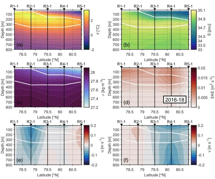
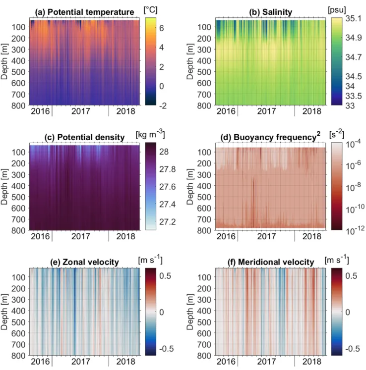
3.1 Gridded sections of different variables, averaged over the entire time series . . . 24

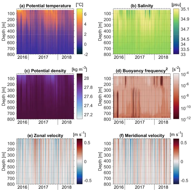
3.2 Hovm¨oller diagrams of different variables at R1-1 . . . 25

3.3 As in Figure 3.2, but at R2-1 . . . 26

3.4 Map of Fram Strait with sea ice concentration (80% and 20%) in February and August . . . 28

3.8 Seasonal cycle of water mass layer thickness . . . 34

3.9 Seasonal cycle for different variables from all gridded measurements . 35 3.10 Same as Figure 3.9, but only for gridded measurements that fit the AW definition . . . 36

3.11 Same as Figure 3.9, but only for gridded measurements that fit the AAW definition . . . 37

3.12 Same as Figure 3.9, but only for gridded measurements that fit the DW definition . . . 38

3.13 Monthly averages of potential temperature and eddy kinetic energy at R1-1 . . . 40

3.14 Monthly averages of potential temperature and salinity at R5-1 . . . 42

3.15 Mean velocity and standard deviation ellipses from moored instruments in the upper water column . . . 44

3.16 Monthly averages of zonal and meridional velocity at R2-1 . . . 45

3.17 Seasonal cycle of the eddy kinetic energy at R moorings . . . 47

3.18 Seasonal cycle of the eddy kinetic energy fromvon Appen et al. (2016) 48 3.19 Monthly averages of salinity and eddy kinetic energy at R4-1 . . . 49

(10)

3.20 Zonal velocities and eddy kinetic energy of eastward/westward spells 51 3.21 Monthly averages of potential temperature and eddy kinetic energy

at R3-1 . . . 53 3.22 First empirical orthogonal function and principal component of po-

tential temperature . . . 54 3.23 Simulated velocity from simulation FESOM 1km in the Nordic Seas . 55 B.1 Potential temperature - Salinity plot with linear regression of the two

lower CTDs . . . 78 C.1 Seasonal cycle for standard deviation of different variables from all

gridded measurements . . . 79 C.2 Same as Figure C.1, but only for gridded measurements that fit the

AW definition . . . 80 C.3 Same as Figure C.1, but only for gridded measurements that fit the

AAW definition . . . 81

(11)

List of Tables

2.1 Water mass definitions after Rudels et al. (2005) . . . 20 A.1 Meta data of the moorings . . . 74 A.2 Meta data of the instruments . . . 75

(12)

(13)

Chapter 1 Introduction

The Arctic Ocean is mostly surrounded by landmass, though exchange of water and sea ice is possible through a few pathways, namely the Fram Strait, the Barents Sea Opening, the Bering Strait, and various small channels in the Canadian Arctic Archipelago. The Fram Strait is the only deep connection (∼2500 m) between the Arctic Ocean and the Nordic Seas. Warm, saline water from the Atlantic Ocean enters via the West Spitsbergen Current (WSC) on the eastern side of the strait, while cold, fresher water and sea ice (as well as modified, previously warm and saline water) from the Arctic Ocean exits via the East Greenland Current (EGC) on the western side. The circulation in the Fram Strait is strongly defined by these boundary currents importing and exporting water to and from the Arctic Ocean.

Part of the Atlantic Water (AW), however, recirculates (i.e. turns westward) in the Fram Strait before ever reaching the Arctic Ocean. This westward flow component, the recirculation of AW in Fram Strait, will be the focus of this thesis. In the following, we will introduce the general setting of the Nordics Seas and Fram Strait in particular (Chapter 1.1), summarise the research status on the AW recirculation (Chapter 1.2), highlight its importance on a larger scale (Chapter 1.3), and formulate the research questions that will be answered in this thesis (Chapter 1.4).

1.1 Fram Strait and the surrounding seas

The so-called Arctic Mediterranean includes both the Nordic Seas and the Arctic Ocean and their adjacent shelf areas, with the two being connected via Fram Strait and the Barents Sea (Figure 1.1). The Fram Strait is the ocean passage between Greenland and the Svalbard archipelago, located roughly at 76–82^◦N and centred on the prime meridian. The Barents Sea is a marginal sea of the Arctic Ocean, located off the northern coasts of Scandinavia and Russia, and fairly shallow (∼230 m). The Nordic Seas comprise the Greenland Sea, the Norwegian Sea, and the Iceland Sea (Figure 1.1) and are bounded to the south by the Greenland-Scotland-Ridge, which spans from Greenland over Iceland and the Faroe Islands to Shetland (Scotland).

On average, it is only 500 m deep, with some parts reaching a depth of 850 m.

The Fram Strait is thus of particular importance in its role as the deep connection between the Arctic Ocean and the Nordic Seas.

The deep part of the strait horizontally spans about 300 km, bordered by the broad continental shelves of Greenland (∼300 km) and Svalbard (∼50 km). The topography in the centre of the strait is thus characterised by continental slopes in the east

(14)

1.1. FRAM STRAIT AND THE SURROUNDING SEAS

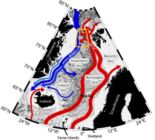
Figure 1.1: Schematic circulation of the Nordic Seas with inflow from the Atlantic Ocean in red and outflow from the Arctic Ocean in blue. Different shadings of blue indicate different amounts of mixing between warm, saline AW and cold, fresh PW. The yellow box marks the study area.

Abbreviations are as follows: NwAC = Norwegian Atlantic Current, WSC = West Spitsbergen Current, EGC = East Greenland Current, NIIC = North Iceland Irminger Current, NIJ = North Icelandic Jet.

and west, as well as some complex topography in between. The latter largely takes shape as the Knipovich Ridge, the northernmost section of the Mid-Atlantic Ridge that connects with the Gakkel Ridge in the Arctic Ocean (Figure 1.2).

The so-called Yermak Plateau is a plateau of about 700 m depth that is located northwest of Svalbard. The average water depth in the deep part of the strait is about 2500 m, though the deepest part is a bathymetric feature called the Molloy Hole, more than twice as deep (5555 m, Figure 1.2). Two fracture zones enclose this area, the Spitsbergen Fracture Zone in the north and the Molloy Fracture Zone in the south. Parallel to the Molloy Fracture Zone further south, the Hovgaard Ridge and the East Greenland Ridge enclose the Boreas Abyssal Plain, a wider plain of about 2500 m depth. Between 71 to 75^◦N the Mohns Ridge and Knipovich Ridge split the Nordic Seas into the Greenland Abyssal Plain and the Lofoten Basin (Hansen and Østerhus,2000).

In the next subchapters, an introduction is given on the warm, saline inflow to, and the cold, fresh outflow from the Arctic Ocean and its path through the Nordic Seas (Chapters 1.1.1 and 1.1.2, respectively). Water masses that are transported to or formed in the Nordic Seas and the Arctic Ocean are explained in detail in Chapter 1.1.3.

(15)

Yermak Plateau

Spitsbergen FZ Boreas

Abyssal Plain Molloy FZ

Greenland Abyssal Plain

MH

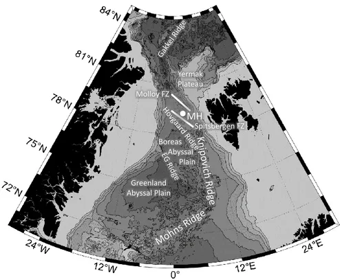
Figure 1.2: Map of Fram Strait with bathymetry from Schaffer et al.(2019) and bathymetrical feature names from the IHO-IOC GEBCO Gazetteer of Undersea Feature Names (https://www.

gebco.net). The white lines mark fracture zones, the white dot the Molloy Hole. Abbreviations are as follows: MH = Molloy Hole, FZ = Fracture Zone, EG = East Greenland.

1.1.1 Inflow

Warm, saline AW enters the Nordic Seas between Greenland and Scotland, origi- nating from two source regions. One is the area, where the North Atlantic Current enters the eastern Atlantic, feeding the inflow branches between Greenland and Iceland (the North Icelandic Irminger Current, NIIC), and between Iceland and the Faroe Islands (Hansen and Østerhus, 2000). The other is located south of the Greenland-Scotland inflow region just off the European shelf, feeding a current pass- ing through the Faroe-Shetland Channel (Hansen and Østerhus, 2000). The inflow between Iceland and the Faroe Islands is the western branch, the inflow through the Faroe-Shetland Channel the eastern branch of the Norwegian Atlantic Current (NwAC, Figure 1.1). Both are topographically steered through the Nordic Seas along the Mohns and Knipovich Ridge, and the Norwegian shelf edge, respectively. The eastern branch bifurcates north of Norway, with part of the current continuing into the Barents Sea (Orvik and Niiler, 2002). Both branches of the NwAC ultimately converge in the region west of central Spitsbergen as the WSC, with the shortest distance between the two branches being at 77^◦N due to bottom topography (Wal- czowski et al.,2005). In the northern Fram Strait the flow splits again (Figure 1.1).

It partly turns westward and recirculates, joining the EGC on its southward path, as described in much more detail in Chapter 1.2. The remainder of the flow splits into one branch following the coastline, cutting across the Yermak Plateau, and the other following the shelf break of the plateau (Perkin and Lewis, 1984; Quadfasel

(16)

et al., 1987; Walczowski et al., 2005). The two branches have been termed the Svalbard Branch and the Yermak Branch, respectively (Manley et al., 1992). The Yermak Branch splits up once more, partly progressing along the continental slope of the Yermak Plateau and partly crossing the Yermak Plateau through the Yermak Pass (Gascard et al., 1995), the latter having been named the Yermak Pass Branch (Koenig et al., 2017b). Model studies suggest the Yermak Pass Branch to have a strong seasonality and to be the dominant route for AW to enter the Arctic Ocean (Koenig et al.,2017a;Crews et al.,2019). While the Svalbard branch appears to be relatively stable throughout the year, in the model study byCrews et al.(2019), the WSC’s increased flow during the winter is divided between the recirculation and the Yermak Pass Branch. Owing to their origin from different branches of the NwAC, the Svalbard and Yermak branches have different signatures and different advection timescales from the splitting of the NwAC to the point, where they enter the Arctic Ocean, resulting in different cooling rates of the AW (Beszczynska-M¨oller et al., 2012). Substantial heat is lost from the Yermak Branch due to strong tidal currents over the Yermak Plateau that lead to increased turbulent mixing (Padman et al., 1992; Fer et al., 2015).

The most obvious characteristics of the WSC are its relatively high temperature and salinity, reflecting its origin far to the south (Hanzlick, 1983). Average northward transport values at 78.5^◦–79^◦N range from about 5–12 Sv (Aagaard et al., 1973;

Hanzlick,1983; Fahrbach et al., 2001; Schauer et al., 2004; Walczowski et al., 2005;

Beszczynska-M¨oller et al.,2012). Generally, direct current measurements yield much higher transports than hydrographic measurements and model studies (Walczowski et al., 2005). This is because the WSC has a strong barotropic component, and as a direct consequence, it strongly interacts with bottom topography (Hanzlick, 1983; Gascard et al., 1995). The WSC is barotropically and baroclinically unstable at least sometimes (Teigen et al., 2010, 2011). von Appen et al. (2016) found that the WSC is much more baroclinically unstable and likely to generate eddies during winter than during summer, while barotropic instability plays some role during winter in regions, where the topography supports it. The barotropic nature and the unsteadiness of the WSC, as well as the variable bottom topography in Fram Strait explain why the WSC has such a strong tendency to branch and form eddies along topographic fracture zones (Gascard et al., 1995).

An increase of the year-round mean AW temperature advected from the North Atlantic has been observed from 1997 to 2010 at the zonal array in Fram Strait (Beszczynska-M¨oller et al., 2012). This has been ongoing at a less steep rate since 2010 (W.-J. von Appen, pers. comm., 2019). In addition von Appen et al. (2015) found that the deep (>1000 m) water masses north and south of Fram Strait are warming, which will likely cause exchange processes at depth within the strait to change. Walczowski et al. (2017) also observed a clear increase in summer AW temperature in the whole layer from the surface down to 1000 m.

1.1.2 Outflow

The Arctic Ocean outflow in Fram Strait north of 80^◦N has been observed and modelled as a broad barotropic flow between the northeast Greenland shelf and 0^◦ and may at least partly be topographically steered (Richter et al., 2018). Further south the EGC follows the Greenland continental shelf break (Figure 1.1), contains

(17)

stronger velocities (Aagaard and Coachman,1968a;de Steur et al.,2014), and has a stronger baroclinic component (Aagaard and Coachman,1968b;Gascard et al.,1995;

Richter et al., 2018). Foldvik et al. (1988) found about half of the EGC transport at 79^◦N to be barotropic though, and de Steur et al. (2014) found the EGC to be even more barotropic at 78^◦50’N compared to 79^◦N. The study by de Steur et al.

(2014) may, however, have been influenced by a warm anomaly present at the time it was conducted. Both de Steur et al.(2014) and Richter et al. (2018) argue that the recirculating AW affects the EGC in its strength and structure. Yearly averaged southward transport values at 78^◦50’N range from about 4–15 Sv, and at 79^◦N from about 2–10 Sv (de Steur et al., 2014), though previous yearly averages from the same mooring array at 79^◦N are larger, between 11–13 Sv (Fahrbach et al., 2001;

Schauer et al., 2004), likely due to different data handling methods. In 1994–95 at 75^◦N a southward transport of 21 Sv was found — part of this transport must be waters that recirculate within the Greenland Sea Gyre, as well as waters that will exit the Greenland Sea further south (Woodgate et al., 1999).

H˚avik et al.(2017) found that the EGC has three distinct branches: the shelf break EGC flowing along the shelf break all the way from the Arctic Ocean outflow to the Denmark Strait, a jet carrying PW on the continental shelf south of 74^◦N, and the outer EGC over the mid- to deep continental slope fed by the recirculation (Figure 1.1). Both the outer EGC and the shelf break EGC flow towards the south side- by-side at least as far south as the Jan Mayen Fracture Zone (H˚avik et al., 2017).

Here the denser waters are likely deflected towards the east and circulate around the Greenland Sea Gyre (Figure 1.1), potentially penetrating towards the centre and interacting with the Greenland Sea waters (Rudels et al., 1999). The surface outflow of the EGC combined with the overflow across the Greenland-Scotland Ridge comprises the total outflow from the Arctic Mediterranean through the Greenland- Scotland gap (Hansen and Østerhus,2000). The Iceland Sea may also be a potential contributor to the overflow via the North Icelandic Jet (NIJ, Figure 1.1), which flows along the northern continental slope of Iceland (V˚age et al., 2013).

1.1.3 Water masses

Here, water masses are introduced in the context of their origin/formation, quanti- tative definitions of the water masses relevant to the data analysis in this thesis can be found in Table 2.1.

Water of Atlantic origin entering the Norwegian Sea between Iceland and Scotland, which is carried north by the NwAC, is termed Atlantic Water (AW), a surface water mass associated with a temperature and salinity maximum. Part of the AW enters the Barents Sea, where it loses a lot of heat to the atmosphere and gains salinity in the form of brine as ice forms, so that the water mass rapidly changes its characteristics (Jones, 2001). The remaining AW continues on its northward path with the WSC in Fram Strait, where it continuously loses heat, while freshwater is added, reducing its salinity (Piechura et al., 2001), or it recirculates and has been termed Return Atlantic Water (Mauritzen, 1996), or Recirculating Atlantic Water (Rudels et al.,2002). The amount of heat carried towards the Arctic Ocean that is vertically mixed from the WSC core towards the ice is enough to maintain essentially ice-free conditions west and north of Svalbard to 80^◦–82^◦N (Aagaard et al.,1987;Onarheim et al., 2014).

(18)

When the AW enters the Arctic Ocean, it is further modified by heat loss at the surface and by mixing with colder waters from the north. Nonetheless, it can still be identified by its relatively high temperature, which decreases both to the east and to the north (Perkin and Lewis, 1984). As one moves into the basin, the rate of reduction of the temperature decreases (Perkin and Lewis, 1984).

Inflow through the Bering Strait is comparatively small, but has been increasing in 2001–2014 from∼0.7 Sv to ∼1.2 Sv (Woodgate,2018). The water of Pacific origin that reaches the Arctic Ocean is at times stored in the Beaufort Gyre and eventually drained through the passages of the Canadian Arctic Archipelago for the most part (Falck et al.,2005). Thus, the main water mass in the Arctic Ocean with which the AW can interact, either directly or through the melting and freezing of sea ice, is the fresh Polar Water (PW) added by river runoff, net precipitation, and ice melt

— it dilutes the AW and produces low density surface water, which is counteracted by cooling and freezing (Rudels and Quadfasel, 1991). At this point, the AW has been strongly modified and is traditionally referred to as Arctic Intermediate Water, though AIW is defined such that it also includes most of the intermediate water in the Greenland and Iceland Seas as well. For more clarity, the AIW that exclusively stems from the Arctic Ocean has been termed Arctic Atlantic Water (AAW) (Mau- ritzen,1996), though sometimes it is also referred to as Modified Atlantic Water (e.g.

Rudels and Quadfasel, 1991). In general, the Arctic Ocean can be characterised by a mixed layer consisting of PW at the surface and a cold halocline separating this surface layer from the warm layer of AW (Rudels, 1986). Below resides upper Polar Deep Water (characterised by a negative potential temperature-salinity relationship), which extends to an average depth of the Lomonosov Ridge (∼1700 m, the mid-ocean ridge running from northern Greenland to the Siberian shelf, separating the Arctic Ocean into the Eurasian and Amerasian Basins). Even further down in the water column, deep waters extends to a depth of about 2500 m, and beneath lies bottom water (Jones,2001). The deep water masses of the Arctic Ocean can mainly be separated by the major basins into Canadian Basin Deep Water and Eurasian Basin Deep Water (Rudels,1986).

The Arctic Ocean outflow with the EGC contains three major water masses: the cold and fresh PW at the surface with a strong halocline, the AW (depending on the latitude and the EGC branch more recirculated AW or AAW) with a temperature maximum and increasing salinity down to/around this maximum (below salinity is fairly constant), and cold, saline deep water furthest down (Aagaard and Coachman, 1968a). The intermediate and deep waters present in the Nordic Seas originate from the Arctic Ocean, and are mixed with deep waters from the Greenland Sea (i.e. Greenland Sea Deep Water, produced by open ocean deep convection) and the Norwegian Sea (i.e. Norwegian Sea Deep Water, a mixture of Arctic Ocean deep waters and GSDW), as well as intermediate waters from the Iceland Sea (Rudels and Quadfasel, 1991). Early studies mainly considered these deep water masses to contribute to the water that ultimately spills over the Greenland-Scotland-Ridge, either through the Denmark Strait as Denmark Strait Overflow Water or between Iceland, the Faroe Islands, and Shetland as Iceland Scotland Overflow Water (Swift et al., 1980; Rudels and Quadfasel, 1991). However, Mauritzen (1996) found that an alternative circulation scheme might be more likely, in which AW gradually becomes more dense (most prominently in the Norwegian Sea) and is transported by the boundary currents surrounding the Nordic Seas. More recently, the two main

(19)

1.2. RECIRCULATION IN FRAM STRAIT

sources of DSOW were found to be the EGC (both the shelf break and outer EGC branches) and the NIJ (Harden et al., 2016). The recirculated AW is thought to travel relatively unperturbed with the EGC along the continental slope of Greenland towards the Denmark Strait, exiting as the deepest water mass of the EGC above sill depth (Mauritzen, 1996;Rudels et al., 2002; H˚avik et al., 2017).

1.2 Recirculation in Fram Strait

First hints of a recirculation in Fram Strait were noted by Aagaard and Coachman (1968b), using observational data from 1958 and 1962, which showed a westward movement of warm water from the WSC north of 75^◦N. Perkin and Lewis (1984) found the indication of strong time-varying currents in the central Fram Strait during CTD measurements in 1981 that suggested some form of mixing between the WSC and the EGC. Since 1997 a mooring array has been deployed from the eastern Greenland shelf break to the western shelf break off Spitsbergen, with its eastern part located at 78^◦50’N and its western part at 79^◦N (Fahrbach et al., 2001). In 2002 the western part was moved to 78^◦50’N in order to line up with the rest of the array (de Steur et al., 2014), and since 2016 the eastern part has been moved to 79^◦N (von Appen,2018). In the following, this mooring array will be referred to as

’zonal array’.

Measurements at the latitude of the zonal array also indicate mostly westward flow in the central Fram Strait (Schauer et al., 2004; Beszczynska-M¨oller et al., 2012).

Other observations that have been used for a better understanding of the recirculation include in particular the Marginal Ice Zone Experiment (Johannessen, 1987;

Johannessen et al., 1987; Quadfasel et al., 1987; Gascard et al., 1988), and many CTD measurements (e.g. Manley, 1995; Marnela et al., 2013; Richter et al., 2018), yet long-term measurements in the central Fram Strait remain scarce, particularly during winter time. In the north, the ice cover further complicates observations.

In- and outflow through Fram Strait via the boundary currents has been simulated with different model setups (Schlichtholz and Houssais, 1999a,b; Maslowski et al., 2004; Losch et al., 2005; Aksenov et al., 2010; Fieg et al.,2010;Ilicak et al., 2016), and whether the resulting transports compare well to observations largely depends on whether the recirculation of AW in Fram Strait is well represented. More recently, several modelling setups have been utilised to evaluate the recirculation more closely (Kawasaki and Hasumi,2016;Hattermann et al.,2016;Wekerle et al.,2017;Richter et al., 2018), but the results are still inconclusive about location and strength of individual pathways, the northern limit of the recirculation, and the strength of the boundary currents. One of the main issues is the resolution necessary to resolve eddies that play a large role in Fram Strait (Rudels, 1987; Gascard et al., 1988, 1995; Rudels et al., 2005). The horizontal scale of eddies is governed by the local internal Rossby radius of deformation (Fieg et al., 2010), which is about 2–6 km in the WSC (von Appen et al., 2016) and about 6 km in the EGC (Zhao et al.,2014).

Only recent modelling efforts in the Fram Strait can be considered eddy-resolving (Kawasaki and Hasumi,2016;Hattermann et al.,2016;Wekerle et al.,2017;Richter et al., 2018).

Since the first measurements by Aagaard and Coachman (1968b), a lot of publications (as detailed below) have touched on the subject of AW recirculation in the Fram Strait, but a consensus on location, properties, and strength of this flow does

(20)

not yet exist.

1.2.1 Location

In terms of location of the recirculation there have been observations of AW and/or westward motion in the central Fram Strait between 75^◦N (Bourke et al.,1987) and as far north as 82^◦N (Gascard et al.,1995). Most of the recirculation appears to occur between 78^◦N and 80^◦N, in particular along the Spitsbergen Fracture Zone and south of the Molloy Hole (Quadfasel et al., 1987;Gascard et al., 1988,1995; Rudels et al.,2005;Richter et al.,2018), as well as along the Molloy Fracture Zone and north of the Molloy Hole (Bourke et al.,1988;Quadfasel et al.,1987;Richter et al.,2018).

High-resolution simulations of AW circulation in Fram Strait reveal a similar picture:

westward flow occurs both along the Spitsbergen Fracture Zone and along the Mol- loy Fracture Zone (Schlichtholz and Houssais,1999a,b;Kawasaki and Hasumi,2016;

Hattermann et al., 2016; Wekerle et al., 2017) and appears to be topographically steered along the Knipovich Ridge (Aksenov et al., 2010; Kawasaki and Hasumi, 2016;Wekerle et al.,2017). The two recirculation branches may even originate from the two different branches of the NwAC (Figure 1.3). Wekerle et al. (2017) addi- tionally found westward flow between 80^◦30’N and 81^◦30’N in their model, similar to observations from Gascard et al.(1995).

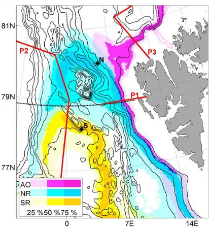
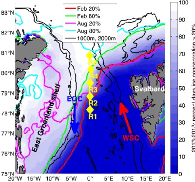
Figure 1.3: Map of the relative trajectory density distribution of floats of the southern recirculation (SR, yellow), northern recirculation (NR, blue), and Arctic Ocean inflow (AO, pink) pathway groups, being defined by the sections P1–P3 and shown as the percentage of all floats within each group. Figure fromHattermann et al.(2016).

The northern boundary of the recirculation remains unclear —Richter et al.(2018)

(21)

speculated, whether they observed the northern rim of the recirculation in their synoptic observations as they did not observe any AW at 80^◦48’N, though their model suggested the northern rim to lie further north. Generally, models with lower resolutions have produced a recirculation that takes place further south than observed (Fieg et al., 2010), though Wekerle et al. (2017) compared two models of different resolution and the low-resolution model only simulated recirculation too far north (between 80^◦N and 81^◦30’N). If the recirculation is simulated too far south or north, the boundary current transports in Fram Strait will not be represented correctly, and the central Fram Strait is left with a temperature bias.

The process of AW subducting below the PW in the western part of the strait will then also be misrepresented, potentially leading to AW properties along the Greenland continental margin.

Related to the northern extent of the recirculation it is interesting to consider, how large of a contributor the Yermak branch of the WSC is to the recirculating AW.

This, again, is far from clear: Aagaard et al. (1987) found that the Yermak Branch does not re-appear on the southeastern flank of the Yermak Plateau, suggesting it is mainly delivered to the Arctic Ocean, while Manley(1995) speculated that most, if not all of the Yermak Branch could be defined as recirculating. More recently,Crews et al. (2019) found that the properties of the WSC are associated with conditions that either promote flow onto the Yermak Plateau (a warmer, faster WSC), or flow deflecting from the continental slope, i.e. recirculation (a colder, slower WSC).

The recirculation, or at least part of it, has also frequently been described as the Return Atlantic Current (RAC), a current that lies along the front between the PW of the EGC and the AW present towards the east (Paquette et al., 1985). It occupies depths roughly between 50 and 400 m (Paquette et al.,1985;Bourke et al., 1987, 1988), is characterised by a subsurface temperature and salinity maximum (Paquette et al., 1985; Quadfasel et al., 1987), and is essentially all AW that has cooled with little or no dilution (Bourke et al.,1987,1988). It is described as a multi- path current (Gascard et al.,1995) or broken into differing filaments (Paquette et al., 1985), though the wording may suggest the RAC to be a constant stream or current.

Hence, the term RAC is used less often in publications that are more recent.

1.2.2 Properties

There has been clear evidence of eddies in the central Fram Strait (Rudels, 1987;

Gascard et al., 1995; Rudels et al., 2005; von Appen et al., 2018), which are likely generated along the continental slope off Spitsbergen in the WSC (Gascard et al., 1988, 1995). Instead of a continuous stream, the recirculation may solely exist as westward propagating WSC eddies (Gascard et al.,1988;Rudels et al.,2005), though these may be advected by a background flow (Johannessen et al., 1987). Model studies support the fact that there seems to be an abundance of mesoscale eddies and filaments in the flow within Fram Strait (Hattermann et al., 2016; Kawasaki and Hasumi, 2016). Besides in the WSC,Wekerle et al.(2017) found high values of eddy kinetic energy (EKE) between the northern rim of the Boreas Abyssal Plain and the Molloy Hole, and along the EGC and in the western part of the Boreas Abyssal Plain.

The eddies have been observed to mainly be composed of warm and salty AW (Gascard et al., 1995), but even if the recirculation only takes a short additional

(22)

northward excursion, the water loses a considerable amount of heat (Schauer et al., 2004). Simulations suggest that both warm-core anticyclonic eddies and cold-core cyclonic eddies are present in Fram Strait (Wekerle et al., 2017), which are then advected all the way to the EGC (Hattermann et al., 2016). When they reach western Fram Strait, they are potentially subject to mixing with the AAW carried by the EGC (Gascard et al.,1995;Rudels et al.,2005). How much heat the recirculated AW may add to the EGC has been documented byde Steur et al.(2014), when they looked at temperature measurements from the zonal array in Fram Strait, before and after the western part was moved from 79^◦N to 78^◦50’N. Temperatures at almost all mooring longitudes in the western part of the Fram Strait were higher at 78^◦50’N than at 79^◦. The westward velocity of the eddies was reported as about 0.05 m s⁻¹ (Gascard et al., 1988, 1995), while velocities of up to 0.13 m s⁻¹ were measured in the RAC (Bourke et al., 1988). The structure of the recirculation in an inverse model study was suggested to be mostly baroclinic south of the Molloy Hole and along the EGC, and mostly barotropic north of the Molloy Hole (Schlichtholz and Houssais, 1999a).

1.2.3 Transport

Transport estimates of the recirculation can be difficult to compare, as they include direct measurements of transports across the Fram Strait, inferred transports from measuring in the boundary currents, measurements that cover only part of the recirculation, or include the transport of other water masses than AW. Early estimates based on geostrophic velocities computed from CTD sections taken in 1980, 1983, and 1988 during summer suggest that about 1 Sv of the northward flow of AW in the WSC recirculates, adding more than one third to the flow in the upper layers of the EGC (Rudels, 1987; Gascard et al., 1995). Bourke et al. (1988) also anal- ysed summer CTD sections (from 1985), but differentiated between recirculation south of 79^◦N, deduced from a reduction of the WSC of 0.8 Sv, and recirculation between 79^◦N and 81^◦N, where a net westward flow of 0.4 Sv was measured. The zonal array in Fram Strait has given some insights into year-round direct current measurements. Fahrbach et al. (2001) estimated a westward recirculation from the two central moorings at 78^◦50’N and 79^◦N of 2.6 Sv. Schauer et al. (2004) observed a southward transport of about 0.5 Sv west of the Yermak Plateau branch of the WSC that had a remarkably similar temperature compared to the northward flow, suggesting it took only a short excursion north and recirculated quickly. Af- ter the western part of the mooring array was moved to line up with the eastern part, de Steur et al. (2014) found that the recirculation adds about 2.7 Sv to the EGC between 78^◦50’N and 79^◦N. Summer meridional sections (from about 78^◦N to 80^◦N) have shown geostrophic transports between 0.4 and 2.3 Sv, with no difference between the northern and southern part of the section in two years and opposing transports in one year (Marnela et al.,2013). Implied transports from zonal sections indicated AW recirculation of about 2 Sv in three out of four years and almost no recirculation in the fourth year north of 79^◦N (Marnela et al., 2013).

In an inverse model study Schlichtholz and Houssais (1999a) found that the recirculation rate, implied from the decrease in WSC transport from south to north and the increase in EGC transport from north to south, amounts to 1.8 Sv on average between 77^◦36’N and 78^◦54’N, and 0.5 Sv between 78^◦54’N and 79^◦54’N. Further

(23)

1.3. LARGE SCALE IMPACT OF THE RECIRCULATION

north the decrease in WSC and increase in EGC were not consistent. Other estimates from simulations are 5.2 Sv, of which 2.7 Sv consist of water warmer than 2^◦C (Kawasaki and Hasumi, 2016), and 2.4 Sv (Wekerle et al., 2017).

1.2.4 Recirculation percentage

Previous studies mostly agree on the fraction of AW that recirculates, which is considered to be half of the AW entering the Fram Strait (Rudels,1987;Marnela et al., 2013;de Steur et al.,2014). Manley(1995) estimated that about 20% is recirculated with the RAC, while the Yermak branch is the main contributor to the recirculation further north, which would constitute about half of the AW being recirculated north of 79^◦N.

Modelling studies find similar values of about half of the AW entering Fram Strait recirculating (Kawasaki and Hasumi, 2016; Wekerle et al., 2017). Schlichtholz and Houssais (1999a) found that about 75% of the WSC inflow recirculates. Hatter- mann et al. (2016) differentiate between 60% recirculation in late winter/spring and 30% recirculation during summer (when the total AW inflow to Fram Strait is also weaker).

1.2.5 Variability

Particularly the different reports of location and transport of the recirculation in different years suggest some interannual variability, while the importance of eddy activity for the recirculation suggests significant mesoscale variability. Since most measurements in central Fram Strait were conducted during summer, and many are only synoptic, information about seasonal variability can only be deduced from observations of the boundary currents or models. de Steur et al. (2014) found that after the western part of the zonal array in Fram Strait was moved from 79^◦N to 78^◦50’N, the southward velocity displayed a clear seasonality, implying that the recirculation contributes the seasonal signal. von Appen et al. (2016) also used observations from the zonal array and found a strong seasonality of EKE in the WSC and the central Fram Strait, with the EKE maximum in the WSC observed during winter, and the EKE maximum in the central Fram Strait observed a little later in April. They suggest that the recirculation likely advects eddies across the Fram Strait during winter, while during summer the amplitudes of EKE are generally much weaker (von Appen et al.,2016). Modelling studies also find the highest values of EKE in the WSC and export of water westwards to be the strongest during winter (Hattermann et al., 2016; Wekerle et al., 2017). Wekerle et al. (2017) did not find all recirculation branches to be present during summer, when the circulation around the Molloy Hole was absent.

1.3 Large scale impact of the recirculation

Subsequently, the large scale impact of the recirculation is described. The recirculation has important implications for the heat transport towards the Arctic Ocean, as it ultimately determines, how much of the warm, saline inflow through Fram Strait actually reaches the Arctic Ocean (Chapter 1.3.1). Recirculating AW hence affects sea ice cover in the Arctic Ocean as well as in Fram Strait, and can even reach the

(24)

Greenland shelf and affect the Greenland ice sheet (Chapter 1.3.2). The part of the recirculating AW that joins the EGC on its southward path has an impact on deep water formation (Chapter 1.3.3) and the meridional overturning circulation of the World Ocean (Chapter 1.3.4).

1.3.1 Heat transport towards the Arctic Ocean

While the tropics receive an excess in shortwave radiation, the high latitudes actually lose heat to space and thus some heat needs to be transported poleward in the atmosphere and the ocean for an equilibrium to establish. The largest transport towards the Arctic Ocean occurs in the atmosphere and less than 10% of the heat transport required to balance the heat loss to space is provided by the oceanic heat transport towards the Arctic Ocean (Rudels, 2016). The dominant source for this heat transport is the inflow of AW combined with the export of PW and ice through Fram Strait (Schauer et al., 2004). Both the WSC in Fram Strait and the Barents Sea inflow carry a significant amount of heat, but the Barents Sea inflow loses most of its heat directly to the atmosphere in the southwestern Barents Sea (Smedsrud et al., 2010). The AW in the WSC is able to preserve its warm core, as the upper part of the AW becomes transformed into a fresher surface layer by melting sea ice and mixing with water of Arctic origin (Beszczynska-M¨oller et al., 2012). The heat carried by the WSC that reaches the Arctic Ocean is then lost mostly within the deep ocean (Rudels, 2016). This is of particular interest, if one considers that the AW transported towards the Arctic Ocean may be increasing in temperature, and perhaps also in volume (Beszczynska-M¨oller et al.,2012). Recirculating AW in Fram Strait significantly impacts the redistribution of oceanic heat between the Nordic Seas and the Arctic Ocean (Hattermann et al., 2016), ultimately determining how much of the heat carried by the WSC reaches the Arctic Ocean and how much joins the EGC on its southward path.

1.3.2 Sea ice and glacial melt

Diminishing sea ice plays a leading role in Arctic temperature amplification due to the surface albedo feedback (Screen and Simmonds, 2010) — sea ice has a much higher surface albedo than open water, meaning a decrease in sea ice extent causes further surface warming. Sea ice extent in the Arctic from satellite data displays downward linear trends for all months, but with the largest trend for September, when the melt season ends (Serreze and Stroeve,2015). It is becoming increasingly clear that if greenhouse gas concentrations in the atmosphere continue to rise, the Arctic Ocean will eventually become seasonally ice-free, though it is not quite clear yet as to when this will happen exactly (Stroeve et al.,2012;Notz and Stroeve,2016).

In particular, the decline in sea ice concentration north of Svalbard is associated with the warming of AW entering the Arctic Ocean in this region (Onarheim et al.,2014).

Sea ice in the Nansen Basin (which is closest to the Fram Strait of all the basins in the Arctic Ocean) is affected through oceanic heat transport, as the AW is initially in direct contact with the ice and then melts it, with the upper part of the AW being transformed into less dense surface water (Rudels, 2016). The eastern Eurasian Basin may be in transition to similar conditions, as declining sea ice extent and weakening of stratification in the layers over the AW drive enhanced upward heat

(25)

fluxes (Polyakov et al., 2017).

Oceanic heat transport can also play a role in glacial melt of the Greenland glaciers.

AW that recirculates in Fram Strait is able to cross the Greenland shelf break and enter the trough system (Schaffer et al.,2017), where the bathymetry provides a direct pathway between the shelf break and the marine terminating glaciers of Northeast-Greenland, this being a likely driver of ice sheet retreat and changing glacier dynamics (Schaffer et al., 2020).

1.3.3 Intermediate/deep water formation

The deep waters of the Arctic Ocean, mixed with deep waters from the Norwegian and the Greenland Seas, and intermediate waters from the Iceland Sea, contribute to the overflow across the Greenland-Scotland-Ridge and propagate a saline signal to the deep World Ocean (Rudels and Quadfasel, 1991).

There are two distinct mechanisms for creating deep water in the Arctic Mediter- ranean, one of which is the open ocean deep convection in the Greenland Sea, where water from surface to near-surface layers sinks to large depths (∼1000 m) due to heat loss to the atmosphere, as the ice cover is only thin or intermittent (Rudels and Quadfasel, 1991; Brakstad et al., 2019). In the Arctic Ocean, net precipitation and runoff from the continents play a role in creating a low salinity surface layer that can prevent deep convection, especially if it becomes cooled enough to form sea ice, isolating the water below from heat loss to the atmosphere (Rudels et al.,2005). Ice formation causes brine release into the water column, which increases the salinity of the shelf bottom water that then ultimately crosses the shelf break and sinks down the continental slope, corresponding to the second mechanism of deep water formation in the Arctic Mediterranean (Rudels and Quadfasel,1991;Akimova et al., 2011). Both mechanisms require a specific setting in the surface layer related both to temperature and salinity (Hansen and Østerhus, 2000), meaning the properties of the water being advected into the Arctic Ocean and the Greenland Sea (and by association the water recirculating in Fram Strait) are quite relevant to deep water formation. Mauritzen (1996) proposed an additional third mechanism, where AW gradually becomes more dense and is transported by the boundary currents surrounding the Nordic Seas, ultimately also contributing to the overflow waters.

In general, the AW that flows into the Nordic Seas is considered the main source from which overflow waters are produced (Hansen and Østerhus,2000). The amount of AW that either recirculates or continues on its way into the Arctic Ocean affects all three mechanisms of intermediate and deep water formation. The AW reaching the Arctic Ocean contributes to setting up the halocline, underlying the colder and fresher surface water. A stronger, more stable halocline insulates the ice cover, which in turn affects dense water formation on the shelves (Aagaard et al., 1981). The deep and intermediate waters exiting the Arctic Ocean are transported southward together with the recirculating AW in the EGC, interacting with waters from the Greenland and Iceland Seas (Rudels et al., 2002). In the Greenland Sea, the deep water is constrained by the topography and circulates internally (Aagaard et al., 1985). The (still comparatively warm) Arctic Ocean outflow may act to destabilise the middle and lower water column in the convective region, preconditioning it for deep convection (Aagaard et al., 1991). The intermediate water can cross topography and continue into the deep North Atlantic (Aagaard et al., 1985).

(26)

1.4. RESEARCH QUESTIONS

1.3.4 Meridional overturning circulation

How the Atlantic Meridional Overturning Circulation (AMOC) is responding to ongoing changes in the climate system is still up for debate. While many climate models predict a weakening in the future (Cheng et al., 2013), current observations cover only a brief period. The AMOC has been in a state of reduced overturning since 2008, but this may well be part of decadal variability (Smeed et al., 2018).

Studies using proxy data have argued for (Rahmstorf et al., 2015; Caesar et al., 2018) a slowdown of the AMOC.

Only recently, Lozier et al. (2019) found that the Nordic Seas play a much more important role in AMOC variability than previously anticipated. As part of the AW recirculation, the subduction of AW below PW in Fram Strait is the northernmost extent of the boundary current loop that part of the AMOC takes in the Nordic Seas.

1.4 Research questions

The present data set of measurements in the upper 800 m of the central Fram Strait over the period of two years is used to describe the recirculation of AW in terms of location and variability. In regard to the available data, we will answer the following questions:

1. Where does the recirculation occur?

2. How variable is the recirculation in terms of location, strength, and properties?

The answers to these questions will not only add to our knowledge of the AW recirculation, but also to its dynamical understanding. In the following we will elaborate on the data and methods used (Chapter 2). We will analyse and discuss seasonal and interannual variability of the southernmost mooring (which we believe to be in the Greenland Sea domain, Chapter 3.2), and of the northernmost mooring (which is located in the Arctic Ocean outflow, Chapter 3.3). The focus of this thesis are the three moorings, with which we were able to observe the two branches of the recirculation, and we analyse and discuss seasonal and interannual, as well as mesoscale variability (Chapters 3.4, 3.5, 3.6). In Chapter 4 we summarise our findings and conclude with an outlook of what could be done in the future.

(27)

Chapter 2 Data and Methods

During a cruise with the research vessel Polarstern (campaign PS100) in July/August 2016 five equally spaced moorings with a distance of ∼75 km or 40’ of latitude in between them, named R1-1 through R5-1, were deployed along the prime meridian in the Fram Strait (Figure 2.1). They measured temperature, salinity, oxygen, and velocity in the upper 750 m of the water column (Kanzow, 2017). All of those moorings were successfully recovered during a subsequent cruise (campaign PS114) in July/August 2018 (von Appen, 2018).

R1-1 R2-1 R3-1 R4-1 R5-1

Figure 2.1: Map of central Fram Strait with mooring locations (red dots).

The instruments recovered from the moorings relevant to this work are SeaBird SBE37 CTDs with an oxygen sensor, measuring temperature, conductivity, pressure, and oxygen, SeaBird SBE56 temperature loggers, measuring temperature, RDI 150 kHz Acoustic Doppler Current Profilers (ADCPs), measuring velocity profiles, temperature, and pressure, and NORTEK Aquadopps for deep water, measuring point velocity, and temperature. The location of the instruments in the water column is marked in Figure 2.2. Mooring and instrument meta data can be found in the appendix in Table A.1 and Table A.2, respectively. All instruments were newly bought and thus had recent manufacturer calibrations.

The raw data and the processed data are available on Pangaea and can be found in this list of data sets: von Appen (2019a).

(28)

2.1. DATA GRIDDING

Salinity was calculated from conductivity ratio, temperature, and pressure, potential density from salinity, temperature, and pressure, with a reference pressure of 0. These calculations were done with the SeaWater library of EOS-80 (http:

//www.cmar.csiro.au/datacentre/ext_docs/seawater.htm). The data processing was performed similar to the processing of previously recovered moorings, as documented in von Appen (2017).

R1-1 R2-1 R3-1 R4-1 R5-1

78.5 79 79.5 80 80.5

Latitude [°N]

100 200 300 400 500 600 700 800

Depth [m]

-0.2 -0.15 -0.1 -0.05 0 0.05 0.1 0.15 0.2

u [m s-1 ]

ADCP CTD TL AQD

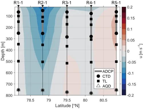
Figure 2.2: Gridded zonal velocity (m s⁻¹) section, averaged over the entire time period, with instrument locations in the water column. The grey bars mark the Acoustic Doppler Current Profilers (ADCPs), the black dots the CTDs (measuring conductivity, temperature, and pressure, i.e. depth), the black squares the temperature loggers (TLs), and the grey triangles the Aquadopps (AQDs).

2.1 Data gridding

As all instruments recorded at least every hour, a low-pass filter is applied at a period of 1 h to all the time series of instruments that recorded more often (i.e.

the temperature loggers that recorded every 30 seconds, and the Aquadopps that recorded every 20 minutes). This is done by applying a 4th order Butterworth filter to the time series with linear interpolation through gaps before the filtering and removal of those gaps afterwards, if the gap duration significantly exceeded the lowpass filter period. Afterwards hourly values of the filtered time series are used so that all time series contain data points of the same frequency.

The data are interpolated with a minimum curvature gridding method with an added tension parameter (Smith and Wessel,1990). The tension parameter is chosen to be 5 (with 0 = Laplacian interpolation, which gives a tent pole-like behaviour around data points, and ∞ = spline interpolation, which gives a smoother field, but the possibility of spurious peaks or valleys). This achieves a grid that is closest to the actual measurements, as evaluated by visual inspection. A search radius of±20 grid

(29)

2.2. HANDLING OF MISSING DATA

points is applied, as this yields a smooth grid even in depths of low data coverage.

The data are interpolated onto a grid with a temporal grid size of 1 h (i.e. the time step of the filtered measurements) and a vertical grid size of 20 m. The grid extends over a time period from 10 August 2016 to 19 July 2018 (as this is the period covered by all instruments; date of last mooring deployment to first mooring recovery) and over a depth from 40 m (20 m for velocity measurements) to 1100 m. This way no measurements are excluded. Technically the instruments furthest down in the water column only had a target depth of 750 to 780 m, but the moorings were at times subjected to strong motion and measurements acquired during those times are included in the interpolation. For analysis, the gridded data below 800 m is then removed. To achieve a coherent grid, the grid points at 20 m depth are added as NaNs for temperature, salinity, and potential density.

2.2 Handling of missing data

Except for a few single missing measurements, the CTDs only malfunctioned on three main occasions. At R3-1 the CTD at ∼265 m depth measured unexpected temperature values after 01 May 2017, likely because something was stuck in the CTD pump. This was corrected with an offset at first, but further evaluation led to the decision to disregard all temperature (and hence salinity) measurements after 01 May 2017 for this instrument. The CTD at ∼760 m depth at the same mooring recorded a peculiar rise and then offset in conductivity (and thus salinity) after 24 April 2017, which is consequently also disregarded. At R4-1 the CTD at ∼265 m depth stopped recording altogether after 31 July 2017 due to an empty battery, meaning there are no temperature, conductivity, or pressure measurements of this instrument available after this date.

(a) R3-1

27.6

27.8

28

28 28.2

34.7 34.8 34.9 35 35.1 35.2

Salinity [psu]

0 1 2 3 4 5

Pot. temperature [°C]

CTD at ~250 m CTD at ~750 m Linear regression

(b) R4-1

27.6

27.8

28

28 28.2

34.7 34.8 34.9 35 35.1 35.2

Salinity [psu]

0 1 2 3 4 5

Pot. temperature [°C]

CTD at ~250 m Linear regression

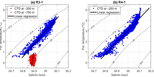
Figure 2.3: ΘS plot with linear regression of potential temperature (^◦C) and salinity (psu) of (a) the CTD measurements at∼250 m (blue dots), and at∼750 m (red dots) separately at R3-1, and of (b) the CTD measurements at∼250 m (blue dots) at R4-1.

Missing temperature and pressure measurements are replaced with nearby ADCP measurements. The difference between temperature measurements of ADCP and CTD at R3-1 is on average 0.02^◦C with a standard deviation of 0.14^◦C, and at

(30)

2.3. CALCULATIONS

R4-1 on average 0.03^◦C with a standard deviation of 0.61^◦C, which is deemed suf- ficient. Missing salinity measurements are calculated from temperature measurements, where the relationship between the two is determined by a linear regression with the data that is available at the instrument (Figures 2.3a,b). The residuals of the linear regression are randomly distributed (not shown) and this method is thus suitable in this context.

The ADCPs measured velocity profiles with 70 bins, of which approximately 8%

are lost towards the surface, which translates roughly to the upper 20 m. At R2-1 and R3-1, three respectively four entire bins are removed, due to instruments or buoyancy floats at the corresponding depths, which have zero velocity relative to the ADCP and dominate the Doppler shift of the return signal for those bins instead of scatter from the water column. Other than that some data points are excluded randomly (1.84%, 7.75%, 7.13% 1.96%, and 1.01% at R1-1, R2-1, R3-1, R4-1, and R5-1, respectively).

The temperature loggers recorded without any issues and no data are excluded.

2.3 Calculations

Different variables are derived from the gridded data and are calculated as follows:

2.3.1 Potential temperature Θ

Potential temperature is calculated with the SeaWater library of EOS-80 from the gridded salinity, temperature, and pressure, with a reference pressure of 0. Using temperature instead of potential temperature results in a small error that is naturally largest at the deepest point of the grid (i.e. at 800 m, about 0.036^◦C).

2.3.2 Buoyancy frequency N

²

Buoyancy frequency squared is calculated from potential density ρ profiles with a centred difference for each vertical grid point j, with vertical grid spacing ∆z = 20 m andj = 1 at 20 m. Gravity g is calculated from the latitude of each mooring.

N(j)² =− g

ρ(j) · ρ(j−1)−ρ(j+ 1)

2∆z . (2.1)

This means losing one value at the top and the bottom of the grid, so a NaN is added for each to achieve a coherent grid. The centred difference (evaluated over 2∆z) also adds a small smoothing compared to forward or backward differences, which are evaluated over ∆z. Gridded buoyancy frequency displays some negative values, but logarithmic probability density functions reveal them few and smaller in magnitude than the positive values. It is thus feasible to set all negative values to the smallest positive value calculated at each mooring to be able to apply a logarithmic scale.

2.3.3 Eddy kinetic energy (EKE)

Eddy kinetic energy is calculated from the deviation from the mean of zonal velocity u and meridional velocityv for each grid point as follows:

(31)

2.4. SEASONAL CYCLE

EKE = 1

2 ·(u⁰²+v⁰²). (2.2)

To evaluate mesoscale variability in particular, the velocity data are bandpass filtered between 2 and 30 days (as done in von Appen et al., 2016), and the filtered u, v are the u⁰, v⁰ that are applied in Equation 2.2. The short period limit avoids tides and inertial oscillations and the long period limit removes the seasonal cycle and interannual variations.

2.4 Seasonal cycle

The seasonal cycle of each variable is determined by first calculating monthly averages, i.e. averaging over all measurements from each of the 24 months of measurements (August 2016 to July 2018). This is done for each of the 5 moorings and each of the 40 depth levels individually. For the seasonal cycle of the full vertical length of the grid, the monthly averages are then averaged over the 40 depth levels.

Lastly, since there are two years of measurements available, the seasonal cycle is extracted by averaging over two of the same months. This means, the months July and August are slightly biased towards the year 2017, as the measurements only start in the middle of August 2016 and end in the middle of July 2018.

The seasonal cycle of the standard deviation of potential temperature, salinity, and potential density is determined by averaging the data over depth first, as the standard deviation would otherwise mainly reflect the variability in the water column, which is mostly larger than the variability in time. Then we proceed by calculating monthly standard deviations, and then averaging over two of the same months.

2.5 Water mass definitions

Water mass definitions for PW, AW, and AAW follow Rudels et al. (2005), while DW is simply defined as all water higher in density than AW and AAW. This is similar to water mass definitions in publications regarding the recirculation (e.g.

Marnela et al., 2013; Wekerle et al., 2017; Richter et al., 2018).

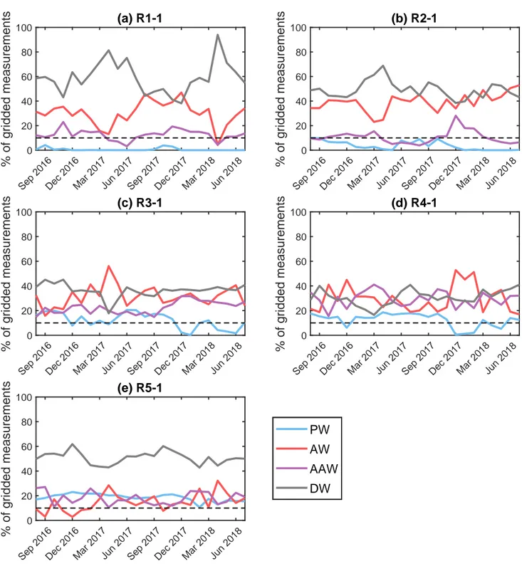
The seasonal cycle of parts of the water column that fall into a specific water mass definition is plotted by calculating the seasonal cycle only from measurements that fall into said definition, and only if the water mass makes up at least 10% of the measurements during a month, both in time and in the vertical. 10% can thus mean, the water mass occupied 10% of the upper 800 m (i.e. 80 m) all the time, or all of the upper 800 m during 10% of the time, or anything in between. This avoids averages being calculated from very little data. Nonetheless the averages are often biased towards one year, as the amount of measurements that fall into one definition in a month varies from one year to another (Figure 2.4). To calculate the seasonal cycle, the average of two of the same months is taken — if only one of the months surpasses the 10% mark, neither of the months is considered.