D I S S E R T A T I O N
zur Erlangung des akademischen Grades doctor rerum naturalium
(Dr. rer. nat.) im Fach Physik eingereicht an der
Mathematisch-Naturwissenschaftlichen Fakult¨at I Humboldt-Universit¨at zu Berlin
von
Herrn Dipl.-Phys. Peter Sinjukow geboren am 04.08.1974 in Karl-Marx-Stadt
Pr¨asident der Humboldt-Universit¨at zu Berlin:
Prof. Dr. J¨ urgen Mlynek
Dekan der Mathematisch-Naturwissenschaftlichen Fakult¨at I:
Prof. Thomas Buckhout, PhD Gutachter:
1. Prof. Dr. Wolfgang Nolting 2. Prof. Dr. Robert Keiper 3. Prof. Dr. Wladyslaw Borgiel
eingereicht am: 20. August 2004
Tag der m¨ undlichen Pr¨ ufung: 7. Dezember 2004
In this thesis a model is formulated for Eu-rich EuO. It consists in an ex- tension of the Kondo lattice model (KLM). For the KLM only a few exact statements exist. To those we add a new one, namely the exact mapping of the periodic Anderson model on the antiferromagnetic KLM for arbitrary coupling constant J.
Pure EuO is a ferromagnetic semiconductor. Eu-rich EuO exhibits a huge metal–insulator transition near the Curie temperature with a jump in resistivity of up to 13 orders of magnitude. It is the biggest jump in resistivity ever observed in nature. We theoretically reproduce this jump with the Kubo formula. We achieve very good fits already within a not fully self-consistent theory where the magnetization of the Eu spins is taken from a Brillouin function. In a fully self-consistent theory we determine the magnetization, the Curie temperature, the resistivity and other transport properties.
We calculate quantities like the electronic thermal conductivity and the thermopower, for which there are less experimental data to compare with.
Nevertheless, e.g. the calculations for the thermal conductivity seem reliable since the Wiedemann-Franz ratio with the electrical conductivity gives a reasonable result.
The conduction-electron number of Eu-rich EuO comes out of the theory independently of the conductivity. So we can calculate from the conductivity and the conduction-electron number the average Drude mobility (or scatter- ing time). This quantitiy has a jump near the Curie temperature of up to two orders of magnitude for higher impurity (oxygen vacancy) concentrations in agreement with the experiment.
Keywords:
EuO, metal-insulator transition, Kubo formula, Kondo lattice model
Zusammenfassung
In dieser Arbeit wird ein Modell f¨ur das Eu-reiche EuO formuliert. Es besteht in einer Erweiterung des Kondo-Gitter-Modells (KGM). F¨ur das KGM exi- stieren nur einige exakte Aussagen. In dieser Arbeit kommt eine neue hinzu, n¨amlich die exakte Abbildung des periodischen Anderson-Modells auf das antiferromagnetische KGM f¨ur beliebige Kopplungsst¨arkeJ.
Reines EuO ist ein ferromagnetischer Halbleiter. Eu-reiches EuO zeigt einen gewaltigen Metall-Isolator- ¨Ubergang in der N¨ahe der Curie-Temperatur mit einem Sprung im Widerstand von bis zu 13 Gr¨oßenordnungen. Das ist der gr¨oßte Sprung im Widerstand, der jemals in der Natur beobachtet wur- de. Wir reproduzieren diesen Sprung theoretisch mit der Kubo-Formel. Wir erzielen sehr gute Fits bereits in einer nicht vollst¨andig selbstkonsistenten Theorie, bei der die Magnetisierung der Eu-Spins einer Brillouin-Funktion entnommen ist. In einer vollst¨andig selbstkonsistenten Theorie bestimmen wir die Magnetisierung, die Curie-Temperatur, den spezifischen Widerstand und andere Transporteigenschaften.
Wir berechnen Gr¨oßen wie die elektronische W¨armeleitf¨ahigkeit und die Thermokraft, f¨ur die weniger experimentelle Daten zum Vergleich vorhanden sind. Nichtsdestoweniger erscheinen z.B. die Rechnungen f¨ur die thermische Leitf¨ahigkeit vertrauensw¨urdig, da das Wiedemann-Franz-Verh¨altnis mit der elektrischen Leitf¨ahigkeit einen vern¨unftigen Wert liefert.
Die Leitungselektronenzahl des Eu-reichen EuO kommt aus der Theo- rie unabh¨angig von der Leitf¨ahigkeit heraus. Daher k¨onnen wir aus der Leitf¨ahigkeit und der Leitungselektronenzahl die durchschnittliche Drude- Mobilit¨at (oder Streuzeit) berechnen. Diese Gr¨oße hat f¨ur h¨ohere Impurity- (Sauerstoff-Leerstellen)-Konzentrationen einen Sprung in der N¨ahe der Curie-Temperatur von bis zu zwei Gr¨oßenordnungen in ¨Ubereinstimmung mit dem Experiment.
Schlagw¨orter:
EuO, Metall-Isolator- ¨Ubergang, Kubo-Formel, Kondo-Gitter-Modell
1 Introduction 1 2 Motivation and applications of the Kondo lattice model 7 3 Exact results on the Kondo lattice model 11
3.1 Known exact results on the Kondo lattice model . . . 11
3.2 Exact mapping of the periodic Anderson model on the Kondo lattice model . . . 15
3.2.1 Introductory remarks . . . 15
3.2.2 Proof of exact mapping of the PAM in the extended Kondo limit on the KLM forS= 12 . . . 18
3.2.3 Proof of exact mapping of a degenerate PAM with spin constraint on the KLM forS≥1 . . . 23
3.2.4 Proof of the large Fermi volume in theS= 12 KLM for a nonmagnetic Fermi-liquid state . . . 28
4 Extension of the KLM to a realistic model describing Eu-rich EuO 33 4.1 Realistic model parameters . . . 35
5 Current density operator and transport formulae of the model for Eu-rich EuO 39 6 Solution and results of the model with external parameter hSzi 49 6.1 Solution of the model with external parameter hSzi . . . 49
6.1.1 Self-energies . . . 49
6.1.2 Coherent-potential approximation . . . 51
6.1.3 Green’s functions . . . 52
6.2 Technical details of the calculations . . . 54
6.3 Results and discussion . . . 56 iii
iv CONTENTS
6.3.1 Fit of resistivity . . . 56
6.3.2 Densities of states and mechanism of the metal- insulator transition . . . 58
6.3.3 Low-temperature minimum in the resistivity of high- resistivity samples . . . 59
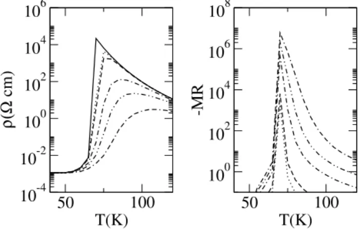
6.3.4 Resistivity in a magnetic field and magnetoresistance . 61 7 Fully self-consistent solution and results of the model 63 7.1 Fully self-consistent solution of the model . . . 63
7.2 Results and discussion . . . 66
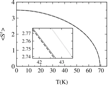
7.2.1 Magnetization and Curie temperature . . . 66
7.2.2 Comparison of theoretical and experimental resistivity 71 7.2.3 Electrical resistivity and chemical potential . . . 72
7.2.4 Electronic thermal conductivity . . . 74
7.2.5 Wiedemann-Franz ratio . . . 75
7.2.6 Seebeck coefficient and figure of merit . . . 76
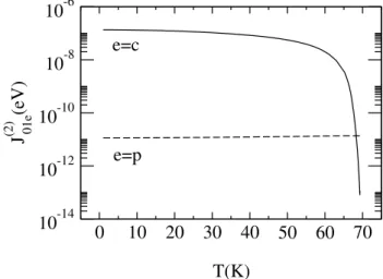
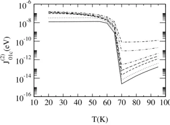
7.2.7 Conduction electron number and scattering time . . . . 79
7.2.8 Impurity electron number . . . 82
8 Summary and outlook 85
A Calculations for the proof of the large Fermi volume 89 B Calculation of the commutators for the current density op-
erator 93
C Vanishing of the u-v term in the partial integration of
Eq. (5.46) 95
D Atomic limit self-energies 99
E Modified RKKY treatment 101
Introduction
It was in 1953 when Brauer [Brauer, 1953] discovered EuO in solid so- lution with SrO [Mauger and Godart, 1986]. In 1961 Matthias et al.
[Matthias et al., 1961] identified EuO as a ferromagnetic semiconductor.
From the paramagnetic inverse susceptibility they extrapolated a Curie tem- perature of 77 K. This was 8 K too high but the exciting point experimentally and theoretically was the identification of EuO as the second truly ferromag- netic semiconductor one year after the discovery of CrBr3 by Tsubokawa [Tsubokawa, 1960, Wachter, 1979]. In the mid-fifties the possible existence of a ferromagnetic semiconductor or insulator was seriously disputed by the theoreticians. Later one recognized that only the Bloembergen-Rowland ex- change [Bloembergen and Rowland, 1955] via the polarization of the valence electrons [Wachter, 1979] could account for the ferromagnetism in insula- tors or semiconductors. In 1975 and 1976 the nearest and next-nearest neighbor exchange constants J1 and J2 for EuO were measured with neu- tron scattering by Dietrich et al. [Dietrich et al., 1975] and Passell et al.
[Passell et al., 1976], respectively. The values are J1 = (0.606±0.008)kBK andJ2 = (0.119±0.015)kBK [Wachter, 1979]. All the europium monochalco- genides, of which EuO is one member amongst EuS, EuSe and EuTe, crys- tallize in the rock salt structure where the magnetic europium ions occupy the sites of an fcc lattice. Later it was tried to calculate J1 and J2 theo- retically [Liu, 1980, Liu, 1983, Lee and Liu, 1983, Lee and Liu, 1984] using e.g. the linear combination of atomic orbitals (LCAO) method and perturba- tion theory [Lee and Liu, 1983, Lee and Liu, 1984]. At least up to that time EuO and EuS were the only known “realizations” of Heisenberg ferromagnets in nature [Lee and Liu, 1984], with a Hamiltonian given by the Heisenberg
1
2 CHAPTER 1. INTRODUCTION model
Hf f =−X
ii0
Jii0S~i·S~i0 (1.1) whereS~i is the Eu spin at siteR~i, which is of magnitudeS = 72 stemming from the 4f7 electrons, andJii0 is the exchange integral between the spins at sites R~i and R~i0. Only recently Kune˘s et al. [Kune˘s et al., 2004] calculated the indirect exchange integrals within density-functional theory using LDA+U.
For EuO with the lattice parametera= 5.1 ˚A they get their best agreement with the above cited exchange constants and with the Curie temperature of TC = 69.3 K [Wachter, 1979] for the biggest chosen value of U (= 9 eV).
If one is interested in the physics of the unoccupied conduction band of EuO, one should use the so-called s-f (or d-f) exchange model or Kondo lattice model (KLM) [Nolting et al., 1987b, Nolting et al., 1987a]. For the consideration of just one conduction band it is given by
H =X
~kσ
~kn~kσc −JX
i
S~i·~σic (1.2)
where ~k describes the conduction band, nc~kσ is the number operator for a conduction Bloch electron with wave vector ~k and spin σ, ~σic is the spin operator of the conduction electron at site R~i, and J is the constant of exchange between the conduction electron spin and the Eu spin at each site
1. Noltinget al.[Nolting et al., 1987b, Nolting et al., 1987a] used a five-band model to describe the five 5d conduction bands in EuO and for the first time combined a density-functional theory (DFT) calculation with a many-body evaluation. Schiller in his PhD thesis [Schiller, 2000] attended to the task to account for the correct symmetries of the 5d bands.
The most striking effect of the d-f exchange is the redshift of the optical absorption edge below the Curie temperature TC. It was first observed by Busch, Junod and Wachter [Busch et al., 1964, Wachter, 1979]. The corre- sponding transition is 4f75d0 → 4f65d1. Since the 4f electrons are very localized within the Eu atoms, the 4f levels are almost temperature inde- pendent. Hence, the redshift of the absorption edge is due to a redshift of the 5d conduction band. Theoretically, this is already reproduced by a simple mean-field picture of the Hamiltonian (1.2). Below the Curie temperature the conduction band is split into a spin-up and a spin-down part. With decreasing temperature the spin-up part is shifted towards lower energies
1Throughout this thesis we will useJ in energy units and all the spin operator eigen- values without the ¯h.
(redshift) by −J2hSzi whereas the spin-down-part is moved towards higher energies (blueshift) by +J2hSzi . hSzi is the magnetization of the Eu spins.
Both shifts reach their maximum of J2S at T = 0, where S = 72 is the spin quantum number of the localized Eu spins.
As an experimental matter of fact pure EuO single crystals are difficult to be fabricated. The usual method (at least in the 1970’s) was to melt Eu and Eu2O3 in a (tungsten) crucible and then to cool the crucible slowly down [Oliver et al., 1972, Schoenes and Wachter, 1974]. Depending on the ratio of Eu and Eu2O3 used, non-stoichiometric O-rich or Eu-rich EuO samples can be produced. Of exclusive interest for this dissertation is the Eu-rich EuO.
Interestingly, it has exactly the same Curie temperatureTC as the pure (sto- ichiometric) EuO [Schoenes and Wachter, 1974]. This has been used as an argument for the fact that the “lattice” of the Eu atoms is still intact in the Eu-rich samples, and that the Eu richness manifests itself in an oxygen deficiency, i.e. in oxygen vacancy sites. (Since in this thesis we are not in- terested in additional doping with e.g. Gd or La [Wachter, 1979], we will call the oxygen vacancies simply impurities.2) However, the explanation of the constancy of TC is not sufficient since each oxygen vacancy site con- tributes two electrons, which are otherwise bound in the chemical bonding with the oxygen ions. These impurity electrons, as we will show, can medi- ate an effective interaction between the Eu 4f spins. They should, therefore, in principle be responsible for a change in the Curie temperature (see also [Leroux-Hugon, 1972]). It is one of our results presented in this thesis that the effect on TC is less than 1 mK.
One of the most important physical properties of the Eu-rich EuO is a metal–insulator transition, which manifests itself in a jump in resistiv- ity near TC of up to 13 orders of magnitude under certain conditions [Torrance et al., 1972]. Over a temperature range of only several degrees Kelvin, this is the biggest jump in resistivity ever observed in nature. How- ever, the height of the jump is strongly dependent on the growing parameters (see Oliver et al. in Ref. [Oliver et al., 1972]). Starting in the 1970’s there were several theoretical attempts to describe the metal–insulator transition, some of which we will highlight in the following.
Oliver et al. were the first to propose a model for the metal–insulator transition in Eu-rich EuO [Oliver et al., 1970]. According to their first model there is a temperature-independent trap level, which stems from the oxygen vacancy sites and which crosses the redshifted conduction band at a tem- perature below the Curie temperature. The crossing means that electrons
2Eu-rich EuO will be sometimes written as EuO1−d, wheredis the “impurity” concen- tration.
4 CHAPTER 1. INTRODUCTION from the trap level can empty into the conduction band, transforming the system into a metal. Above the crossing temperature the system behaves like a doped semiconductor. The main idea of this model will also be realized within the microscopic model we will present in this thesis.
In a later paper (Ref. [Oliver et al., 1972]) Oliver et al. refer to a quan- titative fit, which was possible with a total relative band-edge-to-trap-level shift of 0.45 eV (instead of 0.26 eV in their first model). To realize such a big relative shift they assume in their second, refined model (“magnetic double donor”) two effective trap levels. The impurity electron in the first trap level has its spin more or less aligned with the spins of the Eu lattice. The second electron has the opposite spin. Therefore, there is an energy separation which becomes larger with decreasing temperature due to an increasing magnetiza- tion. BelowTC when the magnetic exchange increases, the upper trap level is shifted upwards to cross the lower conduction band edge and the lower trap level is shifted downwards. We will show that in our model such a tempera- ture dependent shift of the trap levels is unphysical. Instead there will be a shift of spectral weights. Oliver et al.’s model is sometimes called He model because in the ground state each impurity (oxygen vacancy) can absorb two electrons with opposite spin [Shapira et al., 1973, Steeneken, 2002]. Oliver et al. in Refs. [Oliver et al., 1970, Oliver et al., 1972] lead with the help of their model a more or less qualitative discussion.
Torrance et al. [Torrance et al., 1972] introduced the concept of the so- called “bound magnetic polaron”. With this they describe an electron at an oxygen vacancy which strongly interacts with the neighboring Eu spins and which is able to polarize its immediate surroundings. Therefore, in the paramagnetic phase it is rather localized giving rise to an insulating phase. In the ferromagnetic phase due to the polarization of the Eu spins the oxygen- vacancy (impurity) electron is fairly delocalized causing a metallic phase.
Also Torrance et al. in Ref. [Torrance et al., 1972] just lead a qualitative discussion.
Leroux-Hugon in Ref. [Leroux-Hugon, 1972] calculates — within the lin- ear response of the dielectric constant and the magnetic susceptibility and by the use of a variational ansatz — the transition temperature of the metal–
insulator transition for impurity concentrations of 3.5×10¹⁹to 8.3×1019cm−3, which corresponds to 0.12 % to 0.27 %. However, it is unclear why below an impurity concentration of 0.12 % there should be no metallic phase. This contradicts our theory which in principle does not have a lower bound for metallic behavior.
The first calculations of the resistivity in dependence on temper- ature we came across are the calculations by Laks and da Silva [Laks and da Silva, 1976]. They made ansatzes for the internal energy and
the entropy to get the free energy. Moreover they used the simple Drude formula for the conductivity, which is given byσ =nceµ, wherenc is the con- duction electron concentration, e the elementary charge andµ=eτ /m?e the mobility with m?e the effective electron mass and τ the scattering time. For the quasiparticle density of states they used the mean-field expression. The result is a good fit to the conductivity curve of Ref. [Torrance et al., 1972]
for temperatures below the Curie temperature but a rather bad agreement for temperatures above.
Spa leket al.[Spa lek et al., 1977] calculated the carrier concentration and the magnetic susceptibility in dependence on the temperature within a one- electron donor level model and a two-electron donor level model. However, they used mean-field for the conduction band and a magnetization-dependent shift of the one-electron donor level, which contradicts the result of the atomic limit. There is no comparison of their calculated carrier concentration with carrier concentrations from the experiment. Their inverse susceptibility be- comes zero at a temperature that is higher than the experimental Curie temperature.
Mauger [Mauger, 1983] tried to quantify the theory of the bound mag- netic polaron set out by Torrance et al.[Torrance et al., 1972]. He also used the mean-field theory for the conduction band and the simple Drude formula for the conductivity. He made special ansatzes for the free energies of the subsystems. For his fairly good fits to experimental curves he used the con- cept of compensating impurities for the conduction electrons. The fits were made to measurements of Gd doped EuO and not Eu-rich EuO. Mauger shows in Fig. 1 of his paper a phase diagram of the critical carrier density versus temperature for (Eu-rich?) EuO. It also contains a critical value of the carrier density of 0.6×1019cm−3, which corresponds to 0.02 % electron concentration per lattice site, below which there is no metallic phase. Again, this contradicts our theory, which does not have a lower bound for metallic behaviour.
Most recently Steeneken in his PhD thesis [Steeneken, 2002] calculated the resistivity in dependence on temperature for Eu-rich EuO. His concept of a temperature dependent exchange splitting of the impurity level is, how- ever, questionable since it contradicts the atomic limit result. He used the Drude formula to calculate the resistivity. He developed a theory of the de- pendence of the distribution of the impurity electron binding energies on the impurity concentration. His resistivity curves fit fairly well to the medium- resistivity samples in Ref. [Oliver et al., 1972] but rather bad to the high- resistivity samples. The inclusion of a very small concentration of acceptor sites or compensating impurities (0.001 %) changes the picture drastically.
Now with an oxygen vacancy concentration of 0.025 % he is able to repro-
6 CHAPTER 1. INTRODUCTION duce the low-temperature minimum of the high-resistivity samples of Ref.
[Oliver et al., 1972] but the high-temperature values of the resistivity are all much too high.
After all these attempts in the past to describe the behaviour of Eu- rich EuO we decided first to develop a model Hamiltonian for the system and then to solve it with the help of a Green’s function technique. We consider our model Hamiltonian a better starting point than e.g. the usage of special ansatzes for the free energy, which is always connected with some crude approximations. Furthermore we will use the Kubo formula for the case of local selfenergies to calculate the conductivity (or equivalently the resistivity). The Kubo formula, which is the correct linear response approach to the many-body problem, is supposed to be much more accurate than the simple Drude formula, where one has to make special assumptions on the mobility (or scattering time) and the effective mass of the electrons.
Moreover we will present in this thesis fully self-consistent calculations, which include the self-consistent calculation of the magnetization of the Eu spins and the Curie temperature. We will also calculate other interesting transport quantities, like the thermal conductivity of the electrons and the Seebeck coefficient.
The core of our model Hamiltonian is the famous Kondo lattice model [Eq.(1.2)], which we use to mimic the interplay between the Eu spins and the conduction band. In chapter 2 we will give a general overview of the applications of the Kondo lattice model. In chapter 3 we will first collect the exact results known so far for this model. Then we will add a new exact result for the antiferromagnetic Kondo lattice model, namely the ex- act mapping of the periodic Anderson model (PAM) on the Kondo lattice model and the consequences on the Fermi volume which follow from that.
In chapter 4 we will extend the KLM to a realistic model describing Eu-rich EuO with parameters as close as possible to the experiment. In the next chapter the current-density operator and therewith the transport formulae for the extended KLM will be derived. A not fully self-consistent solution with external parameterhSziand results thereof will be discussed in chapter 6. The fully self-consistent solution and the results following from this will be presented in chapter 7. In the last chapter a summary and conclusions will be given. In the appendices we will include some calculations which are excluded from the main text for better readability.
Motivation and applications of the Kondo lattice model
The Kondo lattice model (or s-f or s-d model) is one of the most widely used many body models in solid state physics. One of the reasons cer- tainly is its conceptual simplicity, describing an interband exchange inter- action between rather localized electrons and itinerant conduction electrons.
The ferromagnetic KLM is applied for the empty conduction electron bands of the europium chalcogenides EuX (with X = O, S, Se, Te). EuO and EuS are ferromagnetic, EuSe is an antiferromagnetic/ferrimagnetic, and EuTe is an antiferromagnetic semiconductor [Wachter, 1979]. The most prominent feature of the ferromagnetic semiconductors is the redshift of their optical absorption edge below the Curie temperature [Schoenes and Wachter, 1974].
The absorption is accompanied by the transition 4f75d0 → 4f65d1. Since the 4f states are rather localized their energies are temperature independent.
Hence, the redshift results from a down-shift of the spin-up 5d conduction band. This shift can be well understood in a mean-field picture where the conduction band is rigidly shifted proportionally to the Eu-spin magnetiza- tion hSzi by an amount ofJhSzi/2.
A second application of the KLM are the so-called local-moment metals, like Gd, Tb, Dy and Eu1−xGdxS. In contrast to the (anti)ferromagnetic semiconductors, where the magnetic order of the localized spins is due to some special kind of superexchange (Bloembergen-Rowland interaction [Bloembergen and Rowland, 1955, Liu, 1980, Liu, 1983, Lee and Liu, 1983, Lee and Liu, 1984]), in the local-moment metals an indirect coupling between the localized spins is mediated by the conduction electrons in an RKKY man- ner [Rudermann and Kittel, 1954, Kasuya, 1956, Yosida, 1957]. In the case of Gd there is at low temperatures a magnetic moment of 7.63µB. 7µB belong to the spin 72 of the 4f electrons and 0.63µB originate from the conduction
7
8 CHAPTER 2. MOTIVATION AND APPLICATIONS ...
band polarization. Hence the exchange constant J is positive (ferromag- netic).
A third group of materials for which the Kondo lattice model is appropriate are the diluted magnetic semiconductors, e.g. Ga1−xMnxAs [Matsukura et al., 1998, Dietl et al., 2001b], a group of materials which is especially promising for spintronics applications if it becomes possible to reach TC’s at or above room temperature. The diluted magnetic semicon- ductors represent dilute disordered magnetic systems with a small number of magnetic impurities and charge carriers. In the case of Ga1−xMnxAs at least the majority of Mn ions [Sanvito et al., 2001] is in the 2+ state contributing a spin of S = 5/2 and a hole in the valence band. This hole is antiferromagnetically coupled to the Mn spin [Dietl et al., 2001b, Sanvito et al., 2001, Dietl et al., 2001a, K¨onig et al., 2001]. Therefore the antiferromagnetic Kondo lattice model is appropriate here. In contrast, the conduction band is ferromagnetically coupled to the impurity spins [Sanvito et al., 2001].
The manganites (manganese oxides with perovskite structure) T1−xDxMnO3 (T = trivalent La,Pr,Nd; D = divalent Ca,Sr,Ba,Pb) show the colossal magnetoresistance [Jin et al., 1994, Ramirez, 1997]. The double-exchange mechanism, which leads to ferromagnetism above a certain critical x, was first decribed by Zener [Zener, 1951, Nolting, 1986]. He used the ferromagnetic Kondo lattice model, which for this reason was for some time also called Zener model. Due to the replacement of the trivalent by divalent ions there appears a mixture of 1 − x Mn3+ and x Mn4+ in the manganite, where the Mn4+ ions supply more or less localized spins S = 3/2 from their 3d-t2g electrons. The Mn3+ has an additional 3d-eg electron which is thought to be itinerant. However, the manganites are bad electrical conductors, because the hopping matrix element t is very small compared with the intraatomic spin-spin coupling constant J. The bandwidth W (in the simple cubic case in tight-binding approx- imation one has W = 12t) is estimated 1 – 2 eV [Satpathy et al., 1996, Pickett and Singh, 1996, Singh and Pickett, 1998], whereas J is at least 1 eV [Satpathy et al., 1996, Okimoto et al., 1995, Millis et al., 1996]. The ferromagnetic Kondo lattice model is certainly not able to describe all details of the rich phases (including phase separation [Ramirez, 1997]) of the manganites but it is looked at as a reasonable framework for gross effects in their physical behavior [Dagotto et al., 1998, Furukawa, 1994].
The so-called heavy-fermion systems form a further class of materials for which the antiferromagnetic Kondo lattice model is commonly applied apart from the periodic Anderson model. It is well known that the spin- 1/2 antiferromagnetic KLM for small J can be obtained from the PAM in
the so-called Kondo limit by the famous Schrieffer-Wolff transformation. In section 3.2 we will show that the antiferromagnetic KLM foranyfiniteJis the exact effective model of the PAM in a special “extended Kondo limit”. Heavy fermions are mainly Ce compounds. The term “heavy fermion system” comes from the fact that the effective masses of the charge carriers are enhanced by up to a factor of 1000 [Hewson, 1997]. This can be seen, for instance, by a respective enhancement of the specific heat. CeCu6−xAux is a substance where there is a change from a Kondo screened nonmagnetic state at x = 0 to a RKKY dominated state with antiferroamgnetic ordering for x ≥ 0.1 [von L¨ohneysen, 1998].
Exact results on the Kondo lattice model
3.1 Known exact results on the Kondo lattice model
Due to their non-trivial nature many-body Hamiltonians lack many exact results. In the following we will make a list of the known exact results of the Kondo lattice model (1.2).
• The “atomic limit” or zero-bandwidth limiting case (~k → T0 ∀~k) of the correlated Kondo lattice model [Nolting and Matlak, 1984, Nolting et al., 2001]:
“Correlated” means that there is an additional Hubbard term for the conduction electrons UP
inci↑nci↓. There are four temperature- independent1 quasi-particle levels in the following order (if U is large enough):
1 =T0−1
2JS , 2 =T0+ 1
2J(S+ 1), 3 =T0+U − 1
2J(S+ 1) , 4 =T0+U + 1 2JS .
The decisive point is that the spectral weights of those levels are de- pendent on the spin, the band filling and the temperature (via hSzi).
It turns out that in any case only three of the four levels have finite
1ingnoringµand its temperature dependence
11
12 CHAPTER 3. EXACT RESULTS ON THE KONDO LATTICE ...
weight. The weights are given by α1σ = 1
2S+ 1[S+ 1 +zσhSzi+ ∆−σ−(S+ 1)hnc−σi], α2σ = 1
2S+ 1[S−zσhSzi −∆−σ−Shnc−σi], α3σ = 1
2S+ 1[Shnc−σi −∆−σ], α4σ = 1
2S+ 1[∆−σ+ (S+ 1)hnc−σi],
where hSzi is the magnitization of the localized spins, hnc−σi is the average electronic occupation number at a certain site, zσ =δσ↑ −δσ↓
and ∆σ = hSσc†−σcσi+zσhSzncσi with Sσ = δσ↑S++δσ↓S−. We will make use of this limiting case when choosing the self-energy for the impurity (oxygen vacancy) electrons.
• The ferromagnetically saturated semiconductor [Shastry and Mattis, 1981, Allen and Edwards, 1982, Nolting et al., 1985, Nolting et al., 2001]:
In this limiting case all spins are aligned parallel in the z-direction.
Except for the test electron, which is put into the conduction band, the conduction band is empty. The spin-up quasi-particle band is only rigidly shifted downwards: Σc↑ = −12JS. The spin-down spectrum is more complicated [Nolting et al., 2001]:
Σc↓(E) = 1
2JS 1 + JG0(E+µ+J2S) 1− 12JG0(E+µ+ J2S)
!
(3.1) where G0(E) = N1 P
~k 1
E−~k is the local free Green’s function. If J is large enough the spin-down density of states consists of two parts.
There is spectral weight in the energy range of the spin-up density of states: this is called the scattering part because it comes from the spin flip of the spin-down electron to a spin-up electron thereby emitting a magnon and occupying a spin-up state. Secondly, there is a nar- rower so-called magnetic polaron part, which represents quasiparticles (magnetic polarons) of infinite lifetimes. They are characterized by repeated emission and absorption of magnons thereby polarizing the surroundings of the “dressed” electron.
• The second-order perturbation theory for the self-energy [Mori, 1965, Mori, 1966, Bulk and Jelitto, 1988, Bulk and Jelitto, 1990,
Nolting et al., 2001, Hickel and Nolting, 2004]:
Σ~kσc =−J
2zσhSzi{0}+J2
4 γ~kσ+O(J3) (3.2)
γ~kσ =− hSzi{0}2
G~kc{0}+ 1 N2
X
~ q
hS−~zqS~qzi{0}G~k+~{0}
qc (3.3)
+ 1 N2
X
~ q
hhS−~−σqS~qσi{0}+ 2zσhS~0znc~q+~k,−σi{0}i G~k+~{0}
qc, (3.4) where h. . .i{0} means the thermodynamic average in the interaction- free system,S~q(σ,z) is the Fourier transform of Si(σ,z), G~kc{0} = E−1
~k is the free Green’s function, and N is the number of lattice sites. Note that throughout this thesis we will leave out the ¯hfrom the definitions of the Green’s functions and spectral densities but we will leave it elsewhere to get e.g. the correct values of the transport quantities.
• The high-energy expansions of the (conduction-electron) Green’s func- tion and the self-energy [Hickel, 2004]:
The spectral density is essentially given by the imaginary part of the (conduction-electron) Green’s function G~kσc(E) =hhc~kσ;c†~kσii
A~kσ(E) =−1
πImG~kσc(E) (3.5)
The so-called spectral moments are defined by
M~kσ(n)= Z+∞
−∞
dEEnA~kσ(E). (3.6)
They can in principle be calculated by
M~kσ(n) =h[· · ·[[c~kσ,H],H],· · · ,H]
| {z } n-fold commutator
, c†~kσ]+i, (3.7)
where [. . . , . . .]+ means the anticommutator. From the spectral repre- sentation of the Green’s function one gets its high-energy expansion:
G~kσc(E) = X∞ n=0
M~kσ(n)
En+1 (3.8)
14 CHAPTER 3. EXACT RESULTS ON THE KONDO LATTICE ...
For the self-energy one can write Σc~kσ(E) =
X∞ m=0
C~kσ(m)
Em (3.9)
From the Dyson equation,EG~kσc(E) = 1 + [(~k−µ) + Σc~kσ(E)]G~kσc(E), it follows
M~kσ(0) = 1
M~kσ(1) =~k+C~kσ(0) ⇒C~kσ(0) =M~kσ(1)−~k M~kσ(2) =M~kσ(1)(C~kσ(0)+~k)+M~kσ(0)C~kσ(1) ⇒C~kσ(1) =M~kσ(2)−
M~kσ(1)2
M~kσ(3) =M~kσ(2)(C~kσ(0)+~k)+M~kσ(1)C~kσ(1)+M~kσ(0)C~kσ(2) ⇒C~kσ(2) =M~kσ(3)−2M~kσ(2)M~kσ(1) +
M~kσ(1)3
(3.10) The spectral moments can be calculated and theC-coefficients are the following:
C~kσ(0) =J
2zσhSzi (3.11)
C~kσ(1) =J2
2 ∆σ +J2
4 [S(S+ 1)−zσhSzi]−J2
4 hSzi2 (3.12) C~kσ(2) =J2
4 1 N
X
ii0
ei~k(R~i−R~i0)Tii0(hSizSiz0i+hSi−σSiσ0i)−~kJ2 4 hSzi2 +J2
4 X
i
Til
2zσhSlzc†i−σcl−σi − hSlσc†i−σclσi − hSl−σc†iσcl−σi +J2
2 X
i
Til
hSlσc†l−σciσi − hSlσc†i−σclσi
− J3
8 S(S+ 1)(1 +zσhSzi −2hnc−σi) +J3
8 zσhSzi(1 +zσhSzi)2−J3
2 zσhSzi∆σ . (3.13) We have used the Fourier transform of the dispersion ~k: Tii0 =
1 N
P
~k~kei~k(R~i−R~i0). R~l in Eq. (3.13) denotes an arbitrary site.
• The ground state of the antiferromagnetic Kondo lattice model with one conduction electron [Tsunetsugu et al., 1997]:
The ground state of the antiferromagnetic Kondo lattice model with S = 12 and one conduction electron has the total spin quantum number Stot = 12(N −1) and is unique, apart from its (2Stot+ 1)-fold spin de- generacy if the nearest-neighbor hopping-matrix element−tis negative.
(−t isThii0i for nearest-neighbor sites R~i and R~i0.)
• The ground state of the half-filled Kondo lattice model [Tsunetsugu et al., 1997]:
The ground state of the half-filled Kondo lattice model is unique and has Stot = 0 for the antiferromagnetic KLM if the lattice is bipartite, and for the ferromagnetic Kondo lattice model if the lattice is bipartite and the number of sites is equal in both sublattices.
• The “large” Fermi volume in the antiferromagnetic Kondo lattice model [Oshikawa, 2000]:
The Fermi volume of the antiferromagnetic Kondo lattice model is
“large”, i.e. contains the number of the completely localized electrons (spins), if the system is in a nonmagnetic Fermi liquid state.
To all these exact statements we add in section 3.2 the exact mapping of the periodic Anderson model on the antiferromagnetic Kondo lattice model for arbitrary coupling constantJ, first, for spinS= 12, second, for spinS = 1 and, finally, for arbitrary spin S. In subsection 3.2.4, based on the exact mapping of the PAM on the KLM, the large Fermi volume of a nonmagnetic Fermi liquid state of the antiferromagnetic KLM for S = 12 is shown.
3.2 Exact mapping of the periodic Anderson model on the Kondo lattice model
3.2.1 Introductory remarks
In section 3.2.2 it is shown that the antiferromagnetic Kondo lattice model for spin S = 1/2 and forany finite coupling constant J <0 can be obtained by an exact mapping from the periodic Anderson model in an appropriate limit, which we will call the extended Kondo limit (EKL). We thus add a rigorous statement on the Kondo lattice model to the known ones described in section 3.1. The mapping allows a direct proof of the “large” Fermi volume for a nonmagnetic Fermi-liquid state of the Kondo lattice model for S = 12 (section 3.2.4), which can replace a far more difficult topological proof by Oshikawa [Oshikawa, 2000].
16 CHAPTER 3. EXACT RESULTS ON THE KONDO LATTICE ...
As stated before, both the periodic Anderson model and the antiferro- magnetic Kondo lattice model are standard models to describe heavy fermion systems [Hewson, 1997, Fazekas, 1999, Tsunetsugu et al., 1997]. The prop- erties of those systems originate from an interplay between rather localized f electrons and itinerants,pord electrons. In the (nondegenerate) periodic Anderson model (PAM) this is mimicked in a minimal way. The Hamiltonian of the nondegenerate PAM is given by
HPAM=X
~kσ
~kn~kσc +X
iσ
fnfiσ+UX
i
nfi↑nfi↓ +X
~kiσ
(V~ke−i~k ~Ric~kσ† fiσ+ H.c.). (3.14) c(†)~kσ creates/annihilates a conduction electron (selectron) with momentum~k and spin σ. fiσ(†) is the creation/annihilation operator for an f electron at site R~i. nc~kσ and nfiσ are the respective number operators. There are nonde- generatef orbitals with energy f, with an intraorbital Coulomb interaction U and a generally ~k-dependent hybridization V~k of these orbitals with the states of the nondegenerate conduction band~k.
The Kondo lattice model is used to describe the effective physics by mod- eling the f electrons as localized quantum mechanical spins with an antifer- romagnetic spin exchange (coupling constant J < 0). The KLM is given by
HKLM =X
~kσ
~kn~kσc −X
~k~k0i
J~k0~ke−i(~k0−~k)R~iS~i·~s~k0~k . (3.15) The first part stands for the conduction band. The second part describes the interaction between localized quantum-mechanical spins S~i of magnitude S and the spins of the conduction electrons ~s~k0~k = 12 P
σ0σc†~k0
σ0~τσ0σc~kσ (with ~τ representing the Pauli matrices). J~k0~k are the (antiferromagnetic) coupling constants (J~k0~k <0).
The KLM withS = 12 represents an effective model in the so-called Kondo regime (which is relevant for the heavy-fermion systems) of the nondegen- erate PAM. There is an approximate correspondence of the two models in the Kondo regime, namely in a perturbational sense. This correspondence becomes rigorous in the Kondo limit of the PAM, which means taking the weak-coupling limit (J → 0) in the KLM. The Kondo regime of the PAM is a regime favorable for the formation of local f moments. A necessary condition for this is that the energy of the singly (doubly) occupied f or- bital lies below (above) the chemical potential: f < 0 (f +U > 0). The energy distance of the two levels f and f +U to the chemical potential
should be large compared with the hybridization so that fluctuations of the f-orbital occupancy are small. This condition is sometimes formulated in terms of the width Γ of the virtual levels of the single-impurity Anderson model [Tsunetsugu et al., 1997, Schrieffer and Wolff, 1966]:
Γ
|f|, Γ
f +U 1, (3.16)
where Γ =πρ0V2. ρ0 is the density of states of the free conduction band at the Fermi energy. V is the average hybridization (V2 = {|Vk|2}av). Via the Schrieffer-Wolff transformation, the Kondo regime of the PAM is approxi- mately mapped on the weak-coupling (small-J) regime of the Kondo lattice model. Assuming a constant free conduction-electron density of states at the Fermi energy (ρ0), the limit in which the mapping becomes exact (Kondo limit) is given by
V2 f
, V2
f +U −→0. (3.17)
The Kondo limit can be understood as
V →0 or |f|, f +U → ∞ [Lacroix and Cyrot, 1979]. (3.18) Both corresponds to J →0 on the side of the Kondo lattice model.2
This relationship between the two models is known since long ago. In 1966 Schrieffer and Wolff [Schrieffer and Wolff, 1966] showed it for the correspond- ing impurity models, the single impurity Anderson model [Anderson, 1961]
and the Kondo impurity model [Kondo, 1964]. In the single impurity An- derson model there is just one impurity f orbital at a certain site in the infinite lattice. In the Kondo impurity model there is just one f spin at a certain site in the lattice. Later the Schrieffer-Wolff transfor- mation was generalized to the periodic models, the PAM and the KLM [Lacroix and Cyrot, 1979, Proetto and Lope´z, 1981]. More recently Mat- sumoto and Ohkawa [Matsumoto and Ohkawa, 1995] claimed an equivalence between the impurity models in a special “s-d” limit, which we will call in the following “extended Kondo limit” and which differs from the con- ventional Kondo limit. Based on a dynamical mean-field theory (DMFT) argument they inferred the same equivalence to hold between the periodic
2As poined out by S. K. Kehrein and A. Mielke [Kehrein and Mielke, 1996], if f or f +U lie within the conduction band (which may be the case if just taking the limit V → 0), the Schrieffer-Wolff transformation is actually problematic because of energy denominators which become zero. The problem, however, does not occur in the extended Kondo limit.
18 CHAPTER 3. EXACT RESULTS ON THE KONDO LATTICE ...
models in the case of infinite spatial dimensions. In this section we show that via the extended Kondo limit there is a direct and rigorous mapping between the periodic models, PAM and KLM, in any dimensions. Hence, we establish a fundamental relation between both models. In contrast with the conventional Kondo limit, the equivalence in the extended Kondo limit holds forany value of the coupling constantJ <0 of the KLM.
With the fact of a rigorous mapping of the PAM on the KLM one has a general and direct answer to the long-standing question of the “correct”
Fermi surface sum rule for the Kondo lattice model. Luttinger’s theorem states that the volume enclosed by the Fermi surface (“Fermi volume”) is (a) independent of the interaction strength if no phase transitions take place and (b) otherwise only related to the total number of electrons. Luttinger’s theorem cannot be directly applied to the Kondo lattice model since, because of the localized f-spins, it is not a purely fermionic model. It is a priori unclear if the localized spins do count as “electrons” in this context. With the help of the mapping a direct and rigorous answer can be given: the respective sum rule of the periodic Anderson model is mapped on the Kondo lattice model. Therefore, we are able to prove in section 3.2.4 the “large”
Fermi volume for spin S = 12, which includes the number of localized spins in the KLM, if the system is in a nonmagnetic Fermi liquid state. We thus confirm in a much simpler way the same result of a recent topological proof by Oshikawa [Oshikawa, 2000]. Via the extended Kondo limit it will be possible to get further analytical and computational results for the Kondo lattice model. Based on the mapping every result and every analytical and computational method for the PAM can be directly applied to the KLM as long as it is compatible with the extended Kondo limit.
In subsection 3.2.2 the proof will be given for an exact mapping of the nondegenerate periodic Anderson model in the extended Kondo limit on the Kondo lattice model with S = 12. In the following subsection the proof will be extended to the S = 1-KLM and after that to arbitrary value of S. In subsection 3.2.4 we prove the large Fermi volume of the S = 12-KLM for a nonmagnetic Fermi-liquid state. All these proofs closely follow the lines of Ref. [Sinjukow and Nolting, 2002].
3.2.2 Proof of exact mapping of the PAM in the ex- tended Kondo limit on the KLM for S =
12The extended Kondo limit (EKL), Matsumoto’s and Ohkawa’s s-d limit [Matsumoto and Ohkawa, 1995], which, as we will show, leads to an exact mapping of the periodic Anderson model to the Kondo lattice model for
S = 12 for arbitrary J <0 in any dimensions, is given by f ≡ −U
2
U → ∞ , V → ∞ with V2
U →const. (3.19)
It clearly differs from the conventional Kondo limit where one has V → 0 or |f|, f +U → ∞ [Lacroix and Cyrot, 1979] [see Eq. (3.18)]. Note that in the EKL f → −∞ as U → ∞. We assume f ≡ −U2 for simplicity. It is actually only required that −2Uf → 1. Our proof of an exact mapping in the EKL consists of two basic steps. First, a finite unitary Schrieffer-Wolff transformation is performed on the Hamiltonian of the PAM. Second, the consequences of the EKL on the transformed Hamiltonian are checked. We rigorously prove that the only terms which remain relevant are those of the Kondo lattice model.
The first three terms of HPAM (3.14) are denoted by H0 =X
~kσ
~kn~kσc +X
iσ
fnfiσ+UX
i
nfi↑nfi↓ , (3.20)
the hybridization term by HV =X
~kiσ
(V~ke−i~k ~Ric~kσ† fiσ+ H.c.). (3.21)
Now we eliminate all terms which are first-order inV~k (i.e. we eliminateHV) by a unitary transformation
H¯ =eSHPAMe−S (3.22)
where the generatorS is anti-HermitianS†=−S. The condition to eliminate HV is
[S,H0] =−HV . (3.23)
The required generator turns out to be S =X
~kiσ
V~ke−i~k ~Ri
~k−f −Unfi−σc†~kσfiσ+ V~ke−i~k ~Ri
~k−f (1−nfi−σ)c~kσ† fiσ
!
−H.c.
(3.24)
20 CHAPTER 3. EXACT RESULTS ON THE KONDO LATTICE ...
The unitarily transformed Hamiltonian is given by H¯ =H0+H2+1
3[S,[S,HV]] + 1
8[S,[S,[S,HV]]] +. . . , (3.25) with
H2 ≡ 1
2[S,HV] =Hex+Hdir+Hhop+Hch , (3.26) where
Hex =−1 2
X
~k~k0i
J~k0~ke−i(~k0−~k)R~i Sif+c~k†0
↓c~k↑+Sif−c~k†0
↑c~k↓+Sif z(c~k†0
↑c~k↑−c~k†0
↓c~k↓) (3.27) Hdir =−X
~k~k0iσ
W~k0~k− 1
4J~k0~k(nfi↑ +nfi↓)
e−i(~k0−~k)R~ic~k†0
σc~kσ (3.28)
Hhop =X
~kii0σ
W~k~k −1
4J~k~k(nfi−σ+nfi0−σ)
e−i~k(R~i−R~i0)fi†0σfiσ (3.29) Hch =−1
2 X
~k~k0iσ
V~k0V~ke−i(~k0+~k)R~i
(~k0 −f −U)−1−(~k0 −f)−1
∗
∗c~k†0
−σc~kσ† fiσfi−σ + H.c. (3.30) with coupling constants
J~k0~k =−V~k0V~k∗[−(~k−f −U)−1−(~k0 −f −U)−1
+ (~k−f)−1+ (~k0−f)−1], (3.31) W~k0~k =−1
2V~k0V~k∗[(~k −f)−1+ (~k0 −f)−1]. (3.32) The spin operators in (3.27) are given byS~if = 12P
σ0σfiσ†0~τσ0σfiσ.
Now the consequences of the extended Kondo limit [Eq. (3.19)] on the transformed Hamiltonian ¯H are checked. If we assume a realistic conduc- tion band of finite width, the norm of the generator in the EKL has the asymptotics
||S||EKL∝ V
U . (3.33)
With
||HV|| ∝V and V EKL∝ √
U (3.34)
it follows that all higher commutators in (3.25), starting at the orderV3/U2, exactly vanish in the EKL,
[S,[S,HV]] , [S,[S,[S,HV]]] , . . .−→EKL 0, (3.35) and it is sufficient to consider the EKL of the remaining Hamiltonian
H¯0 ≡ H0+H2 . (3.36)
It is important to note that one cannot proceed with the original argument given by Schrieffer and Wolff for the Kondo regime of the single-impurity An- derson model [Schrieffer and Wolff, 1966]. Their argument goes as follows.
For the single-impurity Anderson model the sum overi andi0 in our expres- sion for Hhop [Eq. (3.29)] reduces to a single term for the single f orbital.
Therefore, the corresponding term for Hch [Eq. (3.30) without the sum over i] is in Schrieffer’s and Wolff’s original paper the only term which changes the number of f electrons, namely between zero and two. Hence, there the Hilbert space separates at that stage into one part of single and one part of zero and double f occupancy. The part with zero and double f occupancy becomes irrelevant at low enough temperatures or if |f|, f +U → ∞.
The reason why this argumentation is no longer valid for the periodic Anderson model is that apart from Hch [Eq. (3.30)] also Hhop [Eq. (3.29)]
changes the number off electrons at given sites. Hhop connects the subspace of single f occupancy with the subspaces of zero and double occupancy.
Therefore, the Hilbert space cannot be separated at this stage. To prove an effective fixing of the f-orbital occupation to one, which nevertheless does happen in the extended Kondo limit, one needs to apply a different and more formal line of argumentation.
We denote the s and f electron parts of H0 separately, Hs0 =X
~kσ
~kn~kσc , HU0 =X
iσ
fnfiσ+UX
i
nfi↑nfi↓ . (3.37) In the EKL the norms of the different parts of ¯H0 behave as:
||Hs0|| ∝ W = const. (3.38)
||H2|| ∝J˜≡ V2
U = const. (3.39)
||HU0|| ∝U −→ ∞EKL . (3.40) Wis the width of the free conduction band. Obviously, with respect to ¯H0the EKL is equivalent to just taking the limitU → ∞(andf ≡ −U2 → −∞). V
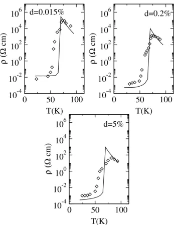
![Figure 6.4: Comparison of measured (squares, sample 34-2-30 from Ref. [Oliver et al., 1972]) and calculated resistivity (solid line) for a high-resistivity sample](https://thumb-eu.123doks.com/thumbv2/1library_info/5568292.1689742/66.892.330.625.191.420/figure-comparison-measured-squares-oliver-calculated-resistivity-resistivity.webp)