Lecture Notes in Computer Science, Vol. 9358, pp. 79–90, Springer, Berlin, 2015.
The final publication is available at link.springer.com.
Introducing Maximal Anisotropy into Second Order Coupling Models
David Hafner, Christopher Schroers, and Joachim Weickert
Mathematical Image Analysis Group, Faculty of Mathematics and Computer Science, Campus E1.7, Saarland University, 66041 Saarbr¨ucken, Germany
Abstract. On the one hand, anisotropic diffusion is a well-established concept that has improved numerous computer vision approaches by per- mitting direction-dependent smoothing. On the other hand, recent ap- plications have uncovered the importance of second order regularisation.
The goal of this work is to combine the benefits of both worlds. To this end, we propose a second order regulariser that allows to penalise both jumps and kinks in a direction-dependent way. We start with an isotropic coupling model, and systematically introduce anisotropic concepts from first order approaches. We demonstrate the benefits of our model by experiments, and apply it to improve an existing focus fusion method.
1 Introduction
Second order regularisation has become a powerful tool in a number of appli- cations. For example, it is well-suited for the estimation of depth maps, be- cause many real-world scenes are composed of piecewise planar surfaces. In a variational context, there are three popular approaches to model such a sec- ond order smoothness assumption: (i) The most intuitive one is to directly penalise second order derivatives, e.g. the Laplacian or the entries of the Hes- sian [6, 8, 16, 18, 28, 30]. However, this direct approach only allows to model dis- continuities in the second derivative that correspond to kinks in the solution.
It does not give access to the first derivative which is required to model jumps.
(ii) Thus, researchers came up with indirect higher order regularisation tech- niques; see e.g. [4, 13, 15] and related infimal convolution approaches [5]. Such indirect approaches can be interpreted in the sense of a coupling model that, in the second order case, consists of two terms: One term couples the gradient of the unknown with some auxiliary vector field, while the other one enforces smoothness of this vector field. Contrary to a direct second order penalisation, such coupling models allow to treat both jumps and kinks in the solution ex- plicitly. (iii) A related idea is to locally parameterise the unknown by an affine
function, and to optimise for the introduced parameters with a suitable smooth- ness constraint; see e.g. [21]. However, this does not allow such an explicit access to jumps and kinks [30].
Concerning first order regularisation, several approaches have demonstrated the benefits of incorporating anisotropy in the smoothness term; see e.g. [3, 12, 19, 24, 29, 34]. Thus, it seems to be a fruitful idea to also apply anisotropic concepts in second order regularisation. For instance, Lenzen et al. [16] incorpo- rate directional information into a direct second order approach. Unfortunately, as discussed, such a direct approach constrains the degree of freedom in the modelling. Also the nonlocal coupling model of Ranftl et al. [26] can be seen as related. However, in this work we aim at a fully local model that allows a natural definition of the anisotropy in terms of image and depth derivatives. In this way, we can provide a natural transition from anisotropic first to anisotropic second order approaches. In a local framework, Ranftl et al. [27] and Ferstl et al. [9]
propose a coupling model that incorporates directional image information, but the anisotropy is restricted to the coupling term. To summarise, first steps to include anisotropy into second order models have been done. However, existing approaches do not exploit successful anisotropic ideas to the full extent.
Contributions. The goal of our work is to systematically incorporate well- established anisotropic ideas from first order approaches into second order cou- pling models. We make maximal use of directional information by introducing anisotropy both into the coupling as well as into the smoothness term. In addi- tion, we propose a joint image- and depth-driven technique that allows a different amount of coupling and smoothing along and across image structures. Contrary to previous work, we apply a direction-dependent penalisation that is important for good inpainting results. Last but not least, we demonstrate the performance of our anisotropic second order technique in the context of focus fusion.
Paper Organisation. Starting with a discussion of related work, we present our variational framework for focus fusion in Section 2. In Section 3, we introduce our anisotropic second order regulariser and explain the minimisation of the full model in Section 4. We evaluate our approach and compare it to related baseline methods in Section 5. Section 6 illustrates the performance of our method on focus fusion. Finally, we summarise our work and give an outlook in Section 7.
2 Variational Model for Focus Fusion
Especially in macro photography, a typical problem is the limited depth of field of common cameras. Due to this, it is often not possible to capture a single entirely sharp image. A common remedy is to take several photographs while varying the focal plane. In this context, focus fusion describes the task of combining the acquired image stack to an all-in-focus composite that is sharp everywhere.
Most previous focus fusion approaches rely on (multi-scale) transformations of
the input images and combine them in the particular transform domain; see e.g. [1, 10, 17, 22, 25]. However, this may introduce undesirable artefacts. Inspired by [14, 20], Boshtayeva et al. [3] recently demonstrated that it is preferable to approach focus fusion by regularising the underlying depth map. Afterwards, the fusion of the focal stack images to the all-in-focus image is done in a straightfor- ward way by combining the pixels from the input images that correspond to the computed depth values. Related to this method are so-calleddepth from defocus approaches that also compute a sharp image in combination with a depth map;
see e.g. [23]. However, they are computationally more demanding and require more assumptions such as the knowledge of the point spread function of the acquisition system. Hence, we do not consider them here.
The work of Boshtayeva et al. [3] motivates us to apply focus fusion as testbed for our novel anisotropic second order regularisation technique. More specifically, we start with an initial depth mapdthat is computed in the same way as in [3]:
Based on some sharpness measure we determine the image where a pixel is in- focus. Then, we interpret the corresponding focal plane distance as depth value.
This depth mapdis equipped with a sparse confidence functionwthat indicates meaningful depth values. Next, we jointly regularise and fill-in the initial depth with the following variational approach:
E(u) = 1 2
Z
Ω
w(x)·Ψ
u(x)−d(x)2
dx + α·R(u), (1) where Ω⊂R2 describes the rectangular image domain, andαis a positive reg- ularisation parameter. Furthermore, we apply the penalisation functionΨ(s2) =
√s2+ε2withε >0 to handle outliers in the input. The regularisation termR(u) provides smooth depth maps and fills in missing information. We propose and discuss different choices of R(u) in Section 3.
3 Coupling Model for Second Order Regularisation
3.1 Isotropic Coupling Model
Compared to direct implementations of higher order regularisation, coupled for- mulations as in [4, 13] offer several advantages: First they do not require the explicit estimation and implementation of higher order derivatives. Second and even more importantly, they allow to individually model discontinuities for each derivative order. This is not possible with direct higher order models. Hence, we base our anisotropic second order regulariser on the following isotropic coupling model that replaces a direct second order smoothness term ofuby
RI(u) = inf
v
1 2
Z
Ω
Ψ |∇u−v|2
+β·Ψ |Jv|2F dx
, (2)
whereΨ(s2) =√
s2+ε2is a subquadratic function with a small positive constant ε,| · | denotes the Euclidean norm, and| · |F the Frobenius norm. Furthermore,
the vector fieldv= (v1, v2)Tcan be seen as an approximation of the gradient∇u, andJvis the Jacobian of this vector field. Since the first term in (2) inherently couples ∇u to v, we refer to it as coupling term. The second term provides smoothness of the vector fieldv. Hence, we refer to it assmoothness term. Here, the parameterβ >0 allows to steer the importance of both terms.
Let us discuss the meaning and interplay of both terms: With the nonlinear functionΨ, the smoothness term implements a first order penalisation ofvthat favours piecewise constant vector fields. For didactic reasons, let us first assume a hard coupling such that v is identical to∇u. Then, piecewise constant v are equivalent to piecewise constant first order derivatives ofu. This way, one can see that the smoothness term is responsible for modelling kinks in the solution.
With that in mind, let us now consider the behaviour of the nonlinear coupling term. With ε→0, it allows sparse deviations of the vector field v from the gradient of u, i.e. sparse peaks of the coupling term energy. Regarding v as an approximation of∇v, this shows that the coupling term allows to model peaks in the first derivative ofuwhich correspond to jumps in the solution. Summing up, the discussed coupling model provides direct access to both jumps and kinks of the unknown functionuby the coupling and smoothness term, respectively. For small ε, the coupling model in (2) resemblestotal generalised variation (TGV) of second order [4]. In many image processing and computer vision applications, such isotropic coupling models have led to high quality results. However, they do not make use of any directional information which is important for a variety of applications such as the one that we consider in this work.
3.2 Extracting Directional Information
As for instance demonstrated by Nagel and Enkelmann [19] in the context of optic flow estimation, it is highly beneficial to use the structure of a given input image to regularise the unknown flow in an anisotropic way. This allows to apply a different kind of smoothing along and across image structures. In this work, we extend this successful concept from first to second order regularisation, and in particular to the discussed coupling model. To this end, let us first determine a way to identify the structures of an image or more specifically the directions across and along them. Let f denote a given guidance image. In the case of focus fusion we take the evolving all-in-focus image as guidance. Then, we cal- culate those directionsr1andr2as the normalised eigenvectors of the structure tensor [11]
Gρ∗ ∇(Gσ∗f)∇(Gσ∗f)T
, (3)
where ∗ describes a convolution, and Gσ and Gρ are Gaussians with standard deviationσandρ, respectively. The computed eigenvectors form an orthonormal system where the vector r1, which belongs to the dominant eigenvalue, points across image structures and r2 along them.
3.3 Anisotropic Modification of Coupling Term
Let us now incorporate this directional information into the isotropic coupling model. To this end, we first consider the isotropic coupling term from (2):
CI(u,v) =Ψ |∇u−v|2
=ΨX2
`=1
eT`(∇u−v)2
, (4)
where e1= (1,0)T and e2= (0,1)T. This reformulation of the coupling term in terms of the unit vectors e1 and e2 allows to incorporate the directional in- formation as follows: First, we exchange e1 and e2 in Equation (4) with the eigenvectors r1 and r2 of the structure tensor. Second, we penalise both di- rectional components differently to introduce an anisotropic behaviour, i.e. we exchange the position of the penalisation functionΨ and the summationP2
`=1. This results in the anisotropic coupling term
CA(u,v) =
2
X
`=1
Ψ`
rT`(∇u−v)2
. (5)
Here, we apply different penalisation functionsΨ` along and across image struc- tures. This allows for instance to enforce a full coupling along edges by setting the corresponding Ψ2(s2) =s2, and to relax the coupling constraint in the or- thogonal direction withΨ1(s2) = 2ε√
s2+ε2such thatΨ10(s2) is the Charbonnier diffusivity [7]. To analyse the introduced anisotropy in a better way, let us take a look at the resulting gradient descent of (5) w.r.t.uandv:
∂tu= div D(∇u−v)
, (6)
∂tv=D(∇u−v), (7)
where div is the divergence operator, and ∂t denotes an artificial time deriva- tive to model an evolution of uand v, respectively. Equation (6) describes an evolution that occurs within gradient domain methods. However, here the tensor
D=
2
X
`=1
Ψ`0
rT`(∇u−v)2
·r`r`T (8)
steers this process in an anisotropic way. Moreover, this equation shows a nice feature of our model: When fixing the coupling variablevto0, our second order coupling model comes down to a first order anisotropic diffusion process on the unknown u; see e.g. Weickert [31] and references therein. Please note that for v=0the smoothness term vanishes since in this trivial case|Jv|2F is equal to 0.
The right hand side of Equation (7) is a reaction term that models the similarity ofvand∇u. Here, this similarity is enforced along edges (r2) while it is relaxed across them (r1). This becomes obvious by considering the tensorDin (8) that adapts the amount of similarity in a directional dependent way. This is achieved by a solution-driven scaling of the eigenvalues of D, where its eigenvectors are given byr1 andr2.
3.4 Anisotropic Modification of Smoothness Term
Let us now introduce anisotropy into the smoothness term in a similar way. To this end, we first rewrite it by means of the unit vectorse1 ande2:
SI(v) =Ψ |Jv|2F
=ΨX2
`=1 2
X
k=1
eTkJv e`2
, (9)
where the termeTkJv e`can be seen as an equivalent of the second order direc- tional derivative∂eke`u=eTkHue` with Hurepresenting the Hessian ofu. Our goal is to penalise this term differently along and across image structures. Hence, similarly to the anisotropic modification of the coupling term, we modify Equa- tion (9) by exchanginge1ande2 withr1andr2, and swapping the positions of the penalisation functionΨ and the summationP2
`=1: SA(v) =
2
X
`=1
Ψ`X2
k=1
rkTJv r`2
, (10)
where we again apply different penalisationsΨ`in both directions. Also here, let us shed light on the introduced anisotropy by analysing the associated gradient descent of (10):
∂tv=div(Jv T) = div(T∇v1) div(T∇v2)
!
, (11)
wheredivapplies the standard divergence operator div to the rows of a matrix- valued function (common definition), and thus yields a column vector with two components. Equation (11) can be seen as an anisotropic diffusion of the coupling variablev. Here the diffusion tensor
T =
2
X
`=1
Ψ`0X2
k=1
rkTJv r`2
·r`r`T (12)
describes this anisotropic behaviour: We smooth the coupling variable v differ- ently across and along image structures, where the amount of smoothness is determined by the eigenvalues ofT.
3.5 Anisotropic Coupling Model
With the proposed coupling (5) and smoothness term (10), our fully anisotropic coupled regulariser is given by
RA(u) = inf
v
1 2
Z
Ω
CA(u,v) +β·SA(v) dx
. (13)
As in the isotropic case (2), the coupling termCA(u,v) is responsible for handling jumps whereas the smoothness term SA(v) is responsible for handling kinks.
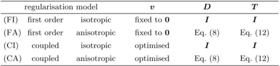
Table 1.Overview of regularisers covered by our model. Note thatDandTdegenerate to the identity matrixI ifΨ`(s2) =s2 andg`(s2) = 1,`∈ {1,2}.
regularisation model v D T
(FI) first order isotropic fixed to0 I I
(FA) first order anisotropic fixed to0 Eq. (8) Eq. (12)
(CI) coupled isotropic optimised I I
(CA) coupled anisotropic optimised Eq. (8) Eq. (12)
However, contrary to the isotropic model our new anisotropic model now effec- tively incorporates directional information to steer this coupling and smoothing.
Furthermore, for scenarios where jumps or kinks of the unknown function highly correlate with edges of the guidance image, it is beneficial to include also the strength of an image edge in addition to its direction. To this end, we scale both summands of the coupling term (5) and of the smoothness term (10) with g` (rT`∇fσ)2
, where g`(s2) is a decreasing function with g`(0) = 1, and fσ= Gσ∗f a smoothed version of the guidance imagef. This further reduces coupling and smoothing across image edges while enforcing it along them. Referring to Section 3.3 and 3.4, this solely causes an additional scaling of the eigenvalues of the tensorsDandT in Equation (8) and (12). In Table 1 we summarise different regularisation terms that result from our model with specific parameter choices.
We will evaluate those regularisers in Section 5.
4 Minimisation
Minimising the convex energy (1) with the proposed convex regularisation term comes down to solving the following system of Euler-Lagrange equations:
δuM(u)−α·div(D(∇u−v)) = 0, (14) D(v−∇u)−β·div(Jv T) =0, (15) where
δuM(u) =w(x)·Ψ0
u(x)−d(x)2
· u(x)−d(x)
(16) is the functional derivative of the data term in (1) w.r.t.u. Withnas outer nor- mal vector on the image boundary∂Ω, the corresponding boundary conditions read (∇u−v)TDn= 0 andJv T n=0.
We discretise the Euler-Lagrange equations (14) and (15) on a uniform rect- angular grid, and approximate the derivatives at intermediate grid points. Ac- cordingly, we appropriately discretise the divergence expressions with the ap- proach of Weickert et al. [33] using the parametersα= 0.4 and γ= 1. Further- more, we apply a lagged nonlinearity method where we solve the occurring linear systems of equations with a so-calledFast Jacobi solver [32].
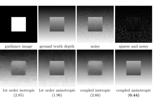
guidance image ground truth depth noisy sparse and noisy
1st order isotropic (2.85)
1st order anisotropic (1.96)
coupled isotropic (2.60)
coupled anisotropic (0.44) Fig. 1. Synthetic experiment. Top: Guidance image, ground truth depth map, noisy version, sparse and noisy version that serves as input depth map.Bottom: Computed depth maps. We state the root mean square error between the computed and the ground truth depth map in brackets under the corresponding results (×10−2).
5 Evaluation
In this section we evaluate the proposed regularisation model and compare it to the baseline methods from Table 1. To this end, we consider a synthetic data set where ground truth is available. Figure 1 (top) depicts the input guidance image, the ground truth depth map that consists of two segments with a linear slope in vertical direction, a noisy depth map, and a sparse version of it. The last one serves as input for our evaluation. More specifically, we generate the input depth map din the following way: First we add Gaussian noise of standard deviation 0.1 to the ground truth depth map, where the initial depth values range from 0 to 1. Next we randomly select 10% of this noisy version to obtain the final sparse and noisy input depth map.
Figure 1 (bottom) shows the resulting depth maps that are computed with first order isotropic(FI),first order anisotropic(FA),coupled isotropic(CI), and coupled anisotropic (CA) regularisation; cf. Table 1. For each approach the reg- ularisation parametersαandβ are optimised w.r.t. theroot mean square error (RMSE). These resulting RMSEs between the ground truth and the computed depth maps are listed right below the corresponding results in Figure 1. First, this experiment demonstrates that incorporating directional information from the guidance image is highly beneficial. Both first and coupled anisotropic regu- larisers outperform their isotropic counterparts. With anisotropic regularisation the edges of the computed depth maps are desirably sharp, while the isotropic
Table 2.Mean square error (MSE) between computed and ground truth image.
Forster et al. [10] Agarwala et al. [1] Aguet et al. [2] Boshtayeva et al. [3] our
152.12 135.97 113.73 3.47 3.08
variants cannot provide this quality. Second, the assumption of piecewise affine functions is much more suited than assuming piecewise constant depth maps in this case. Accordingly, both second order coupling models yield better results than their corresponding first order variants. It is clearly visible that the latter ones lead to piecewise constant patches, which is not desirable in the consid- ered scenario. Last but not least, the proposed coupled anisotropic regulariser provides the best results, both visually and in terms of the RMSE.
6 Application to Focus Fusion
In this section, we demonstrate the performance of our technique with the appli- cation to focus fusion. To this end, we first consider a synthetic data set from [3].
It contains a ground truth all-in-focus image that allows a comparison in terms of themean square error(MSE). Figure 2 (top left) depicts one of thirteen focal stack images and the confidence mapwfrom [3]. In Figure 2 (bottom), we com- pare the initial depth d, the result of Boshtayeva et al. [3], and our computed depth to the ground truth. We see that both approaches are able to improve the initial depth map effectively. However, our depth map shows less staircase artefacts than the first order smoothness approach of Boshtayeva et al., and is closer to the ground truth. Also our fused image resembles the ground truth all- in-focus image; cf. Figure 2 (top right). This is underlined by Table 2, where we compare our result in terms of the MSE between the fused image and its ground truth. Using the initial depth map to fuse the images gives an error of 10.55.
This is improved by [3] to obtain a MSE of 3.47. Exchanging their first order regularisation technique by our novel anisotropic second order approach yields an improvement with a MSE of 3.08. The comparison to further state-of-the-art approaches shows the usefulness of our technique for the task of focus fusion.
In Figure 3, we demonstrate the quality of our approach by an additional real-world experiment with a focus set of an insect. Since no ground truth is available, we have to restrict ourselves to a visual comparison. To this end, we depict one unsharp input image of the focal stack and the resulting fused images obtained with the approach of Boshtayeva et al. [3], and our method. Especially the zooms in thebottomillustrate that our fused image contains less errors and more small scale details than the first order approach of Boshtayeva et al. [3].
7 Conclusions
On the one hand, it is known that anisotropic techniques allow to obtain re- sults of highest quality when using first order regularisation. On the other hand,
one input image confidence map fused image ground truth image
initial depth Boshtayeva et al. [3] computed depth ground truth depth Fig. 2.Synthetic set from [3].Top: One of the thirteen unsharp input images, confi- dence map, our fused image, and ground truth image.Bottom: Rendered depth maps.
recent developments have rendered higher order regularisation very attractive.
In this paper, we build a bridge between both approaches and systematically combine such anisotropic ideas and higher order regularisation. As a result, our novel anisotropic second order regulariser allows to steer the preferred direction of jumps and kinks based on image structures. To achieve this, we have intro- duced a direction-dependent behaviour both in the coupling and the smoothness term. We have experimentally shown that this yields superior results compared to first order anisotropic and second order isotropic approaches. Moreover, we have demonstrated the usefulness of the proposed regularisation technique for the task of focus fusion. In this regard, we plan to show the benefits of our novel anisotropic second order smoothness term for further computer vision applica- tions such as stereo or optic flow computation in future work.
Acknowledgments. Our research has been partially funded by the Deutsche Forschungsgemeinschaft (DFG) through a Gottfried Wilhelm Leibniz Prize for Joachim Weickert. This is gratefully acknowledged.
References
1. Agarwala, A., Dontcheva, M., Agrawala, M., Drucker, S., Colburn, A., Curless, B., Salesin, D., Cohen, M.: Interactive digital photomontage. ACM Transactions on Graphics 23(3), 294–302 (2004)
2. Aguet, F., Van De Ville, D., Unser, M.: Model-based 2.5-D deconvolution for ex- tended depth of field in brightfield microscopy. IEEE Transactions on Image Pro- cessing 17(7), 1144–1153 (2008)
one input image Boshtayeva et al. [3] our fused image Fig. 3. Real-world focal stack of an insect consisting of thirteen images with size 1344×1201 (available at grail.cs.washington.edu/projects/photomontage).Top: One of the unsharp input images, fused image of Boshtayeva et al. [3], and our fused image.
Bottom: Zooms into the images, where red rectangles indicate obvious differences.
3. Boshtayeva, M., Hafner, D., Weickert, J.: A focus fusion framework with anisotropic depth map smoothing. Pattern Recognition 48(11), 3310–3323 (2015)
4. Bredies, K., Kunisch, K., Pock, T.: Total generalized variation. SIAM Journal on Imaging Sciences 3(3), 492–526 (Sep 2010)
5. Chambolle, A., Lions, P.L.: Image recovery via total variation minimization and related problems. Numerische Mathematik 76(2), 167–188 (Apr 1997)
6. Chan, T.F., Marquina, A., Mulet, P.: High-order total variation-based image restoration. SIAM Journal on Scientific Computing 22(2), 503–516 (2000) 7. Charbonnier, P., Blanc-F´eraud, L., Aubert, G., Barlaud, M.: Two deterministic
half-quadratic regularization algorithms for computed imaging. In: Proc. IEEE International Conference on Image Processing. vol. 2, pp. 168–172. Austin, TX (Nov 1994)
8. Didas, S., Weickert, J., Burgeth, B.: Properties of higher order nonlinear diffusion filtering. Journal of Mathematical Imaging and Vision 35(3), 208–226 (Nov 2009) 9. Ferstl, D., Reinbacher, C., Ranftl, R., R¨uther, M., Bischof, H.: Image guided depth upsampling using anisotropic total generalized variation. In: Proc. International Conference on Computer Vision. pp. 993–1000. Sydney, Australia (Dec 2013) 10. Forster, B., Van De Ville, D., Berent, J., Sage, D., Unser, M.: Complex wavelets for
extended depth-of-field: A new method for the fusion of multichannel microscopy images. Microscopy Research and Technique 65(1–2), 33–42 (Sep 2004)
11. F¨orstner, W., G¨ulch, E.: A fast operator for detection and precise location of distinct points, corners and centres of circular features. In: Proc. ISPRS Intercom- mission Conference on Fast Processing of Photogrammetric Data. pp. 281–305.
Interlaken, Switzerland (Jun 1987)
12. Hafner, D., Demetz, O., Weickert, J.: Simultaneous HDR and optic flow compu- tation. In: Proc. International Conference on Pattern Recognition. pp. 2065–2070.
Stockholm, Sweden (Aug 2014)
13. Hewer, A., Weickert, J., Scheffer, T., Seibert, H., Diebels, S.: Lagrangian strain ten- sor computation with higher order variational models. In: Burghardt, T., Damen, D., Mayol-Cuevas, W., Mirmehdi, M. (eds.) Proc. British Machine Vision Confer- ence. BMVA Press, Bristol, UK (Sep 2013)
14. Horn, B.K.P.: Focusing. Tech. Rep. Memo No. 160, MIT Artificial Intelligence Laboratory, Cambridge, MA (May 1968)
15. Horn, B.K.P.: Height and gradient from shading. International Journal of Com- puter Vision 5(1), 37–75 (Aug 1990)
16. Lenzen, F., Becker, F., Lellmann, J.: Adaptive second-order total variation: An approach aware of slope discontinuities. In: Kuijper, A., Bredies, K., Pock, T., Bischof, H. (eds.) Scale Space and Variational Methods in Computer Vision, Lec- ture Notes in Computer Science, vol. 7893, pp. 61–73. Springer, Berlin (2013) 17. Li, H., Manjunath, B., Mitra, S.: Multisensor image fusion using the wavelet trans-
form. Graphical Models and Image Processing 57(3), 235–245 (1995)
18. Lysaker, M., Lundervold, A., Tai, X.C.: Noise removal using fourth-order partial differential equation with applications to medical magnetic resonance images in space and time. IEEE Transactions on Image Processing 12(12), 1579–1590 (Dec 2003)
19. Nagel, H.H., Enkelmann, W.: An investigation of smoothness constraints for the estimation of displacement vector fields from image sequences. IEEE Transactions on Pattern Analysis and Machine Intelligence 8(5), 565–593 (1986)
20. Nayar, S.K., Nakagawa, Y.: Shape from focus. IEEE Transactions on Pattern Anal- ysis and Machine Intelligence 16(8), 824–831 (Aug 1994)
21. Nir, T., Bruckstein, A.M., Kimmel, R.: Over-parameterized variational optical flow.
International Journal of Computer Vision 76(2), 205–216 (Aug 2008)
22. Ogden, J., Adelson, E., Bergen, J., Burt, P.: Pyramid-based computer graphics.
RCA Engineer 30(5), 4–15 (1985)
23. Persch, N., Schroers, C., Setzer, S., Weickert, J.: Introducing more physics into vari- ational depth-from-defocus. In: Jiang, X., Hornegger, J., Koch, R. (eds.) Pattern Recognition, Lecture Notes in Computer Science, vol. 8753, pp. 15–27. Springer, Berlin (2014)
24. Peter, P., Weickert, J., Munk, A., Krivobokova, T., Li, H.: Justifying tensor-driven diffusion from structure-adaptive statistics of natural images. In: Tai, X.C., Bae, E., Chan, T.F., Lysaker, M. (eds.) Energy Minimization Methods in Computer Vision and Pattern Recognition, Lecture Notes in Computer Science, vol. 8932, pp. 263–277. Springer, Berlin (2015)
25. Petrovic, V., Xydeas, C.: Gradient-based multiresolution image fusion. IEEE Transactions on Image Processing 13(2), 228–237 (2004)
26. Ranftl, R., Bredies, K., Pock, T.: Non-local total generalized variation for optical flow estimation. In: Fleet, D., Pajdla, T., Schiele, B., Tuytelaars, T. (eds.) Com- puter Vision – ECCV 2014, Lecture Notes in Computer Science, vol. 8689, pp.
439–454. Springer, Berlin (2014)
27. Ranftl, R., Gehrig, S., Pock, T., Bischof, H.: Pushing the limits of stereo using variational stereo estimation. In: Proc. IEEE Intelligent Vehicles Symposium. pp.
401–407. Alcal´a de Henares, Spain (Jun 2012)
28. Scherzer, O.: Denoising with higher order derivatives of bounded variation and an application to parameter estimation. Computing 60(1), 1–27 (Mar 1998)
29. Schroers, C., Zimmer, H., Valgaerts, L., Bruhn, A., Demetz, O., Weickert, J.:
Anisotropic range image integration. In: Pinz, A., Pock, T., Bischof, H., Leberl, F. (eds.) Pattern Recognition, Lecture Notes in Computer Science, vol. 7476, pp.
73–82. Springer, Berlin (2012)
30. Trobin, W., Pock, T., D, C., Bischof, H.: An unbiased second-order prior for high- accuracy motion estimation. In: Rigoll, G. (ed.) Pattern Recognition, Lecture Notes in Computer Science, vol. 5096, pp. 396–405. Springer, Berlin (2008)
31. Weickert, J.: Anisotropic Diffusion in Image Processing. Teubner, Stuttgart (1998) 32. Weickert, J., Grewenig, S., Schroers, C., Bruhn, A.: Cyclic schemes for PDE-based image analysis. Tech. Rep. 327 (revised), Department of Mathematics, Saarland University, Saarbr¨ucken, Germany (Apr 2015)
33. Weickert, J., Welk, M., Wickert, M.: L2-stable nonstandard finite differences for anisotropic diffusion. In: Kuijper, A., Bredies, K., Pock, T., Bischof, H. (eds.) Scale- Space and Variational Methods in Computer Vision, Lecture Notes in Computer Science, vol. 7893, pp. 380–391. Springer, Berlin (Jun 2013)
34. Zimmer, H., Bruhn, A., Weickert, J.: Optic flow in harmony. International Journal of Computer Vision 93(3), 368–388 (Jul 2011)