Micro-computed tomography for natural history specimens:
a handbook of best practice protocols
Kleoniki KEKLIKOGLOU
1,*, Sarah FAULWETTER
2, Eva CHATZINIKOLAOU
3, Patricia WILS
4, Jonathan BRECKO
5, Jiří KVAČEK
6,
Brian METSCHER
7& Christos ARVANITIDIS
81,3,8
Institute of Marine Biology, Biotechnology and Aquaculture, Hellenic Centre for Marine Research,
Thalassocosmos, 71003 Heraklion, Crete, Greece.
2
University of Patras, Department of Zoology, Section of Marine Biology, 26504 Patras, Greece.
4
CNRS UMS 2700, Muséum national d’Histoire naturelle, Paris, France.
5
Scientifi c Heritage Service, Royal Belgian Institute of Natural Sciences, Vautierstraat 29, B-1000 Brussels, Belgium and Biological Collection and Data Management, Royal Museum for Central Africa, Leuvensesteenweg 13, B-3080 Tervuren, Belgium.
6
Department of Palaeontology, National Museum Prague, Václavské náměstí 68, 110 00, Praha 1, Czechia.
7
Department of Theoretical Biology, University of Vienna, Althanstrasse 14, 1090 Vienna, Austria.
*
Corresponding author: keklikoglou@hcmr.gr
2
Email: sarahfaulwetter@gmail.com
3
Email: evachatz@hcmr.gr
4
Email: patricia.wils@mnhn.fr
5
Email: jbrecko@naturalsciences.be
6
Email: jiri_kvacek@nm.cz
7
Email: brian.metscher@univie.ac.at
8
Email: arvanitidis@hcmr.gr
1
urn:lsid:zoobank.org:author:5EBBC94A-66D3-45EE-9E38-EDF7CF8B17D1
2
urn:lsid:zoobank.org:author:9BF02566-AF30-47EB-840E-DFC841B6FF84
3
urn:lsid:zoobank.org:author:BBFE2A72-6704-4446-9884-AFB1F6B09A68
4
urn:lsid:zoobank.org:author:CC392691-1414-4624-9965-867BE05CDBAF
5
urn:lsid:zoobank.org:author:7AC9797B-88EB-4844-86B9-C88DF7C06B2E
6
urn:lsid:zoobank.org:author:C2C49FC5-2D9F-4712-A029-9BF2FA9489A9
7
urn:lsid:zoobank.org:author:8777DCF2-AF42-4D51-A640-ABC1770B8572
8
urn:lsid:zoobank.org:author:737F149F-C30C-42EB-A690-5E693AD95427
Abstract. Micro-computed tomography (micro-CT or microtomography) is a non-destructive imaging technique using X-rays which allows the digitisation of an object in three dimensions. The ability of micro-CT imaging to visualise both internal and external features of an object, without destroying the specimen, makes the technique ideal for the digitisation of valuable natural history collections. This handbook serves as a comprehensive guide to laboratory micro-CT imaging of different types of natural history specimens, including zoological, botanical, palaeontological and geological samples. The basic https://doi.org/10.5852/ejt.2019.522 www.europeanjournaloftaxonomy.eu 2019 · Keklikoglou K. et al.
This work is licensed under a Creative Commons Attribution License (CC BY 4.0).
C o l l e c t i o n m a n a g e m e n t
urn:lsid:zoobank.org:pub:2B68E2FD-BE81-440B-9A02-470417CC682E
principles of the micro-CT technology are presented, as well as protocols, tips and tricks and use cases for each type of natural history specimen. Finally, data management protocols and a comprehensive list of institutions with micro-CT facilities, micro-CT manufacturers and relative software are included.
Keywords. Micro-CT, microtomography, museum specimens, 3D visualisation, virtual specimens.
Keklikoglou K., Faulwetter S., Chatzinikolaou E., Wils P., Brecko J., Kvaček J., Metscher B. & Arvanitidis C.
2019. Micro-computed tomography for natural history specimens: a handbook of best practice protocols. European
Journal of Taxonomy 522: 1–55. https://doi.org/10.5852/ejt.2019.522Table of contents
1. Scope and structure of this handbook ... 3
2. The image acquisition workfl ow ... 3
3. Protocols for micro-CT image acquisition ... 8
3.1 Pre-scan considerations and specimen preparation ... 8
3.1.1 Zoological samples ... 8
3.1.2 Botanical samples ... 10
3.1.3 Palaeontological samples ...11
3.1.4 Geological (mineral) samples ... 12
3.2 Scanning containers and scanning mediums ... 12
3.3 Scanning process ... 15
3.3.1 Calibrating the system ... 15
3.3.2 Placing the specimen ... 16
3.3.3 Setting up the detector parameters ... 16
3.4. Reconstruction ... 19
3.5 Visualisation and post-processing ... 21
3.5.1 Volume Rendering ... 22
3.5.2 Isosurface rendering ... 23
3.5.3 Segmentation ... 24
3.6 Troubleshooting ... 25
3.6.1 Beam hardening artefacts ... 25
3.6.2 Ring artefacts ... 26
3.6.3 Noise ... 27
3.6.4 Partial volume ... 27
3.6.5. Motion artefacts ... 27
3.6.6 Metal artefacts ... 28
4. Use cases ... 30
4.1 Zoological samples ... 30
4.2. Botanical samples ... 30
4.3. Palaeontological samples ... 31
4.4 Geological (mineral) samples ... 32
5. Data curation ... 33
5.1 Documentation ... 33
5.2 Data organisation, storage and archival ... 34
5.3 Data dissemination and publication ... 34
5.3.1 Data publication ... 34
5.3.2 Tools for outreach and interaction with 3D data ... 36
Acknowledgements ... 36
References ... 36
Appendix ... 47
1. Scope and s tructure of this handbook
Micro-computed tomography (micro-CT, X-ray computed tomography, high-resolution X-ray computed tomography, HRXCT/HRCT, high resolution CT, X-ray microscopy) is a non-destructive imaging technique which allows the creation of high-resolution three-dimensional data. Based on X-ray imaging, it creates a full virtual representation of both internal and external features of the scanned object. These resulting 3D models can then be either interactively manipulated on screen (rotation, zoom, virtual dissection, isolation of features or organs of interest), or an array of sophisticated 3D measurements can be performed – from simple length and volume measurements to density, porosity, thickness and other material-related parameters.
While already having been used in geology and palaeontology for decades (e.g., Carlson & Denison 1992; Simons et al. 1997; Rivers et al. 1999; Sutton et al. 2001; Carlson et al. 2003; Rossi et al. 2004;
Burrow et al. 2005; Cnudde et al. 2006; DeVore et al. 2006), in recent years micro-CT has seen a steep increase of usage in a variety of biological research fi elds such as taxonomy and systematics, evolutionary and developmental research and functional morphology (see, e.g., Faulwetter et al. 2013a and references therein).
The ability of micro-CT imaging to create accurate, virtual representations of both internal and external features of an object, at micrometer resolution, without destroying the specimen, makes the technique an interesting tool for the digitisation of valuable natural history collections. Digitisation efforts have become an important research activity of museums and herbaria, since collections represent a vast source of biodiversity information which is often underexploited due to the traditionally slow process of re-visiting physical specimens (Blagoderov et al. 2012). Digitised specimens, however, are available at the click of a mouse from any internet-enabled computer worldwide, protect the specimen from loss or damage through handling or shipping and thus have the potential to accelerate taxonomic and systematic research and allow for large-scale comparative morphological studies (Faulwetter et al. 2013a). Micro- CT imaging technology may give rise to the elaboration of ‘virtual museums’ or ‘virtual laboratories’
where digital data are shared widely and freely around the world, while the original material is stored safely (Abel et al. 2011; Keklikoglou et al. 2016). In addition, 3D models created through micro-CT scanning can be either printed or made available via interactive touch screens to be used for public display and outreach efforts.
This handbook acts as a comprehensive guide to laboratory micro-CT imaging of different types of natural history specimens, from geological and palaeontological to zoological and botanical specimens.
First, a general overview of the image acquisition workfl ow is given, presenting the basic principles of the micro-CT technology. Then, a comprehensive section on best practice protocols follows. For each of the above categories of natural history specimens, a detailed description of best practices, protocols, tips and tricks and use cases are given, from specimen preparation to fi nal use of the resulting models.
However, each specimen is different, and each study has a different scope, so naturally there is no standard protocol that can be universally applied. The information given in this handbook merely acts as a starting point. The last section of the main text comprises information on the data management of the micro-CT datasets, including best practices on metadata, storage and dissemination. Finally, an appendix includes a glossary which explains the domain-specifi c terms used throughout the text and additional useful information, such as lists of institutions with micro-CT facilities, micro-CT manufacturers and annotated list of software.
2. The image a cquisition workfl ow
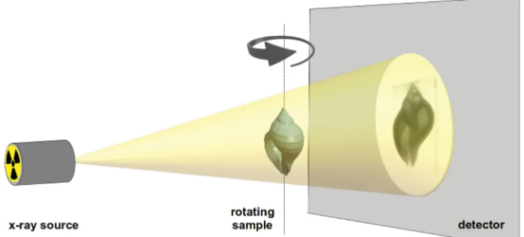
The basic principle of the micro-CT technique is related to the acquisition of a large set of radiographic
projections (2D images) of an object around a rotation axis. The rotated object is placed between an
X-ray source and an X-ray detector (Fig. 1) and the free adjustment of the source-object distance (SOD) and object-detector distance (ODD) allows greater resolution in comparison to clinical CT scanners (Schambach et al. 2010).
The micro-CT technique depends on X-rays which are high energy electromagnetic radiation ranging from hundreds of eV to hundreds of keV. X-rays photons are generated by electron beams. The X-ray source contains an X-ray generator (a vacuum tube) in which electrons are released from a fi lament (the cathode) and are highly accelerated by an electric potential difference (Fig. 2). Then, the electronic beam is focused on a metal target (the anode) and produce X-rays according to two different processes:
The electrons are decelerated by the atomic nucleus of the target and part of their kinetic energy is converted into an emitted X-ray photon. This phenomenon is called ‘braking radiation’ or Bremsstrahlung.
The output spectrum consists of a continuous spectrum of X-ray energies ranging from 0 to the voltage of the X-ray source.
Fig. 1. Schematic overview of the image acquisition process. Image by the Hellenic Centre for Marine Research (HCMR) micro-CT lab.
Fig. 2. Schematic overview of the X-Ray generator.
The electrons may collide with target orbital electrons and be ejected from the orbit. Subsequently, an electron from a higher energy level will replace the ejected electron and the energy left by this displacement will be transferred to an emitted X-ray photon. The energy of the X-ray photon (fl uorescent photon) is the difference between the two energy levels, a characteristic of the target’s material.
The appropriate choice of the target’s material aims to ensure that the energy effi ciency of the braking radiation is high (its atomic number is high) and the fusion point is high enough to endure high power. Tungsten is used as the main material for high power applications. Another typical material is molybdenum for fi ner resolution applications. Sutton et al. (2014) mention that a tungsten target source is considered ideal for palaeontological specimens and a molybdenum target source for specimens which are included in amber.
Filters (e.g., aluminium, copper, aluminium and copper combined) can be used to prevent the lowest X-ray photon’s energy reaching the specimen, thus avoiding artefacts during the reconstruction procedure (beam hardening; Section 3.6). Figure 3 shows a typical spectrum generated by an X-ray generator for 100 kV, along with the spectrum when it is fi ltered with a 0.5 mm copper plate.
X-rays are attenuated along their paths through the specimen due to three types of interactions:
photoelectric absorption, Rayleigh scattering and Compton scattering. This attenuation is characterised
Fig. 3. The spectrum generated by an X-ray generator at 100kV with and without fi ltering. Image generated by
the simulation environment https://www.oem-xray-components.siemens.com/x-ray-spectra-simulation.
by a linear coeffi cient μ (E,Z) in cm
-1that corresponds to the contribution of each type of interaction and depends on the energy of the incident beam and the atomic number of the material encountered.
The total attenuation of an incident beam passing through a well-defi ned specimen can be computed as a sum or an integration of individual attenuations. This property is a key to tomographic reconstruction, called an inverse problem, as the measurement of the total attenuations on different angles will lead to knowledge of a discrete set of attenuations (in a voxel grid) along the path through the specimen.
The X-rays photons that have been transmitted through the specimen are then collected on a detection device. A scintillator screen absorbs the X-ray beam and re-emits it in the form of light. This light may be captured by CCD or CMOS cameras, digitised by a photodiode array in a fl at-panel detector. The choice of a detector is usually a trade-off between its pixel resolution and its fi eld of view.
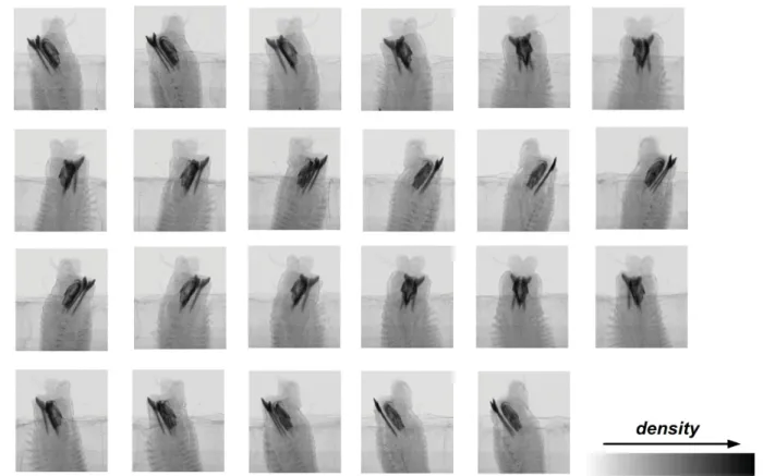
The resulting image is a radiograph (projection image) whose pixel values are the X-ray transmission as measured by the detector, usually mapped to 16-bit gray values (ranging from 0 to 65535). This type of acquisition is called absorption-contrast. When displayed as a positive image, the darkest parts of an X-ray image are the most absorbing ones and the lightest parts are those with the lowest absorption (e.g., air) (Fig. 4). The reconstructed tomographic image consists of voxels whose values correspond to the X-ray attenuation at each point in the sample.
The aforementioned projection images are reconstructed into cross-section images using specifi c reconstruction software. A reconstruction algorithm is run to get a volumetric representation of the density of the specimen, including its inner features. The most common reconstruction software use fi ltered back projection algorithms for the recovery of the attenuation maps of the radiographs.
Fig. 4. Example of the projection images resulting from the scanning process. Image by HCMR micro-
CT lab.
Specifi cally, projection images, which are taken from every angle of the sample, results in sinograms which represents the aforementioned attenuation maps (Betz et al. 2007). The cross-section images (slices) are created by these sinograms using back-fi lter algorithms. Each projection image is smeared back across the reconstructed image and creates the back-projection images which transmit the measured sinogram back into the image space along the projection paths. The back-projection image is a blurred cross-sectional image. This blurring effect can be moderated using mathematical fi lters (Sutton et al.
2014) and the algorithms that use the combination of back projection and fi ltering are known as fi ltered back-projection algorithms. The combination of the back-projection images will localise the position of the sample. As the number of projections increase, the position and shape of the object becomes more defi ned (Fig. 5).
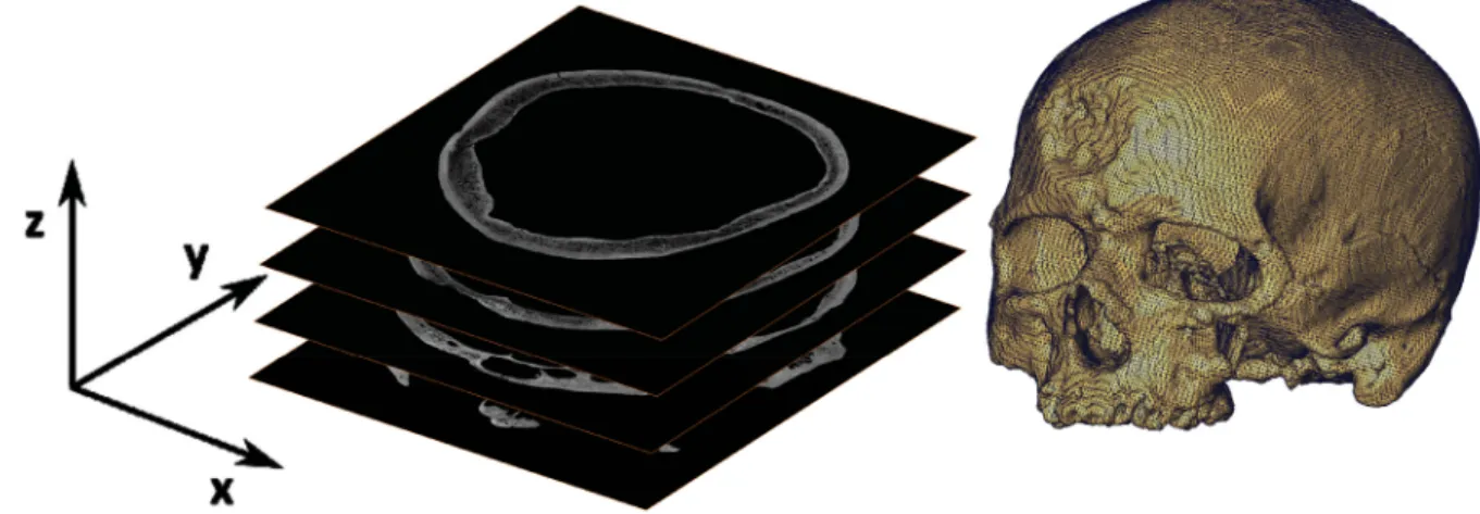
The reconstruction procedure results in a 3D image where each voxel codes the local density of the specimen. It is usually exported as a stack of 2D images in a given orientation (Fig. 6). The micro- CT dataset can then be processed with dedicated software for 3D visualisation (either through volume rendering or isosurface rendering, see Section 3.5) or further analysis (see Tables 8 and 9 for comprehensive lists of software). The rendered images can be also used for the creation of 3D videos which are an excellent tool for sharing a preview of a micro-CT dataset (Abel et al. 2012).
Fig. 5. Schematic overview of the reconstruction procedure. Image by HCMR micro-CT lab.
Fig. 6. Data processing from a stack of 2D images to a 3D model. Image by MNHN. i k i d l b
3. Protocols fo r micro-CT image acquisition
3.1. Pre-scan c onsiderations and specimen preparation
The selection of micro-CT as a technique for specimen visualisation depends on the aim of the specifi c study. The limitations of the method must be considered, e.g., colour cannot be represented and structures below a certain size cannot be detected. An additional consideration when working with museum specimens is to ensure that the museum curator will allow imaging with micro-CT (including contrast enhancement through staining, if needed).
The fi rst and major step to obtain good results is to achieve a sound contrast difference between the specimen and its surrounding medium. Contrast enhancement agents can be used to improve the quality and clarity of the scanning result: 1) when the specimen has inadequate contrast, 2) when extreme attenuation differences between soft and hard tissue need to be reduced (setting of the contrast level in the scan becomes easier), 3) to segment tissues or organs more easily, and 4) to identify specifi c target features of the specimen.
Rehydration or dehydration procedures may be needed before staining, depending on the preservation medium of the specimen, or after staining and on the medium in which the specimen will be scanned.
3.1.1. Zoologic al samples
Dense material, such as bones and other calcifi ed tissues, usually does not require any specifi c preparation. In soft tissue specimens, where visualisation can be diffi cult due to the low X-ray absorption of unmineralised tissues (Metscher 2009a; Gignac & Kley 2014), contrast enhancement agents are commonly applied.
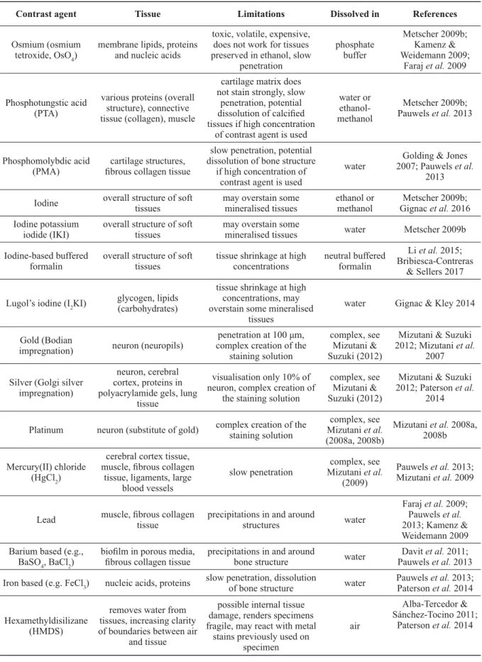
A series of the most common contrast agents used in zoological samples is presented in Table 1. In general, contrast agents with a high atomic number are more effi cient since they result in an increased X-ray absorption (Pauwels et al. 2013). However, the selection of an appropriate and effi cient contrast enhancement agent is a combination of several considerations such as the type of the target tissue (see Table 1), the medium in which the specimen was fi xed and stored (Metscher 2009a), the acidity and the penetration rate of the contrast agent (Metscher 2009b; Pauwels et al. 2013; Paterson et al. 2014), as well as the price and toxicity of the staining used. Contrast agents with low penetration rate are more effective when used in relatively small specimens with a sample size of only a few cm
3(Pauwels et al.
2013). Staining larger specimens may require longer staining time, as the penetration rate in larger samples may be slower. Contrast agents dissolved in buffered formalin could prevent potential tissue deterioration due to the long staining period for large specimens (Li et al. 2015).
Staining of fresh samples will usually give optimal results. However, the results of the staining can be infl uenced by certain treatments, such as freezing prior to fi xation and the fi xation process (Gignac et al.
2016). If possible, long-term storage in ethanol or unbuffered formalin between fi xation and staining should be avoided, as this may affect the morphology of the specimen or alter tissue characteristics which in turn affect staining properties (e.g., iodine stains bind to lipids, which can be dissolved in alcohols (Gignac et al. 2016), and unbuffered formalin or other acidic liquids may decalcify tissues).
However, this is not always possible for museum specimens, and good results have been also achieved with museum specimens stored for years and decades. These fi ner details of fi xative, storage medium, tissue characteristics and staining properties are still insuffi ciently known and will require further studies in the future.
Micro-CT scanning is a powerful visualisation method with several advantages, but might not be
appropriate for all kinds of specimens. Some contrast enhancement agents are acidic (e.g., PTA, PMA,
FeCl
3) and when used in high concentrations they may dissolve calcifi ed tissues, such as bones, and
destroy the specimen structure (Pauwels et al. 2013). Therefore, in cases where calcifi ed structures are
Contrast agent Tissue Limitations Dissolved in References Osmium (osmium
tetroxide, OsO4) membrane lipids, proteins and nucleic acids
toxic, volatile, expensive, does not work for tissues preserved in ethanol, slow
penetration
phosphate buffer
Metscher 2009b;
Kamenz &
Weidemann 2009;
Faraj et al. 2009
Phosphotungstic acid (PTA)
various proteins (overall structure), connective tissue (collagen), muscle
cartilage matrix does not stain strongly, slow
penetration, potential dissolution of calcifi ed tissues if high concentration
of contrast agent is used
water or ethanol- methanol
Metscher 2009b;
Pauwels et al. 2013
Phosphomolybdic acid
(PMA) cartilage structures, fi brous collagen tissue
slow penetration, potential dissolution of bone structure
if high concentration of contrast agent is used
water Golding & Jones 2007; Pauwels et al.
2013 Iodine overall structure of soft
tissues may overstain some
mineralised tissues ethanol or
methanol Metscher 2009b;
Gignac et al. 2016 Iodine potassium
iodide (IKI) overall structure of soft
tissues may overstain some
mineralised tissues water Metscher 2009b Iodine-based buffered
formalin overall structure of soft
tissues tissue shrinkage at high
concentrations neutral buffered formalin
Li et al. 2015;
Bribiesca-Contreras
& Sellers 2017
Lugol’s iodine (I2KI) glycogen, lipids (carbohydrates)
tissue shrinkage at high concentrations, may overstain some mineralised
tissues
water Gignac & Kley 2014
Gold (Bodian
impregnation) neuron (neuropils) penetration at 100 μm, complex creation of the
staining solution
complex, see Mizutani &
Suzuki (2012)
Mizutani & Suzuki 2012; Mizutani et al.
2007 Silver (Golgi silver
impregnation)
neuron, cerebral cortex, proteins in polyacrylamide gels, lung
tissue
visualisation only 10% of neuron, complex creation of
the staining solution
complex, see Mizutani &
Suzuki (2012)
Mizutani & Suzuki 2012; Paterson et al.
2014
Platinum neuron (substitute of gold) complex creation of the staining solution
complex, see Mizutani et al.
(2008a, 2008b)
Mizutani et al. 2008a, 2008b
Mercury(II) chloride (HgCl2)
cerebral cortex tissue, muscle, fi brous collagen
tissue, ligaments, large blood vessels
slow penetration complex, see Mizutani et al.
(2009)
Pauwels et al. 2013;
Mizutani et al. 2009
Lead muscle, fi brous collagen
tissue precipitations in and around
structures water
Faraj et al. 2009;
Pauwels et al.
2013; Kamenz &
Weidemann 2009 Barium based (e.g.,
BaSO4, BaCl2) biofi lm in porous media,
fi brous collagen tissue precipitations in and around
bone structure water Davit et al. 2011;
Pauwels et al. 2013 Iron based (e.g. FeCl3) nucleic acids, proteins slow penetration, dissolution
of bone structure water Pauwels et al. 2013;
Paterson et al. 2014
Hexamethyldisilizane (HMDS)
removes water from tissues, increasing clarity of boundaries between air
and tissue
possible internal tissue damage, renders specimens fragile, may react with metal
stains previously used on specimen
air
Alba-Tercedor &
Sánchez-Tocino 2011;
Paterson et al. 2014
Table 1 (continued on next page). Overview of the most common contrast agents for soft zoological
tissues.
included in the specimen tissue the minimum, but still effective concentration of acidic agents needs to be identifi ed prior to staining, or alternatively other non-acidic agents should be used for contrast enhancement.
Contrast agents dissolved in ethanol (e.g., PTA, iodine) may cause shrinkage when used on specimens which are not stored in ethanol. In such cases a water based contrast enhancement agent may be more appropriate and safe to use; otherwise a gradual dehydration procedure needs to be followed prior to staining. Shrinkage due to desiccation may destroy the sample and in addition it can create movement artefacts during scanning (Johnson et al. 2011). Samples can also be critical point dried, freeze-dried or chemically dried with Hexamethyldisilazane (HMDS) and then scanned without any surrounding liquid medium in order to increase the contrast between tissues. Generally, these methods can dry the samples without inducing morphological changes to the tissues, although they might render the sample fragile or cause moderate shrinkage (Faulwetter et al. 2013b; Pauwels et al. 2013; Krings et al. 2017). The drying can be performed both on stained and unstained samples, but care needs to be taken with HMDS, which may react chemically if applied in combination with certain stains (e.g., silver stains, see Paterson et al.
2014).
Specimens from museum collections usually need to remain completely intact, and thus any alterations that might be caused by the staining procedure need to be taken into account. Besides the alterations previously mentioned (decalcifi cation, shrinkage) the removal of the contrast enhancement agents after scanning is an additional important consideration before using this method on museum specimens. The stability of the stain might depend on the fi xation or preservation medium, the age of the specimen, and the type of tissue (e.g., chitin, muscles, calcifi ed tissue) (Schmidbaur et al. 2015). Iodine staining was successfully removed from insects (Alba-Tercedor 2012) and from millipedes (Akkari et al. 2015) by re-immersion into 70% ethanol, and from polychaete tissues using 96% ethanol for 48 hours, while PTA stain was removed using NaOH for 6 hours (Schmidbaur et al. 2015). However, treatment of iodine stained tissues with sodium thiosulfate and of PTA stained tissues with 0.1 M phosphate buffer (pH 8.9) destained the samples even more than their initial unstained status, thus indicating an actual alteration of the tissues characteristics (Schmidbaur et al. 2015). Gignac et al. (2016) also indicated that destaining does not really restore a specimen to its original chemical state, e.g., when iodine stained tissues are treated with sodium thiosulfate, the iodine is transformed to iodide, which is colorless and remains in the tissues.
3.1.2. Botanical samples
Micro-CT scanning of botanical specimens is usually restricted to non-pressed specimens, i.e., those that possess a certain three-dimensional structure. Technically, pressed herbarium specimens can also
Contrast agent Tissue Limitations Dissolved in References
Zinc chloride (ZnCl2) muscle, fi brous collagen
tissue slow penetration water Pauwels et al. 2013
Ammonium molybdate tetrahydrate
(NH4)2MoO4
muscle, fi brous collagen
tissue slow penetration water Pauwels et al. 2013
Sodium tungstate (Na2WO4)
muscle, fi brous collagen
tissue unknown water Pauwels et al. 2013;
Kim et al. 2015 Gallocyanin-
chromalum nucleic acids low overall contrast water
Presnell &
Schreibman 1997;
Metscher 2009b
Table 1 (continued).
be scanned under certain circumstances, but the results will likely be of limited research value. Suitable botanical specimens include soft tissues (e.g., fl owers, leaves, buds, fruits) and hard tissues (e.g., stems, twigs, roots, nuts). Generally, ligneous hard tissues are more easy to scan than soft tissues, as they do not dry out easily and provide a good contrast due to the higher density of their secondary cell walls.
Plant tissues can often be scanned without any need for fi xing, preservation of sample, or application of contrast agents. Fruits, nuts, thick roots and wooden structures and even fl owers, if provided with a liquid environment around the stem (van der Niet et al. 2010) can often simply be scanned fresh without any further preparation. However, if a high resolution of these tissues is required, smaller pieces may be cut from the original sample to decrease the camera-sample distance. Such smaller samples dry out faster and thus may require additional means to prevent dehydration such as wrapping in plastic or Parafi lm
®, scanning in a sealed container, or coating the specimen with additional materials (e.g., Korte & Porembski 2011).
Soft tissues are often transparent to X-rays and may require the use of contrast agents, as well as additional preparation to prevent shrinkage during scanning due to desiccation (Stuppy et al. 2003;
Leroux et al. 2009). If the sample needs to be fi xed and/or stained, a variety of solutions are available.
Common fi xatives for botanical samples are FAA (formalin–acetic acid–alcohol), formaldehyde, or ethanol (e.g., Leroux et al. 2009; Staedler et al. 2013). However, ethanol has been shown to induce shrinkage in plant tissues and might not be appropriate for all types of studies, e.g., vascular cylinders might be compressed or ruptured if ethanol is used (Leroux et al. 2009).
Samples fi xed in a liquid substance will usually require being scanned in a liquid environment as well, either fully submerged or sealed in a small chamber to prevent drying out. Alternatively, samples can be embedded in agarose or paraplast, but as this will introduce noise and reduce contrast these media are only recommended for samples that are either naturally dense or have been treated with heavy-metal stains (see Table 2).
Table 2 (continued on next page). Overview of the most common contrast agents (heavy metals) for soft botanical tissues.
Contrast agents Effects and limitations References
Uranyl acetate toxic, only slight increase of contrast values compared to other stains
Leroux et al. 2009;
Staedler et al. 2013
Iodine no noticeable contrast increase
Korte & Porembski 2011; Staedler et al.
2013 Potassium
permanganate
permanganate caused visible damage to samples as soon as after 2d infi ltration (Fig. 5F), and infi ltration for 8 days usually resulted in total sample loss; occasionally increased the contrast of only a part
of the sample, leaving other parts unchanged
Staedler et al. 2013
Lugol’s solution causes visible sample damage after several weeks of infi ltration Staedler et al. 2013 Phosphotungstate
(PTA)
highest contrast increase on the more cytoplasm- and protein-rich
tissues (ovules, ovary wall and pollen) Staedler et al. 2013
Lead citrate
work best on vacuolated tissues (petals, sepals and fi laments);
highest contrast increase on the more cytoplasm- and protein-rich tissues (ovules, ovary wall and pollen); precipitates in presence of carbon dioxide in the form of lead carbonate crystals [38] that
accumulate on the surface of the sample
Staedler et al. 2013
Bismuth tartrate
work best on vacuolated tissues (petals, sepals and fi laments);
highest contrast increase on the more cytoplasm- and protein-rich tissues (ovules, ovary wall and pollen); rendered the samples very
delicate and easy to damage
Staedler et al. 2013
A variety of contrast enhancing heavy metal stains has been tested on plant tissues, to varying levels of success and with different tissue specifi cities. A thorough comparative study has been performed by Staedler et al. (2013). Table 2 summarises the application areas and effects of various heavy metal stains.
3 .1.3. Palaeontological samples
Palaeontological specimens (i.e., fossils) may need to be isolated from rock matrices before scanning in cases where the specimen and the matrix show a similar X-ray absorption. Fossils can be extracted from their matrix mechanically by washing, wet sieving and the use of several tools such as needles, knives and chisels (Green 2001; Sutton 2008) or chemically, depending on the chemical composition of the surrounding matrix. For example, fossils embedded in calcareous rocks can be isolated using sulphuric acid (Vodrážka 2009), phosphatic fossils can be extracted using acetic acid (Jeppsson et al. 1999) and plant mesofossils in clay or mud stones can be extracted in water with sodium carbonate, potassium hydroxide or hydrogen peroxide (Wellman & Axe 1999). The maceration procedures of palaeontological specimens usually involve physical breakdown, removal of calcareous material, removal of siliceous material, removal of other inorganic material, oxidation, sieving, cleaning and concentrating the organic rich residue (Green 2001). A detailed manual for extraction techniques in palaeontology can be found in Green (2001). However, potential damage of the specimen using chemical extraction methods must be considered (Sutton 2008). If there is no possibility of extraction of the fossil and the contrast between the specimen and the matrix is too low, a synchrotron phase-contrast imaging may be a better solution for the visualisation of such specimens (Sutton et al. 2014). Specimens in amber can be scanned directly without any particular preparation.
3.1 .4. Geological (mineral) samples
Strictly speaking, the only preparation that is absolutely necessary for scanning geological specimens is to ensure that the object fi ts inside the fi eld of view and that it does not move during the scan (Ketcham &
Carlson 2001). Since the full scan fi eld is a cylinder, it is suggested to scan an object of cylindrical geometry, either by using a coring drill to obtain a cylindrical sample of the geological material being scanned, or by packing the object in a cylindrical container with either X-ray-transparent fi ller or with material of similar density (Ketcham & Carlson 2001).
For some applications the sample can also be treated to enhance the contrast between the different structures. Examples include injecting soils and reservoir rocks with NaI-laced fl uids to reveal fl uid-fl ow characteristics (Wellington & Vinegar 1987), injecting sandstones with Woods metal to map out the fi ne- scale permeability, immersion in caesium chloride to visualise connected porosity of crystalline rocks (Kuva et al. 2018) and soaking samples in water to emphasize areas of differing permeability, which can help to reveal fossils (Zinsmeister & De Nooyer 1996).
3.2 . Scanning containers and scanning mediums
At the end of the staining procedure, the sample is removed from the solution and washed in distilled water or ethanol (depending on the contrast agent solvent). However, Staedler et al. (2018) immediately fi xed the plant specimens with 1% PTA in formalin–acetic acid–alcohol (PTA/FAA) without washing
Contrast agents Effects and limitations References
Osmium tetroxide
work best on vacuolated tissues (petals, sepals and fi laments);
highest contrast increase on the more cytoplasm- and protein-rich tissues (ovules, ovary wall and pollen); poor penetration for en-bloc
infi ltration → best on open and thin material (open buds, tissues only a few cells thick)
Staedler et al. 2013
Iron diamine samples could not be detected (no increase in contrast) Staedler et al. 2013
Table 2 (continued).
the samples with ethanol. If specimens are stained or naturally dense they can be scanned in liquid or gel media (e.g., water, ethanol, agarose). If they are to be scanned in air, excess fl uid should be blotted away in order to prevent motion artefacts during scanning due to the accumulation of fl uid on the bottom of the container (Gignac et al. 2016). Then, the specimen is placed in a sample holder and stabilised in a vertical position for the scanning procedure. The choice of the appropriate sample holder depends on the sample size, the morphology of the specimen and the material of the sample holder.
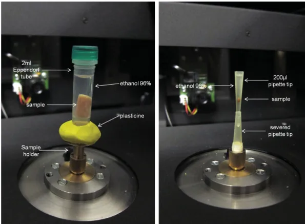
Micro-CT companies usually provide a range of several sample holders to the users. It is essential that specimens do not move, settle or wobble during scanning; even a small shift can ruin the image data and necessitate a re-scan (Sutton et al. 2014). Nevertheless, users often create new sample holders according to their needs in order to prevent movement of the specimen during scanning. Glass containers are rarely used since they have a high X-ray absorption; however, glass presents a higher contrast with the background compared to the plastic container, therefore allowing more accurate delineation of the region of interest which corresponds to the inner part of the container (Paquit et al. 2011). Materials such as polypropylene, styrofoam and fl orist foam have low X-ray absorption, making them ideal as sample holders. It is also quite common to use pins and clips in order to stabilise the specimen; however, care must be taken in order not to damage museum samples. Sealable plastic bags from which air has been pressed out can be used to prevent drying of specimens (Gignac et al. 2016). Small specimens can be placed in test tubes, aliquot tubes, plastic straws or micropipette tips (200, 1000, 5000 μL) (Metscher 2011; Alba-Tercedor 2012; Staedler et al. 2013; Gignac et al. 2016) (Figs 7, 8B–D). The bottom end of pipette tips can be cut off in order to drag down the samples and to stabilise them by entering a preparation needle (Staedler et al. 2018). Paraffi n wax can be used in the lower end of the pipette tip as a seal and to stabilise the sample, while Parafi lm
®can be used to seal the upper end of the tip (Staedler et al. 2013; Fig 8C). The lower end of pipette tips can also be heat-sealed if they need to be fi lled with a liquid medium surrounding the specimen. Batch scanning can help to scan large numbers of small samples at the same time and thus decrease overall scanning time: individual samples mounted in pipette
Fig. 7. Setup of scanning containers. Images by HCMR micro-CT lab.
tips can be mounted in a 1 ml syringe tube and stabilised with resin or epoxy glue (Staedler et al. 2013, 2018; Fig. 8).
Specimens can be submerged in fl uid (e.g., formalin, ethanol or water) during scanning to prevent desiccation (Gignac et al. 2016). Ethanol is less dense than water and provides greater tissue contrast in comparison to water (Metscher 2009a). Scanning small specimens within a liquid medium prevents them from getting stuck on the container’s walls. Care must be taken to remove bubbles from the liquid medium in the sample holder as they can create a blurring effect (Metscher 2009a). Agarose can also be used as a scanning medium for small specimens (Metscher 2011). The use of air as a scanning medium gives excellent results for unstained or dried specimens or for studying the internal structure of specimens. However, scanning in air is not recommended when studying the external morphology of specimens previously immersed in liquid, since the small amount of liquid that will remain on the external surface will be visible as an additional layer in the reconstruction images (Fig. 9).
Fig. 8. Sample mounting techniques for plant specimens of different sizes. A. Large samples (>10 mm).
B–D. Medium-sized samples (1–10 mm). E–F. Small samples (<1 mm). Image from Staedler et al.
2013, reproduced under a CC-BY license.
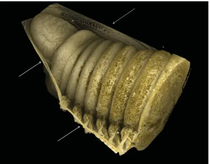
Fig. 9. External morphology of the polychaete Lumbrineris latreilli Audouin & Milne Edwards, 1834.
Specimen had been preserved in ethanol and was subsequently blotted dry on a tissue and scanned in air.
The remaining ethanol (shown by arrows) can be observed clinging to the anterior end of the polychaete.
Image by HCMR micro-CT lab, CC-BY Sarah Faulwetter.
Large plant samples (>10 mm) can be mounted in acrylic foam and scanned in a solvent atmosphere, whereas medium-sized plant samples are best scanned immersed in the solvent (Staedler et al. 2013;
Fig. 8A–B). Red and brown algae are easily scanned after having being dried in air. Scanning of the more fi lamentous green algae and seagrasses within a liquid medium creates artefacts, because their leaves have a low X-ray absorption. Personal experiments showed that staining with PTA or iodine could not improve the resolution. Chemical drying of fi lamentous algae (e.g., HMDS) and scanning in air can have satisfactory results, but due to shrinkage this method is not suggested when aiming to study the internal leaf structure.
Palaeontological specimens are usually scanned in air. However, a celluloid fi lm in organic water-soluble glue is suitable as a scanning medium for isolated microfossils (Görög et al. 2012). Isolated specimens can be also fi xed on plastic holders by nail polish (or any other reversible fi xing matter). For combined SEM and micro-CT studies SEM holders can be used. However, fi xation of fossils must be on a thick layer of nail polish to avoid contact or close placement of the observed fossil and the metallic holder, which can occlude the view of the sample. Larger specimens are fi xed in specially prepared holders made of plastic or polystyrene. The main concern is to prevent potential movements of the fossil during the radiography process. Sutton et al. (2014) mentioned that different X-ray penetration between the different axes of a palaeontological sample could cause noise and artefacts and they suggest to bury the specimens in a substance such as fl our for low density samples and sand for more dense samples.
3.3. Sca nning process
Scanning settings differ in terms of voltage, exposure time, magnifi cation and resolution depending on the scope of study, the material of the specimen, the specimen size and the instrument used. A careful balance between all the scanning parameters is necessary to ensure an ideal result and a best practice protocol.
3.3.1. C alibrating the system
In order to achieve micrometer precision, the incident beam needs to be thin, focused and stable during the acquisition. This calibration of the source includes a software-driven warm-up and focusing. Depending on the scanning system, the user should set the main parameters, including the metal of the source target (if the instrument has this option), the amount of fi ltration, the source intensity (in mA) and the source voltage (in kV). The source voltage should be set up in a way that the beam will have suffi cient energy to penetrate the specimen and reach the detector. Furthermore, the source intensity should not be too high as the detector may be saturated. On a projection image, the dynamic range (max-min gray value) has to be maximised. A good contrast on the set of projections leads to a good contrast on the fi nal CT image.
Too much transmission will reduce the contrast between different densities, while a low transmission will increase the noise level in the images. The contrast should be checked over a complete rotation of the specimen. Adjustment of fi lter and voltage settings should aim at a minimum transmission between 10 and 50%.
Scanning of unstained soft tissues usually does not require the use of fi lters, as they are characterised by a high X-ray transmission. An exception could be a sample which is characterised by a combination of soft and dense structures (e.g., a vertebrate organism), where the use of a fi lter may be helpful.
Dense structures, such as bones, shells and other calcifi ed structures, are characterised by a high X-ray
absorption, as they contain elements with high atomic number (Schambach et al. 2010). Such structures
appear dark on the images and they have low X-ray transmission, so the use of fi lters during scanning
is necessary. These fi lters can be made of aluminium, copper or a combination of the two. Filters reduce
artefacts caused from beam hardening effects (Meganck et al. 2009; Abel et al. 2012), while the spread
of the X-ray energy distribution is reduced (see Section 3.6). However, the use of fi lters shifts the
grayscale values downwards, resulting in less contrast between tissues (Meganck et al. 2009). Contrast
between tissues can be achieved by decreasing the voltage and in addition, the use fi lters in cases of
dense structures is recommended for artefact reduction.
3.3.2. P lacing the specimen
The specimen is placed on a rotating platform between the X-ray source and the detector. It has to be centred vertically and horizontally along the detector. A high-precision rotating mount may help to centre small specimens. When acquiring a specifi c region of interest, this region has to be centred instead of the whole specimen. The specimen must not touch either the source or the detector at any time during a complete rotation.
The magnifi cation depends on the distance between the source, the specimen and the detector. The fi nal image voxel size V results from the equation V = p × ss/sd , where p is the detector pixel size, ss the source to specimen distance and sd the source to detector distance. The distances ss and sd may be automatically set by the system or may need a calibration. When the positions of the detector and the rotating platform are set, the calibration usually consists in acquiring a set of radiographs of a calibration object placed on the rotating platform. A greater magnifi cation and resolution could decrease beam-hardening effects (see Chapter 3.6), but will increase scanning duration. A big specimen size can prevent achieving high magnifi cation and resolution while a smaller fi eld of view is required for the identifi cation of the smallest structures (Dixon et al. 2018). For this reason, micro-CT datasets acquired at different resolutions can be combined in order to provide more information (Dixon et al. 2018 and examples therein).
3.3.3. S etting up the detector parameters
The calibration of the detector is software-driven (but may need regular initiation by the user) and includes the acquisition of two types of images:
the dark fi eld image is the resulting image when no X-radiation is emitted. This signal comes from the dark current in the photodiodes of the detector. This image is an offset that will be subtracted from every radiograph.
the open fi eld images are the response of the detector pixels to the incident beam when no specimen is placed in the system. The software may require a couple of images at different beam intensities or only one for the maximum beam intensity.
In case some pixels are defective, their response will strongly differ from that of their neighbouring ones. When they are detected, a defective map is built and these pixels are ignored during an acquisition.
Their values are replaced by an interpolation of the values of non defective neighbouring pixels. The defect map should be computed once a month.
Several parameters can usually be changed to infl uence the imaging process; however, not all scanner models offer the same options. A few important parameters are listed below.
The exposure time E relies on the same principle as the photographic exposure time. It controls the amount of time (in seconds) during which the X-rays will be captured. The detector should collect enough photons at each angle to ensure a good contrast on the radiograph. The effective dynamic range of the image is proportional to the exposure time if it is not saturated, and hence the short exposure results in the low signal-to-noise ratio. High density or thick specimens (e.g., fossils) will need a longer exposure time because fewer photons will be transmitted through them. However, excessively high exposure times may saturate the detector panel (i.e., raise brightness above its maximum measurable threshold). The scanning duration is obviously longer when the exposure times are longer. The use of higher voltage can result in a decrease of the exposure time.
A way to ensure a suffi cient contrast without ending up with long scans is to use a binning parameter.
Instead of having single cells (or pixels) collecting X-rays on the detector, the signal is acquired using
‘bins’ of 4 adjacent pixels (for a 2×2 binning). The X-ray fl ux per (binned) pixel is four times higher and
the exposure time can be reduced accordingly. The pixel size and the resulting voxel size are twice as
large in linear dimension (and the resulting volume image is ⅛ as large). Binned acquisition results in a well-contrasted fast scan, but at the price of lower resolution.
An averaging parameter A (frame averaging) may be set to improve the image quality. A set of images will be acquired for every angle and only the mean image will be recorded. A higher number of frames increases the signal-to-noise ratio. Therefore, it is usually recommended to increase the frame averaging for high dense samples when the signal-to-noise ratio is too low.
Depending on the detector employed, a pausing parameter P can be used to prevent an afterimage effect.
The detector photodiodes need a few ms to get cleared of the image. If the acquisition is too fast, residual information from the previous image can appear on the next image. The pausing parameter therefore helps to fully discard the signal from the previous image. It also ensures that the specimen is perfectly still after the rotation.
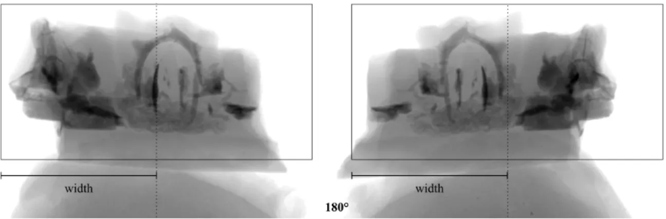
The number N of radiographic images needed to perform a reconstruction can be estimated by measuring the maximum width W of the projected specimen on a radiograph (in pixels) using the formula N = π × W (for a 360° scan; Fig. 10). Note that to determine the maximum width the specimen should be rotated, as irregularly shaped specimens may have different widths at different angles. Acquiring less than N projection images will provide an incomplete dataset for the reconstruction algorithm. The reconstruction will be still possible, but its quality will be degraded.
The total scanning time T (in seconds) can be computed with the following formula: T = N × (P + (E × A)).
Other scanning settings include the selection of the rotation step, random movement and 180/360° scan.
The selection of an increased rotation step is useful when the scanning duration needs to be reduced but it can result in images of reduced quality and increased noise. Random movement can be activated to reduce ring artefacts, but should not be used when the position of the samples is not secured or when the pixel sizes are very small. The full 360° rotation is selected for scans where the sample consists of a combination of high dense materials inside low dense materials and helps to avoid depletion artefacts.
The half (180°) rotation can be used when is it necessary to reduce the scanning time. The simultaneous scan of multiple samples (batch scan) can be used to reduce the overall scanning duration. A short scan duration is benefi cial when specimens are scanned in air and therefore dehydration and shrinkage need to be avoided.
Fig. 10. Measuring the maximum width W (in pixels) of the projected specimen (as the distance from
the rotation axis - dotted line - to the farthest end of the sample) to calculate the number of radiographs
needed. This measurement is done for the angular position of the rotating platform where the projected
specimen is the widest. For a complete rotation, the projected specimen would stay within the limits of
the rectangle. Photo by MNHN.
Examples regarding the scanning parameters of zoological, botanical, geological and palaeontological samples are included in Tables 3–6.
Specimen Voltage (kV)
Current
(μΑ) Filter System Source Reference
Alligator mississippiensis
(vertebrate) 150–200 130–145 copper GE phoenix
v|tome|x s240 molybdenum Gignac & Kley 2014 Dromaius novaehollandiae
(vertebrate) 130–180 145–190 copper GE phoenix
v|tome|x s240 molybdenum Gignac & Kley 2014 Polychaeta (invertebrates) 60 167 none SkyScan 1172 tungsten Faulwetter et al. 2013a
Apporectodea caliginosa Apporectodea trapezoides (anterior part – invertebrates)
65–70 100 none Skyscan 1173 tungsten Fernández et al. 2014 Ommatoiulus avatar
(invertebrate) 60 67 none Zeiss/Xradia
MicroXCT-200 tungsten Akkari et al. 2015 Snake embryos (vertebrates) 40 100 none Zeiss/Xradia
MicroXCT-200 tungsten van Soldt et al. 2015
Table 3. Examples of scanning parameters for zoological samples.
Specimen Voltage (kV)
Current
(μΑ) Filter System Source Reference
root samples of
Asplenium theciferum 50 unknown none
in-house nano-CT at University of
Ghent
unknown Leroux et al. 2009
Xylem of Laurus 50 275 none Nanotom 180 XS;
GE unknown Cochard et al. 2015
macadamia nuts-in-shell 60 unknown unknown SkyScan 1172 tungsten Plougonven et al.
2012 Flower of Bulbophyllum
bicoloratum 50 100 unknown Xradia Micro-
XCT-200 tungsten Gamisch et al. 2013
Table 4. Examples of scanning parameters for botanical samples.
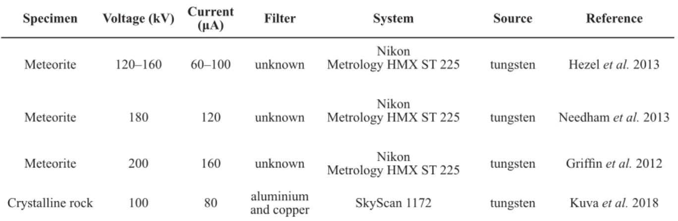
Specimen Voltage (kV) Current (μA) Filter System Source Reference
Meteorite 120–160 60–100 unknown Nikon
Metrology HMX ST 225 tungsten Hezel et al. 2013
Meteorite 180 120 unknown Nikon
Metrology HMX ST 225 tungsten Needham et al. 2013
Meteorite 200 160 unknown Nikon
Metrology HMX ST 225 tungsten Griffi n et al. 2012
Crystalline rock 100 80 aluminium
and copper SkyScan 1172 tungsten Kuva et al. 2018
Table 5. Examples of scanning parameters for geological samples.
3.4. Rec onstruction
The reconstruction workfl ow varies among the different scanning systems as each system usually has its own software and most reconstruction steps are automated (Sutton et al. 2014). However, the setting of some reconstruction parameters is necessary and depends on the scope of the reconstruction and the scanning quality. Concerning the scanning quality, misalignment during the acquisition, noise and ring artefacts may be corrected or improved by using the appropriate reconstruction parameters.
Prior to the reconstruction procedure, some systems can check the projection images for potential movements during the scanning procedure. The alignment of the projection images may fi x these movements. If sample movements cannot be corrected through the reconstruction procedure, the scanning process should be repeated.
Following the alignment of the projection images, the reconstruction software creates a histogram with the frequency the grayscale values representing the density distribution of the micro-CT dataset. The specifi c range of the histogram values can display different parts of the organisms (Fig. 11). Generally, the peaks in the histogram values represent different structures concerning the different densities. Dense structures such as bones and shells are represented by higher grayscale values compared to soft tissues.
The user can choose to restrict the range of values, to suppress or include specifi c densities, in order to emphasize different structures in the reconstruction of the sample. The range of the grayscale values can also be taken into consideration in order to avoid noise and to isolate unwanted structures (e.g., sample holder).
During the reconstruction procedure, the reconstruction can be restricted to a specifi c area of the specimen by creating a region of interest (ROI). For example, the reconstruction of the jaws of a polychaete can be achieved by the creation of a ROI which comprises only these target structures (Fig. 12). This method
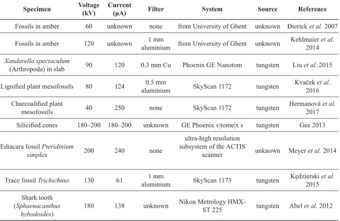
Specimen Voltage (kV)
Current
(μΑ) Filter System Source Reference
Fossils in amber 60 unknown none from University of Ghent unknown Dierick et al. 2007 Fossils in amber 120 unknown 1 mm
aluminium from University of Ghent unknown Kehlmaier et al.
2014 Xandarella spectaculum
(Arthropoda) in slab 90 120 0.3 mm Cu Phoenix GE Nanotom tungsten Liu et al. 2015 Lignifi ed plant mesofossils 80 124 0.5 mm
aluminium SkyScan 1172 tungsten Kvaček et al.
2016 Charcoalifi ed plant
mesofossils 40 250 none SkyScan 1172 tungsten Hermanová et al.
2017 Silicifi ed cones 180–200 180–200 unknown GE Phoenix v|tome|x s tungsten Gee 2013 Ediacara fossil Pteridinium
simplex 200 240 none
ultra-high resolution subsystem of the ACTIS
scanner unknown Meyer et al. 2014
Trace fossil Trichichnus 130 61 1 mm
aluminium SkyScan 1173 tungsten Kędzierski et al.
2015 Shark tooth
(Sphaenacanthus hybodoides)
180 138 unknown Nikon Metrology HMX-
ST 225 tungsten Abel et al. 2012
Table 6. Examples of scanning parameters for palaeontological samples.
can minimise the time of the reconstruction procedure and the size of the reconstructed dataset. The reconstruction duration also depends on the computational resources and capacities, the size of the dataset and the algorithm used (Sutton et al. 2014).
Fig. 11. Histogram of the grayscale value frequency of the scanned specimen (bivalve Musculus costulatus (Risso, 1826). Each peak represents a different structure (in terms of density) of the scanned bivalve. Bright grayscale values (representing low densities) are located at the left side of the histogram, darker values (representing high values) at the right side of the histogram. A. The selection of a range including all peaks, reveals the more detailed morphology of the bivalve (both soft/low density and hard/high density structures). B. A restricted range of histogram values removes structures with brighter values (= low densities). C. A restricted range of histogram values including only one peak reveals only the darkest values (= most dense structures) of the bivalve which correspond to the shell. Image by HCMR micro-CT lab.
Fig. 12. Cross-section image without (A) and with (B) a selection of a region of interest (red square) for
the reconstruction of polychaete jaws. Image by HCMR micro-CT lab.
Reconstructed data should ideally be saved without any compression or down-sampling (i.e., as 16 bit TIFF fi les). However, these fi les are large, so if storage space is an issue or data are to be shared, the creation of compressed image formats (e.g., 8 bit PNG, JPG) can be considered – but always taking into account the detail of information required for the planned analyses. The best lossless image format is TIFF as it can also store metadata (e.g., voxel size, specimen info, scan parameters); however, different systems offer different options.
3.5. Vi sualisation and post-processing
The reconstructed images can be visualized in 3D using volume rendering software. A variety of products are available (see Table 7). The creation of interactive 3D volumes allows the users to explore the dataset from any direction and to manipulate its appearance by changing the rendering parameters (Ruthensteiner et al. 2010). The 3D visualisation of specimens may be used for taxonomic purposes, as specifi c structures can be visualised in their original orientation and shape (see Faulwetter et al. 2013a).
A volume can be visualised through volume rendering or through extracting an isosurface (Sutton et al.
2014). Details related to these visualisation methods are presented below.
Table 7 (continued on next page). 3D Volume Rendering software (modifi ed table from Walter et al.
2010 and Abel et al. 2012).
Software Licence
Type URL
Amira commercial www.amira.com
Arivis (web-based
software) commercial http://vision.arivis.com/
BioImageXD free http://www.bioimagexd.net
Blender free www.blender.org
Brain Maps (web-based
software) free http://brainmaps.org
CTVox free https://www.bruker.com/products/microtomography/micro-ct-software/3dsuite.html
Dragonfl y
free licences available for researchers
with non- commercial
activities/
commercial
http://www.theobjects.com/dragonfl y/
DRISHTI free http://sf.anu.edu.au/Vizlab/drishti/
Fiji (Is Just
ImageJ) free http://fi ji.sc/
Huygens commercial http://www.svi.nl
ImageJ free https://imagej.nih.gov/ij/
Image-Pro commercial http://www.mediacy.com
Imaris commercial http://www.bitplane.com/
The post-processing of micro-CT datasets can include simple analyses (e.g., density estimation through the calculation of the grayscale values, porosity, thickness) or advanced morphometric analysis (e.g., geometric morphometrics). The latter requires segmentation of the image (isolation of features of interest and creation of a geometric surface model – see below).
3.5.1. Volume Rendering
The volume rendering procedure assigns colour and opacity to each voxel according to the grayscale values of the sample (Kniss et al. 2002). Some ranges of the histogram can be set to be transparent, mostly to exclude the voxels of the surrounding medium or container. Whenever a structure can be well-defi ned by its density/grey level on an histogram, it is easily isolated on a volume rendering image by setting everything else transparent (Fig. 13). Advanced rendering parameters give the user the opportunity to apply artifi cial colours and brightness in order to create a realistic/useful rendering.
Fig. 13. Volume rendering of a specimen where the gray level coding for (A) air and (B) air+soft tissues are transparent. Histograms of the grayscale values are included for both images where the selected threshold is indicated by the blue line and the opacity curve is indicated by the red line. Image by MNHN.
Software Licence
Type URL
Mimics commercial www.materialise.com/mimics
Octopus commercial https://octopusimaging.eu/
Open
Inventor commercial http://www.openinventor.com/
Simpleware commercial www.simpleware.com
Slice:Drop (web-based
software) free http://slicedrop.com/
SPIERS free https://spiers-software.org/
tomviz free http://www.tomviz.org/
VG Studio
Max commercial www.volumegraphics.com
Volocity commercial http://www.improvision.com
VolViewer free http://cmpdartsvr3.cmp.uea.ac.uk/wiki/BanghamLab/index.php/VolViewer
VTK free http://www.vtk.org/
Table 7 (continued).
3.5.2. Isosurface rendering
An isosurface is a geometric mesh connecting 3D points of a constant intensity within a volume (Fig. 14). The thresholding procedure (or binarisation) of the slices, where the grayscale images are transformed to black and white images, is important for the creation of the 3D model while all voxels are connected above the thresholding value (for software options see Table 8). The 3D model construction is based on the marching cubes algorithm (Lorensen & Cline 1987). The calculation might be time- consuming, depending on the size of the data and the computer capacities. The resulting triangle-mesh can be visualised and it is suitable for analysis (e.g., shape analysis, volume, geometric morphometrics, or fi nite-element modelling). For software packages related to 3D analysis see Table 9.
Software Licence Type URL
Amira commercial www.amira.com
BioImageXD free http://www.bioimagexd.net
Dragonfl y free licences available for researchers with non-
commercial activities/
Commercial
http://www.theobjects.com/dragonfl y/
DRISHTI free http://sf.anu.edu.au/Vizlab/drishti/
ilasti free http://ilastik.org/
Mimics commercial www.materialise.com/mimics
Octopus commercial https://octopusimaging.eu/
Simpleware commercial www.simpleware.com
SPIERS free https://spiers-software.org/
VG Studio Max commercial www.volumegraphics.com
Table 8. Segmentation software (modifi ed table from Walter et al. 2010 and Abel et al. 2012).
Fig. 14. A marine worm (Polychaeta, Phyllodocidae, Phyllodoce). A. Photograph (CC-BY-SA Hans
Hillewaert). B. Volume rendering. C. Isosurface rendering. Images B and C by the HCMR micro-CT lab.
3.5.3. Segmentation
The main drawbacks of volume rendering and isosurface rendering are that neighbouring structures cannot be discerned if their densities are too homogeneous and their borders not contrasted enough. In these cases it is diffi cult to discern a specifi c structure among voxels of similar grey value (for example:
visualising specifi c organs within the body where all organs are of similar densities). Segmentation is the process of selecting (‘labelling’) voxels of interest in order to visualise them separately of the whole dataset (or to generate a 3D model of these user-defi ned structures) (Fig. 15). The segmentation procedure Table 9. 2D/3D analysis software (modifi ed table from Walter et al. 2010 and Abel et al. 2012).
Software Licence Type URL