Costs and Benefits of Electric Vehicles and District Cooling Systems: A case study in Singapore

Research Collection

Report

Costs and Benefits of Electric Vehicles and District Cooling Systems: A case study in Singapore

Author(s):

Borzino, Natalia; Fonseca, Jimeno A.; Riegelbauer, Emanuel; Nevat, Ido; Schubert, Renate Publication Date:

2020-12-07 Permanent Link:

https://doi.org/10.3929/ethz-b-000454933

Rights / License:

In Copyright - Non-Commercial Use Permitted

DELIVERABLE TECHNICAL REPORT

Version 07/12/2020

D2.3. – COSTS AND BENEFITS OF ELECTRIC VEHICLES AND DISTRICT COOLING SYSTEMS: A CASE STUDY IN

SINGAPORE

Project ID NRF2019VSG-UCD-001

Project Title Cooling Singapore 1.5:

Virtual Singapore Urban Climate Design

Deliverable ID D2.3. – Cost-Benefit Assessment

Authors Natalia Borzino; Jimeno Fonseca; Emanuel

Riegelbauer; Ido Nevat and Renate Schubert.

DOI (ETH Collection)

Date of Report 07/12/2020

Version Date Modifications Reviewed by

1 30/11/2020 Renate Schubert

2 30/11/2020 Ido Nevat

1 Abstract

Urban heat brings negative consequences for communities, their people and their assets. Different strategies and measures could be introduced to reduce urban heat and increase Outdoor Thermal Comfort (OTC). However, these strategies and measures, not only brings with diverse levels of benefits, but also result in differing costs. Typically, a Cost-Benefit Analysis (CBA) is used to assess the cost and benefits of policy interventions. Yet, there are situations in which it is difficult to measure the benefits of a heat reducing measure in monetary terms, making a CBA difficult to implement. In such cases, a Cost-Effectiveness Analysis (CEA) could be applied as an alternative method. In this study, we implement a CEA to assess the effects of two urban heat mitigation strategies related to new technologies: a district cooling system on the one side and the electrification of the vehicle fleet on the other side. We perform our assessment in a study site located in the City Business District (CBD) area in Singapore. We evaluate the costs and the effects of the two technologies applied to the study area.

Hereby, the main benefit we are interested in is OTC, but also in final energy consumption and greenhouse gas emissions. In this study, we use the Physiological Equivalent Temperatures (PET) as a proxy measure for OTC (i.e. the lower, the better). We compare different implementation scenarios for both technologies, with different degrees of the technologies’ applications (i.e. 33%, 66%, 100%).

We also assess the Business-As-Usual (BAU) scenarios, i.e. the scenarios without any additional implementation of the new technologies. Our results suggest that, on the one hand, the implementation of 100% District Cooling Systems presents the highest net-benefits compared with the BAU scenario.

In fact, this scenario presents the highest PET improvement (-1.1

C) at rather low costs (- 10.78%) compared to the BAU. Furthermore, this scenario brings the highest additional positive effects on energy consumption and greenhouse gas emissions. On the other hand, a 100% electrification of buses only presents the highest net-benefits as it brings an improvement in PET (-0.71

C) at only a 0.6%

increase of the costs compared with BAU. However, the 100% electrification of the vehicle fleet presents

the highest PET reduction (i.e. -0.91

C) as well as highest reductions in energy consumption and

greenhouse gas emissions across all scenarios, yet at the highest additional costs (i.e. +11.48%)

compared with the BAU. In addition to these results, policymakers might consider people’s level of

acceptance and support for the implementation of specific urban heat mitigation measures. This aspect

could be studied by means of Willingness-to-Pay elicitation. Overall, our study gives valuable insights

into the costs and benefits of the implementation of new technologies for heat mitigation purposes in

Singapore.

Table of Content

1 Abstract ... 2

2 Introduction ... 4

3 Study area description, mitigation strategies and scenarios ... 5

3.1 Study area ... 5

3.2 Mitigation strategies and scenarios ... 6

4 Methods ... 7

4.1 General scope of our analysis ... 7

4.2 The Cost-Effectiveness Ratio CER ... 8

4.3 Estimation of Costs ... 10

4.4 Estimation of Benefits ... 12

4.5 Using CER for decision purposes ... 13

5 Results ... 15

5.1 Electric Vehicles ... 15

5.2 District Cooling Systems ... 21

6 Conclusions ... 29

6.1 Summary and assessment of findings ... 29

6.2 Limitations and next steps ... 31

7 References ... 32

8 Appendix ... 35

2 Introduction

Hot and humid weather results in a wide range of negative consequences for communities, their people and their assets. Economy, health, well-being, human behaviour, infrastructures and the natural environment are all affected by very high daily temperatures and by humid weather conditions. Urban warming and Urban Heat Island (UHI) tend to yield an exacerbation of these effects. Any degree by which we can lower the temperature comes along with additional costs but also benefits. The higher the net benefits are, the more the liveability and resilience of a country are improved. Different strategies or measures to lower the temperatures imply costs and benefits to countries like Singapore as a whole as well as to different communities and different groups of people within society.

To the best of our knowledge, there is no study estimating and comparing the net-benefits of heat mitigation measures for Singapore. More general studies show that economic losses caused by global climate change could be 2.6 times higher in cities with UHI effects than in other cities (Estrada et al.

2017; Golden 2004). Urban heat may result in GDP losses of up to 10% until 2100 (Estrada et al., 2017). Examples show that the increased use of air-conditioning alone may cost 0.1-0.3% of GDP (Miner et al. 2016). This implies that reducing urban heat and increasing Outdoor Thermal Comfort (OTC) entails a huge potential for net-benefits for the society in terms of health, productivity, cognitive performance and overall well-being.

In this report, we analyse the net-benefits of two different heat mitigation strategies in Singapore, i.e.

the electrification of vehicle fleets and district cooling. Comparing the respective estimates for different strategies or measures may enable policymakers to make reasonable and welfare-enhancing decisions for their country.

Cost-Benefit Analysis (CBA) is a core tool used in public policy to evaluate the net-benefits of policy interventions (Quah and Mishan, 2007). To perform a CBA it is necessary that both, costs and benefits can be expressed in monetary terms. However, there are cases in which the benefits of a policy intervention cannot be easily monetarized (see chapter 4.1). In these cases, a Cost-Effectiveness Analysis (CEA) could be applied instead. A CEA helps to identify those intervention(s) that reach a given goal (i.e. reduction of the temperature of 1 degree or the improvement of a heat-mitigation- success indicator) at the lowest possible costs.

In this report, we apply a CEA approach to assess the two above mentioned measures in a specific

area of Singapore. To assess the benefits, we focus on the Physiological Equivalent Temperature (PET)

index, which captures how changes in the thermal environment affect perceived human outdoor thermal

secondary benefits, like reductions in final energy consumption and Greenhouse Gas emissions related to the implementation of district cooling systems or electric vehicles.

The cost items differ according to the urban heat mitigation strategy that is under consideration. In any case, costs can be expressed as total Equivalent Annual Costs for each mitigation strategy and scenario considered. Cost items consist of discounted and annualized capital costs as well as of operating costs.

The aim of our assessment of costs and benefits related to urban heat mitigation strategies is to gain insights on the net benefits of specific urban heat mitigation measures in Singapore, i.e. district cooling systems and the electrification of entire vehicle fleets. We implement the assessment in a particular site of Singapore.

3 Study area description, mitigation strategies and scenarios

In this Section, we will describe our site area, the two mitigation measures under evaluation and the scenarios considered for our analysis.

3.1 Study area

In this report, we study the effectiveness of two technologies to mitigate urban heat in a specific site in the Central Business Area (CBD). This area is situated at the south-eastern coastline of the Singapore island.

Our site area is part of a new development within the CBD area and covers 800 x 800 m2 with a mix of some existing building and brownfield (see Figure 1). We chose the site because the fact that it is in development offers a realistic chance to implement new heat mitigating strategies. The Singapore agencies provided us with figures on building types in the site: 60% of the buildings are office buildings, 20% retail buildings, 10% hotels, and 10% residential buildings.

In this study site, we evaluate the costs and the effectiveness of a District Cooling System and of electric

vehicles in the area, once the area is fully developed. Furthermore, we consider different

implementation scenarios for each of the mitigation measures. The evaluation of these specific

mitigation strategies in this particular study site are part of the scope of the Cooling Singapore project.

Figure 1: Study area in the Central Business area (CBD), indicated in the red box.

3.2 Mitigation strategies and scenarios

We analyse three possible scenarios for the implementation of the two mitigation strategies under consideration (see Table 1 for a description of the scenarios). The two strategies are district cooling systems and the electrification of vehicles. These mitigation strategies are related to new technologies and are currently not commonly used in Singapore. Hence, an assessment of the related costs and the effectiveness of the measures is relevant for decision makers. No previous study is available to discuss these aspects for Singapore. Our analysis could help decision and policy makers to decide whether to support or not to support the implementation of district cooling systems or electric vehicles, in the study site and beyond.

For each strategy, we consider three scenarios: the implementation of the strategy at a level of 33%

(S1), 66% (S2) or 100% (S3). For the electrification of vehicles, we also evaluate two additional scenarios, in which we consider the electrification of all the buses only (S4) and of all cars only (S5).

Costs and effectiveness of all scenarios are assessed in comparison with a BAU scenario (B0), which

represents the perpetuation of the current situation without any implementation of urban heat mitigation

measures. The BAU scenario is hence our benchmark.

Table 1: Possible scenarios evaluated for the implementation of each mitigation measure.

Mitigation measures

B0 (BAU)

S1 S2 S3 S4 S5

Electric Vehicles

No Electric Vehicles

33% of the fleet electrified 66% of the fleet

non-electrified

66% of the fleet electrified 33% of the fleet

non-electrified

100% of the fleet electrified

100% buses Electrified 100% of cars non-electrified

100% cars electrified 100% of buses non-

electrified

District Cooling Systems

All cooling is decentralized

DC satisfies 33%

of the cooling demand 66% of all cooling

decentralized

66% of cooling demand

33% of all cooling decentralized

100% of cooling demand

- -

4 Methods

4.1 General scope of our analysis

In this Subsection, we present the framework within which we analyse costs and benefits. the effectiveness related to urban heat mitigation strategies. As mentioned in Section 3, we do this analysis in the form of a case study. We assess the replacement of traditional vehicles by electric vehicles and the introduction of a district cooling system in our study area located in the CBD.

In general, urban heat mitigation measures yield specific costs as well as specific benefits. These benefits encompass a large variety of positive effects resulting from reduced urban heat like, for instance, improved health of the population, increased work productivity and hence increased GDP figures, or a reduction in air-conditioning needs and hence a ceteris-paribus reduction in energy demand. In addition, the different heat mitigation measures might result in several positive side effects like a reduction in noise and pollution, once conventional vehicles are replaced by electric vehicles.

In this study, given the time and budget constraints, we were not able to study all these benefits in

detail. The scope of potential benefits is far too broad and the analyses of monetarized benefits, which

we would need for a CBA, are very complex and not well explored so far. Hence, a comprehensive

assessment of benefits under the framework of a CBA would require essentially bigger time budgets to

arrive at reliable results. Therefore, instead of analysing monetary benefits from urban heat mitigation

strategies in its entirety, we mainly focus on a key intermediary indicator for the multitude of positive

effects, i.e. on the PET. The PET is an index widely used as an index for OTC that captures how

changes in the thermal environment can affect an individual’s outdoor thermal comfort (Deb and

Ramachandraiah, 2010; Heng and Chow, 2019). The lower the PET, the better the OTC.

The scope of our study is hence to estimate PET changes resulting from the implementation of our mitigation strategies in our study site. We will then compare these changes with the monetary costs required to bring the respective PET changes about. However, even though we mainly focus is on OTC improvements, i.e. on PET changes as our main benefit, we also consider secondary benefits derived from the implementation of the strategies. Among these secondary benefits, we focus on a decrease in energy consumption and a decrease in greenhouse gas emissions. These secondary benefits will contribute to a more comprehensive analysis of the effects of urban heat mitigation measures and derived policy recommendations.

Assessing the costs on the one hand and the PET changes on the other hand enables us to calculate the costs needed to achieve a PET reduction of 1 degree Celsius. This calculation refers a specific strategy (district cooling or electric vehicles) as well as a specific implementation scenario (see Table 1) in a specific area in the CBD. Expressing the respective costs per one unit of PET reduction gives us the so-called Cost-Effectiveness Ratio (CER) (Briggs and Gray, 2000; Chau and Burnette, 2000;

Briggs and O’Brien, 2001).

CERs can then be compared between the different urban heat mitigation strategies and their respective implementation scenarios. Such a comparison provides decision makers with important insights when being confronted with choices between different urban heat mitigation strategies, given that the financial resources for implementing such strategies are limited.

In the following, we will first show how the CER is calculated (Section 4.2). Furthermore, we will elaborate on principles how to assess costs of district cooling measures and of the electrification of vehicles (Section 4.3). In Section 4.4., we will show the principles for PET measurements and also a metric to estimate the secondary benefits (i.e. a reduction of energy consumption and greenhouse gas emissions). Finally, in Section 4.5., we will show how CER may serve for decisions making.

4.2 The Cost-Effectiveness Ratio CER

As mentioned before, we will assess the CER for two mitigation strategies: a District Cooling System and the electrification of vehicles. We assess annual costs and PET changes. Furthermore, for each mitigation strategy, we consider varying implementation scenarios of the respective measures (see Table 1). In both cases, we look at an implementation of the respective measure at 33%, 66% or 100%

of the area. These different coverage percentages characterize our so-called scenarios (S). For our

two mitigation strategies, we will compare the cost-effectiveness ratios of every scenario s to the current situation, which we call “scenario B0” or “Business as Usual” (BAU).

As explained above, the benefits B of urban heat mitigation strategies or scenarios will be measured by PET changes. This means that we compare the PET value for a scenario 𝑆 with the PET value in scenario 0, which gives us ∆𝐵

of a scenario (Briggs and O’Brien, 2001). In our analysis ∆𝐵 is typically lower than zero if we take PET as indicator of benefits. To facilitate the reading, we make this term positive, by considering the absolute value term |∆𝐵

PET calculated between the 7:00am – 10:00am as well as 4:00pm – 7:00pm, when people are on the sidewalks and in the most exposed place in the study site (see Section 4.4.1 and refer to Adelia et al.(2020) for more details).

The costs C of urban heat mitigation strategies or scenarios will be measured by differences in the Equivalent Annual Costs (EAC) (denoted 𝐶

) between a scenario S on the one side and the BAU scenario on the other side:

(Briggs and O’Brien, 2001). The EAC of a scenario is calculated according to the formula:

𝐶

=

23(245)^#"

(1)

where NPV = the Net Present Value of the costs

T = number of periods of lifespan of the investment r = discount rate

As usual, the NPV is defined as follows:

𝑁𝑃𝑉 = ∑

(245)^$

6789

where 𝐶' are the sum of all CAPEX and OPEX costs in an individual future period t of the heat mitigation project (t = 0,…,T).

To account for the different distribution of costs over time, all costs in all scenarios are discounted and

their values in the decision point of time (t=0) are taken into account. This makes the costs of different

scenarios comparable, even if the distribution of costs over time is different between the different

scenarios.

The Cost-Effectiveness Ratio (CER) of an urban heat mitigating scenario s is then defined as follows:

𝐶𝐸𝑅

=

|𝐵_𝑠 −𝐵₀ |

=

|∆;₍|

(3) The 𝐶𝐸𝑅

shows the costs, which have to be paid for cooling systems or electric vehicle fleets in order to achieve a 1-degree reduction of PET compared to the BAU scenario. The smaller a 𝐶𝐸𝑅

is, the better is the scenario from a cost-effectiveness perspective and hence, having in mind our limitations on the definition of benefits of urban heat mitigation strategies, also from a cost-benefit perspective.

In the following two Sections 4.3 and 4.4, we will now elaborate on principles of assessing the costs of our two sample strategies for urban heat mitigation as well as on principles of PET measurements.

Section 4.5. will describe how CER values can serve for decision purposes.

4.3 Estimation of Costs

In the estimation of costs, we differentiate between Capital Expenditures (CAPEX) and Operating Expenditures (OPEX). CAPEX costs consist of the funds needed to purchase major physical infrastructure and goods, which are required for the implementation of a heat mitigation strategy or a measure (Bierman and Smidt, 2012). Such costs essentially occur during the initial year of a measure or project, while there are some smaller investment expenditures in later years, during the lifespan of a project (Bierman and Smidt, 2012). OPEX costs, on the other hand, represent the day-to-day expenses necessary to operate District Cooling Systems or electric vehicles fleets.

In order to take into account that different heat mitigation strategies vary with respect to the distribution

of costs over time as well as with respect to the time horizon of specific measures, we focus on the

EAC. EAC indicates the cost per year of owning, operating, and maintaining a system over its lifetime

(Jones and Smith, 1982; Bierman and Smidt, 2012). The EAC is often used to compare costs of

measures with unequal lifespans (Plebankiewicz et al., 2018; Moulton and Mao, 2019). For the two

urban heat mitigation strategies we consider, we have a lifespan of 50 years for the District Cooling

Systems and of 17 years for the electric vehicles fleet. The timespan of electric vehicles is set to 17

years because LTA vehicle registration expires after 17 years and buses cease operation after the

registration expiry (see more details in Section 5.1). For the District Cooling System instead, the lifetime

of the entire system is estimated to be 50 years, even though single components might deviate (see more details in Section 5.2). The discount rate used in this study for both measures was 3%.

The CAPEX and OPEX for electric vehicles and for District Cooling Systems were calculated based on the following list of items:

1) For the Electric Vehicles:

a) CAPEX type costs:

i. Infrastructure costs (i.e. charging stations);

ii. Acquisition costs (cars and buses) b) OPEX type costs:

i. Maintenance costs ii. Energy costs

iii. Personnel costs (bus captains and cleaning staff) iv. Insurance costs

v. Road tax costs

2) For District Cooling Systems:

a) CAPEX type costs:

i. Investment costs b) OPEX type costs:

i. Maintenance costs ii. Operational costs

More details on the cost assessment of different heat mitigation measures and scenarios can be found in Section 5.

1Singapore’s inflation rate averaged 2.51% from 1962 until 2020, while in June 2013 the Monetary Authority of Singapore (MAS) instructed financial institutions to adopt a 3.5% “stress test” interest rate under the Total Debt Servicing Ratio framework.

However, the Singapore Government’s cost of capital averaged 2.15% from 2020. Therefore, we decided to take 3% discount rate as a mean value between the MAS recommendation and the Singapore’s cost of capital.

4.4 Estimation of Benefits

In this sub-section, we define three different metrics to assess benefits related to the introduction of a district cooling system or the electrification of the vehicle fleet in the study site. The three indicators we use are the PET as an indicator for outdoor thermal comfort (OTC), the final energy consumption (FEC) and Greenhouse Gas emissions (GHG) during operation. Given our constraints, CER calculations are only done for benefits in the form of PET reductions. More information about the assumptions and calculations behind the three indicators and their operationalization can be found in the “Mesoscale Assessment of Anthropogenic Heat Mitigation Strategies” Technical Report from the Cooling Singapore project produced by Adelia et al. (2020).

.

4.4.1 Metric 1: Outdoor Thermal comfort

Outdoor thermal comfort is the key variable we are interested in. The PET index is used as an indicator for OTC perception. Hence, PET is our most important benefit indicator. Typically, PET changes capture how temperature changes affect individual’s outdoor thermal comfort (Deb and Ramachandraiah, 2010;

Heng and Chow, 2019). Using the PET index as an indicator for OTC perception presents several advantages: 1) PET combines outdoor climatic conditions (wind, T

, air temperature and humidity) and thermo-physiological factors (activity of humans and clothing); 2) PET has a thermo-physiological background and so it gives the real effect of the sensation of climate on human beings; 3) PET it is measured in °C and can therefore be easily related to common experience; 4) PET does not rely on subjective measures and; 5) PET is a useful indicator in both, hot and cold climates (Deb and Ramachandraiah, 2010).

Reporting unit: PET on the most exposed area in the study site. This means that our PET results were only estimated for the most vulnerable areas during the hottest periods of the day (see Adelia et al, 2020 for more details of the most exposed area and PET estimations). For Singapore, the goal is that the PET should be low.

4.4.2 Metric 2: Final Electricity Consumption (FEC)

Final energy consumption is the total energy consumed by end-users (see Adelia et al, 2020 for more

details of simulation inputs and estimations of the final electricity consumption). We focus on energy

use from transport (vehicles) and buildings (including district cooling systems). No energy losses or

energy consumption in upstream processes are included. There are three sources of energy relevant

to our study: electricity, gasoline and diesel. For fuels, we quantify the energy content via the Lower Heating Value (LHV).

Reporting unit: Final energy (electricity and fuel) consumed per year [GWh/ yr]. The goal is that FEC is low.

4.4.3 Metric 3: Greenhouse gas emissions (during operation) (GHG)

Electricity production and internal combustion engines (ICE) vehicles are major sources of GHG emissions, which contribute to climate change. They also emit CO

, CH

, N

O and fluorinated GHGs.

Our study assesses GHG emissions from transport (electricity and motor fuel consumption) and buildings (electricity consumption, including district cooling). For the sake of simplicity, we only count emissions within Singapore and during operating phases (see Adelia et al, 2020 for more details on simulation inputs and estimations of greenhouse emissions).

Reporting unit: Thousand tonnes of equivalent CO2 emissions per year [kT CO

e/ yr]. The goal is to have low GHG emissions.

4.5 Using CER for decision purposes

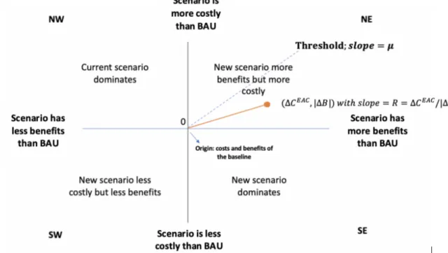
Benefits and costs are the two relevant decision parameters in our analysis. In principle, PET values as well as costs of new scenarios can be lower or higher than PET values and costs of the BAU scenario. This is shown in Figure 2 below.

Since we are interested in mitigating urban heat, no measure or scenario that results in a higher PET

value than the BAU will be considered as reasonable or eligible. Hence, the NW and SW sectors of the

plane in Figure 1 can be excluded. Among those scenarios, which yield a lower PET value than the

scenario “0” (sectors NE and SE), the ones with negative CER values (in the SE sector) would be most

preferable. They would represent a win-win situation in the sense that a lower PET value can be

achieved with lower costs than in the BAU scenario. The choice between different scenarios will have

to focus essentially on the SE and also the NE sectors in Figure 2.

Figure 2: Cost-Effectiveness plane diagram (Black, 1990)

Scenarios in the SE sector in Figure 2 are dominating the BAU scenario with respect to benefits and costs. They would hence be preferable for decision makers searching for urban heat mitigation measures.

Within the NE sector, those scenarios that lie on a rather low line (low gradient) are more preferable than others since they guarantee a given benefit at rather low additional costs. Hence, the gradient in the NE sector in Figure 2 would be a criterion for decision makers to look at. They should opt for scenarios that are on the lowest possible gradient line in the NE sector.

For the NE sector, there might be an additional requirement that the CER is below a threshold line (see

which would be an externally-set level of the maximum costs that are considered

acceptable for achieving a given reduction in PET. Such a threshold could, for instance, be derived

from the society's Willingness-To-Pay (WTP) for PET reductions. If such a threshold exists, decision

makers would have to make sure that chosen scenarios are below the respective line in the NE sector

of Figure 2.

Hence, the following decision rules for decision makers can be set up:

1) Choose dominating scenarios from the SE sector.

2) If there is no dominating scenario and there is a threshold for the CER, choose scenarios for which the respective CER is lower than the threshold 𝜇, i.e., those for which (2) holds:

𝐶𝐸𝑅

=

≤ 𝜇 (4)

3) If more than one scenario complies with rule (1) or rule (2), choose the scenario with the lowest CER, i.e., the one that is on the lowest gradient line. If two scenarios are on the same gradient, they are equally good from a CER perspective, although representing different levels of costs and benefits. Here it the depends on the question of how urgent PET value reductions are. The more urgent they seem to be, the more a scenario should be selected that is on the lowest gradient line and rather far to the right. Also benefit metrics 2 and 3 should be considered.

Apart from the decision rules just explained, we recommend that policy makers consider the secondary benefits of a scenario (i.e. energy consumption and greenhouse gas emissions).

As mentioned before, policy makers may consider the population’s WTP with respect to the implementation of urban heat mitigation measures (see Borzino et al, 2020 for details).

5 Results

In this sub-section, we present the results in costs, benefits and cost-effectiveness calculation for each the mitigation strategies under evaluation.

5.1 Electric Vehicles

5.1.1 Costs

Assumptions and simulation inputs

The timespan of electric vehicles is assumed to be 17 years because LTA vehicle registrations expire

after 17 years and buses cease operation after the registration expiry. As mentioned above, the discount

rate chosen in the assessment of costs is 3% (see Subsection 4.3 for details). In the estimation of costs,

we consider the costs faced by the government, the costs faced by the private sector and finally the

aggregated costs of both sides. We estimate the costs for the BAU and for each of the 5 scenarios

described in Section 3.2, Table 1.

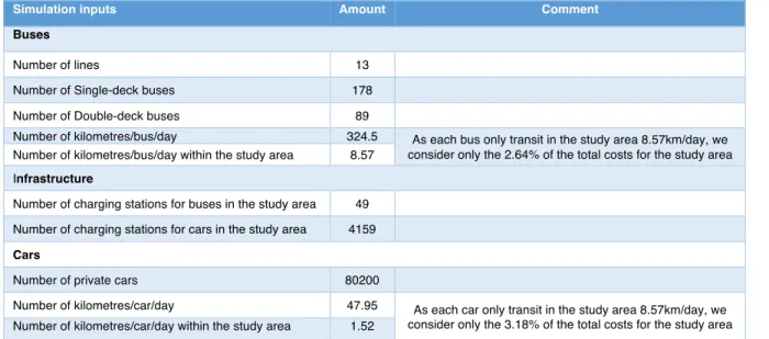
Only a small amount of the daily kms run by cars and buses refers to our study area. We only calculated the costs related to this study area. To do so, we first estimated CAPEX and OPEX costs for the buses and cars and for the total amount of kilometres per car and day. Then, we considered only 2.64% of the total costs for buses and 3.18% for cars, as these are the percentage of costs dedicated only to our study area (see Table 3).

Table 3: Simulation inputs for the calculation of costs.

Simulation inputs Amount Comment

Buses

Number of lines 13

Number of Single-deck buses 178

Number of Double-deck buses 89

Number of kilometres/bus/day 324.5 As each bus only transit in the study area 8.57km/day, we consider only the 2.64% of the total costs for the study area Number of kilometres/bus/day within the study area 8.57

Infrastructure

Number of charging stations for buses in the study area 49 Number of charging stations for cars in the study area 4159 Cars

Number of private cars 80200

Number of kilometres/car/day 47.95 As each car only transit in the study area 8.57km/day, we consider only the 3.18% of the total costs for the study area Number of kilometres/car/day within the study area 1.52

Following the simulation inputs from Table 3, we display the number of buses (both internal combustion engines (ICE) and electric vehicles (EV)) and cars (both ICE and EV) as well as the number of charging station for the BAU and each alternative scenario. Table 4 displays the number of cars, buses and charging station considered to estimate the costs and the benefits for each scenario. Once the total costs are estimated, we only count for 2.64% of the total costs for buses and for 3.18% of the total costs for cars given that only these percentages are costs relevant for the study site.

Table 4: Simulation inputs. Number of buses, cars and charging stations for the BAU and each scenario.

BAU S1 S2 S3 S4 S5

Number of:

No Electric Vehicles

33% of the fleet electrified 66% of the fleet non-electrified

66% of the fleet electrified 33% of the fleet non-electrified

100% of the fleet electrified

100% buses Electrified 100% of cars non-electrified

100% cars electrified 100% of buses

non-electrified

Double-deck bus ICE 89 60 29 - 29 89

Single-deck bus ICE 178 119 59 - 59 178

Double-deck bus EV - 29 60 89 - -

Single-deck bus EV - 59 119 178 - -

ICE cars 80200 52932 26466 - 80200 -

EV cars - 26466 52932 80200 - 80200

Charging stations EV buses - 16 32 49 49 -

Investment and Operational Costs

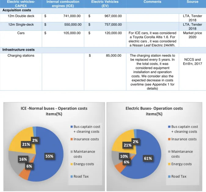
In the estimation of the costs, we considered CAPEX and OPEX of electric vehicles as described in Section 4.1. The description of each item, the assumptions as well as the sources are reported in Appendix 1. For the electric vehicles (EV), the CAPEX type of costs are the acquisition costs as well as the infrastructure costs. We report the CAPEX costs in Table 5.

We further report the OPEX costs for ICE and EV buses. EVs typically have low maintenance costs (see Appendix 1 for details). Hence, personnel costs (bus captain and cleaning staff) for EVs represent a higher percentage of the total operational costs compared with ICE vehicles. Figure 3 shows the respective shares for buses.

Table 5: Details of CAPEX (acquisition and infrastructure costs) for buses and cars.

Electric vehicles- CAPEX

Internal combustion engines (ICE)

Electric Vehicles (EV)

Comments Source

Acquisition costs

12m Double deck $ 741,000.00 $ 967,000.00 LTA, Tender 2018 12m Single-deck $ 550,000.00 $ 757,000.00 LTA, Tender

2018 Cars $ 105,000.00 $ 120,000.00 For ICE cars, it was considered

a Toyota Corolla Altis 1.6. For electric cars , it was considered

a Nissan Leaf Electric 24kWh.

Market price 2020

Infrastructure costs

Charging stations $ 85,000.00 The charging station needs to be replaced every 5 years. In

the total costs, it was considered equipment installation and operation costs. We consider also the expected decrease in costs overtime (see Appendix 1 for

details)

NCCS and Eri@n, 2017

Figure 3: Operational costs comparison between ICE and EV buses.

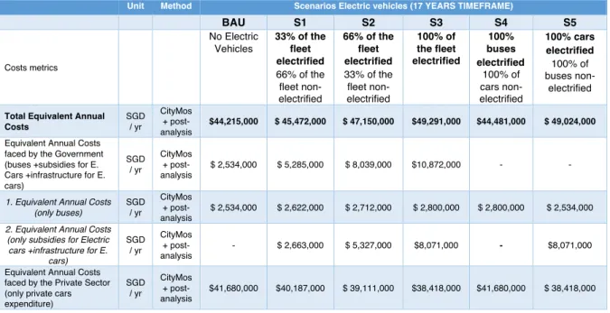
Equivalent Annual Costs

Table 6 presents the final EAC for the BAU scenario and each of the scenarios for the electric vehicles described in Table 1 and following Section 4.1. The costs presented in Table 6 are only the costs for the study site.

We calculated the aggregated EACs (for the government and for the private sector) as well as the EACs only faced by the government or the private sector. In the government costs, we considered the CAPEX and OPEX from the ICE and EV buses as well as the subsidies for the acquisition of electric cars and the tax rebates following Budget 2020 (Singapore Ministry of Finance, Singapore Budget, 2020).

Following the Singapore Budget 2020, we assumed that the subsidies for the acquisition of electric cars (i.e. SIN$20.000 per car) are given in time t=0, and that tax rebates for electric cars (i.e. SGD$ 100 in the first year; SGD$200 in the second year and SGD$350 from the third year on) are given for the 17 years’ timeframe.

The EACs faced by the private sector are assumed to be composed of the non-subsidized acquisition costs for the ICE cars and EV cars and of the operational costs (maintenance, road tax, insurance and petrol/electricity).

Table 6: Equivalent Annual Costs for electric vehicles in the study site. Private sector costs, public sector costs and aggregated costs for BAU and each scenario.

Unit Method Scenarios Electric vehicles (17 YEARS TIMEFRAME)

BAU S1 S2 S3 S4 S5

Costs metrics

No Electric Vehicles

33% of the fleet electrified 66% of the fleet non- electrified

66% of the fleet electrified 33% of the fleet non- electrified

100% of the fleet electrified

100%

buses electrified

100% of cars non- electrified

100% cars electrified 100% of buses non-

electrified Total Equivalent Annual

Costs

SGD / yr

CityMos + post- analysis

$44,215,000 $ 45,472,000 $ 47,150,000 $49,291,000 $44,481,000 $ 49,024,000

Equivalent Annual Costs faced by the Government (buses +subsidies for E.

Cars +infrastructure for E.

cars)

SGD / yr

CityMos + post- analysis

$ 2,534,000 $ 5,285,000 $ 8,039,000 $10,872,000 - -

1. Equivalent Annual Costs (only buses)

SGD / yr

CityMos + post- analysis

$ 2,534,000 $ 2,622,000 $ 2,712,000 $ 2,800,000 $ 2,800,000 $ 2,534,000 2. Equivalent Annual Costs

(only subsidies for Electric cars +infrastructure for E.

cars)

SGD / yr

CityMos + post- analysis

- $ 2,663,000 $ 5,327,000 $8,071,000 - $8,071,000

Equivalent Annual Costs faced by the Private Sector (only private cars expenditure)

SGD / yr

CityMos + post- analysis

$41,680,000 $40,187,000 $ 39,111,000 $38,418,000 $41,680,000 $ 38,418,000

Table 6 shows the total EAC for each of the scenarios evaluated for the study site (first line in Table 6).

The EAC values increase progressively as the percentage of electrification of the fleet increases. The values increase by 2.84%, 6.64% and 11.48% in S1, S2 and S3 compared with the BAU scenario. The EAC increase sonly by 0.60% in the scenario S4 and by 10.88% in the scenario S5, both compared with the BAU scenario. Comparing the S3 and S5 scenarios (i.e., all vehicles electrified or only the cars electrified, respectively), we see that the difference between those two is only 0.6%.

Table 6 also displays the EAC values faced only by the government (line 2 in Table 6) and also those faced only by the private sector (line 5 in Table 6), both for each scenario.

However, for the analysis done in this study, we only discuss the total EAC, i.e. the total equivalent annualised costs faced by government and private households in the BAU and each urban heat reducing scenario.

5.1.2 Cost-effectiveness calculation

In this subsection, we apply the Cost-effectiveness calculation described in Section 4.1. By implementing this framework, we evaluate the cost-effectiveness of each scenario (i.e., S1 to S5) compared with the BAU scenario for the electrification of the vehicle fleet.

In the upper part of Table 7, we display the results from the costs metrics (i.e., total EAC) for the BAU scenario and for the alternative scenarios considered S1 to S5. We discussed the EAC estimations for BAU and each of the implementation scenarios in Section 5.1.1.

In the middle part of Table 7, we display the results from the benefit calculations, i.e., the PET values (as indicator for outdoor thermal comfort), the energy consumption and the greenhouse gas emissions.

We display the results of each of these metrics for the BAU and per each implementation scenario (S1 to S5) (for more details see Adelia et al., 2020).

We observe that the lowest PET value is obtained by the implementation of a 100% electrification of

the vehicle fleet. We observe a 0.91 C° decrease in PET in the respective scenario (i.e., S3), compared

with the BAU scenario. We also see a 0.71 C° PET decrease in the scenario with only electrified buses

(100%) (S4) and a 0.81 C° PET decrease in the scenario with only electrified cars (100%) (S5), both

compared with the BAU scenario.

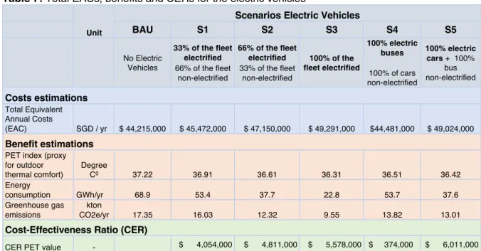
Table 7: Total EACs, benefits and CERs for the electric vehicles

Unit

Scenarios Electric Vehicles

BAU S1 S2 S3 S4 S5

No Electric Vehicles

33% of the fleet electrified 66% of the fleet

non-electrified

66% of the fleet electrified 33% of the fleet

non-electrified

100% of the fleet electrified

100% electric buses 100% of cars non-electrified

100% electric cars + 100%

bus non-electrified Costs estimations

Total Equivalent Annual Costs

(EAC) SGD / yr $ 44,215,000 $ 45,472,000 $ 47,150,000 $ 49,291,000

$44,481,000 $ 49,024,000 Benefit estimations

PET index (proxy for outdoor thermal comfort)

Degree

C⁰ 37.22 36.91 36.61 36.31 36.51 36.42

Energy

consumption GWh/yr 68.9 53.4 37.7 22.8 53.7 37.6

Greenhouse gas emissions

kton

CO2e/yr 17.35 16.03 12.32 9.55 13.82 13.01

Cost-Effectiveness Ratio (CER)

CER PET value - $ 4,054,000 $ 4,811,000 $ 5,578,000 $ 374,000 $ 6,011,000

We also display the additional benefits that come along with the implementation of electric vehicles in the study site. In Table 7, we see that energy consumption and greenhouse gas emissions decrease significantly with the implementation of the different new technology scenarios. The more the fleet is electrified, the lower are the energy consumption and the greenhouse gas emissions. The reduction in energy consumption amounts to 66.91%, 22.01% and 45.43% for the scenarios S3, S4 and S5 respectively, compared with the BAU scenario.

The greenhouse gas emissions decrease with an increasing degree of fleet electrification. The 100%

electrification scenario (S3) presents a 44.96% reduction in GHG emissions compared with the BAU scenario. If only 100% of the buses are electrified (S4) or only 100% of the private cars are electrified (S5), we obtain an emission reduction of 20.35% or 25.02% compared with the BAU scenario.

The bottom part of Table 7 reports the cost-effectiveness ratio (CER) calculated following Equation (3) in Section 4.2. The CER shows the costs, which have to be paid for a 1-degree C° reduction of the PET indicator compared with the BAU scenario. As the scenarios S1 – S5 present an improvement of the PET value at higher costs, those scenarios lie in the NE sector of Figure 2. This means that we should select scenarios that lie on the lowest gradient line.

In the last row of Table 7, we see that the CER increases as the percentage of the fleet electrification

increases (from S1 to S3). The CER in the 100% fleet electrification scenario (S3) is 37.59% higher

Scenario S1 seems preferable as it presents a lower cost per 1-degree PET improvement. However, the picture changes if we consider the additional benefits that come with a higher degree of fleet electrification (for instance S3). As described above, scenario S3 brings a significant decrease in energy consumption and in greenhouse gas emissions compared with the BAU and S1 scenarios.

In the last row of Table 7, we also report the CER results for the electrification of buses only (S4) and the electrification of cars only (S5). We observe that the additional costs per degree of PET improvement are only SGD 374.000 in S4 compared with the BAU scenario. The total electrification of buses also brings a significant reduction in both energy conservation and greenhouse gas emissions.

In the case in which only cars are electrified (S5), we observe a CER of around SGD 6m. The respective CER is higher than the CER resulting from the 100% fleet electrification (S3). This result suggests that it might be more preferable to electrify the entire fleet instead of electrifying cars only. This holds even more if the additional benefits are taken into account.

Overall, our results suggest that the electrification of buses only (S4) might be the most preferable scenario: it presents the lowest CER across all scenarios along with significant additional benefits for the environment, like a decrease in energy consumption and a decrease in greenhouse gas emissions compared with the BAU scenario.

The scenario that presents the highest improvement in OTC is the 100% electrification of the fleet (S3), but it comes with higher costs and a higher CER value. For S3, the reductions in energy consumption as well as in GHG emissions are the highest among S1 to S5. It seems recommendable to consider these benefits in addition to the CER value. Policy makers would need a weighting scheme for the three benefit metrics in order to make a rational choice of an urban heat mitigation measure.

5.2 District Cooling Systems

In this Subsection, we show the costs, benefits and cost-effectiveness calculations for District Cooling Systems. We display the results for different scenarios. More details about the District Cooling Systems, along with their Capex and Opex costs, can be found in the “Potential of District Cooling in Singapore:

From Micro to Mesoscale” Technical Report from the Cooling Singapore project produced by

5.2.1 Costs

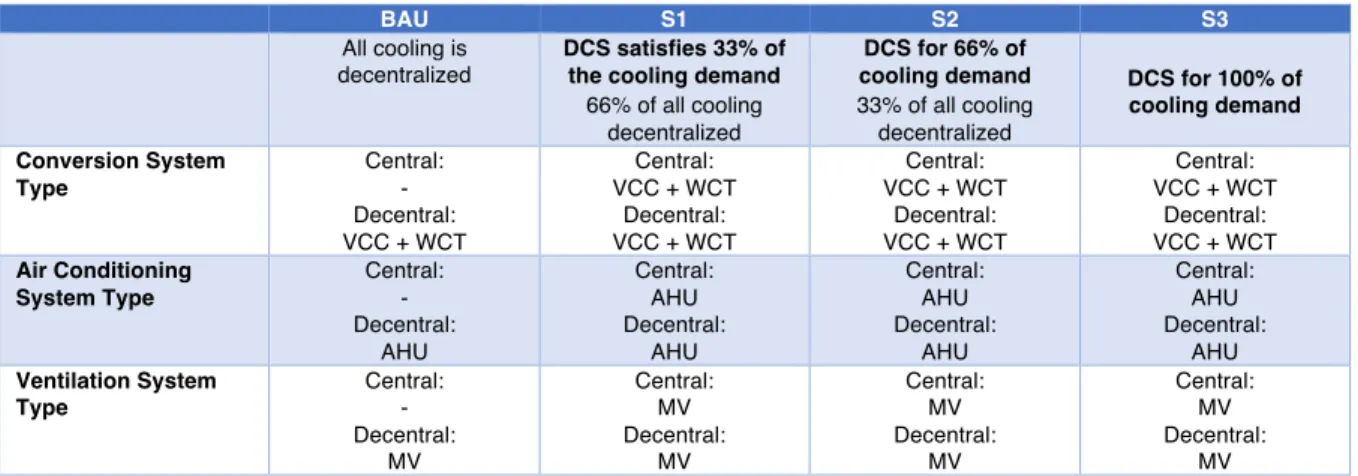
Assumptions about technologies

Following Riegelbauer et al . , 2020, the cooling system of an area is a combination of three main sub- systems. These are the Conversion System, the Air-Conditioning System, and the Ventilation System.

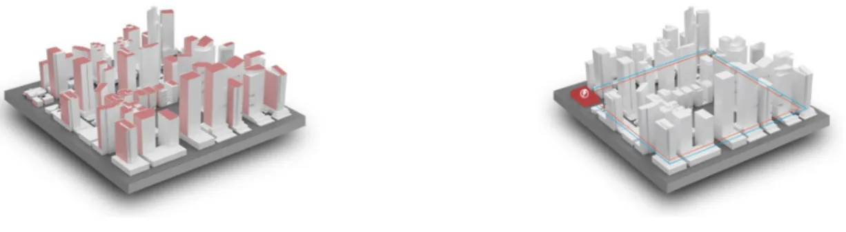
Table 8 and Table 9 indicate the type of technologies used per sub-system, scenario, and land-use in the study area. We also describe the type of technology used for centralized buildings (i.e., buildings that are connected to a central District Cooling System) and for decentralized buildings (i.e., buildings that are not connected to a central District Cooling System) (see Figure 4).

Figure 4: Schematic presentation of cooling systems’ location (in red) in decentralized (left) and centralized (right) buildings in the study area.

The BAU scenario with respect to district cooling represents the most commonly used cooling systems of Singapore's building stock today. These cooling systems are decentralized per building and, as such, no district cooling schemes. For residential buildings, the BAU scenario's conversion system uses Direct Expansion Units (DEX) to reject heat into the outdoor environment. The air conditioning system uses a Fan coil or mini-split unit (FC), which is typical for residential units. The ventilation system consists of natural ventilation (NV).

On the other hand, for commercial buildings, the BAU scenario's conversion system consists of a combination of vapour compression chillers (VCC) and Wet cooling towers (WCT) to reject heat into the outdoor environment. The air conditioning system uses an air handling unit (AHU), typical for medium-size and large commercial units, including retail, hotels, and offices. The ventilation system consists of traditional mechanical ventilation with metallic ducting and electrical fans (MV).

At the side of the BAU scenario, we also consider 33%, 66% and 100% scenarios for district cooling.

As before, we name them S1, S2 and S3. The 33% district cooling scenario portrays an integration of

The scenario includes a remaining 66% of the buildings using typical cooling systems as they are used in Singapore today. For both commercial and residential buildings connected to the centralized District Cooling System, the scenario's conversion system uses VCC and WCT, the air conditioning system uses AHU, and the ventilation system is MV. For commercial and residential buildings not connected to the District Cooling System (DCS) (decentralized), the cooling system is the same as described for the BAU scenario.

The 66% and 100% district cooling scenarios follow the same rationality of the 33% scenario regarding the cooling system technology and configurations.

Table 8: Technologies used in each scenario at the decentralized and centralized scales for Residential buildings.

DEX: Direct expansion unit. VCC: Vapour compression chiller. WCT: Wet cooling tower. FC: Fan coil mini-split unit. NV: Natural ventilation. MV: mechanical ventilation. AHU: air conditioning system uses an air handling unit.

Table 9: Technologies used in each scenario at the decentralized and centralized scales for Commercial buildings.

DEX: Direct expansion unit. VCC: Vapour compression chiller. WCT: Wet cooling tower. FC: Fan coil mini-split unit. NV: Natural ventilation. MV: mechanical ventilation. AHU: air conditioning system uses an air handling unit.

BAU S1 S2 S3

All cooling is decentralized

DCS satisfies 33% of the cooling demand

66% of all cooling decentralized

DCS for 66% of cooling demand 33% of all cooling decentralized

DCS for 100% of cooling demand Conversion System

Type

Central:

- Decentral:

DEX

Central:

VCC + WCT Decentral:

DEX

Central:

VCC + WCT Decentral:

DEX

Central:

VCC + WCT Decentral:

- Air Conditioning

System Type

Central:

- Decentral:

FC

Central:

AHU Decentral:

FC

Central:

AHU Decentral:

FC

Central:

AHU Decentral:

- Ventilation System

Type

Central:

- Decentral:

NV

Central:

MV Decentral:

NV

Central:

MV Decentral:

NV

Central:

MV Decentral:

-

BAU S1 S2 S3

All cooling is decentralized

DCS satisfies 33% of the cooling demand 66% of all cooling

decentralized

DCS for 66% of cooling demand 33% of all cooling decentralized

DCS for 100% of cooling demand Conversion System

Type

Central:

- Decentral:

VCC + WCT

Central:

VCC + WCT Decentral:

VCC + WCT

Central:

VCC + WCT Decentral:

VCC + WCT

Central:

VCC + WCT Decentral:

VCC + WCT Air Conditioning

System Type

Central:

- Decentral:

AHU

Central:

AHU Decentral:

AHU

Central:

AHU Decentral:

AHU

Central:

AHU Decentral:

AHU Ventilation System

Type

Central:

- Decentral:

MV

Central:

MV Decentral:

MV

Central:

MV Decentral:

MV

Central:

MV Decentral:

MV

Assumptions about specific technology costs

Table 10 presents the specific costs and cost calculation parameters of the cooling systems analysed in this study. We follow a simplified approach, where the investment costs are defined per unit of thermal capacity installed. The costs include design fees, contingencies, and taxes (Riegelbauer et al, 2020 for more details of these cost items).

We are confronted with two types of investment costs for a decentralized cooling of buildings. The investment costs of the system ‘VCC + WCT + AHU + MV for buildings that are cooled in a decentralized way comprise costs for vapour compression chillers, cooling towers, chilled water pumps, chilled water pipework, condenser water pumps, and condenser water pipework for the conversion component of the cooling system (see

conditioning system costs, namely the air handling unit, air conditioning ductwork, and automatic control works (see Riegelbauer et al, 2020 for more details).

The investment costs of the system ‘DEX + FC + NV for buildings that are cooled in a decentralized way comprise costs for condenser units, indoor units, and piping. They do not include the costs of concealing piping, which is allocated to the inherent construction costs of building developers (see

Table 10: Specific costs per technology and cooling system.

DEX: Direct expansion unit. VCC: Vapour compression chiller. WCT: Wet cooling tower. FC: Fan coil mini-split unit. NV: Natural ventilation.

MV: mechanical ventilation. NETWORK: District Cooling network. ELECTRICITY: electricity.

* Cooling operators with a monthly electricity consumption above 2000 kWh/month are assumed to purchase electricity from the open electricity market, benefitting of reduced rates

2 https://www.openelectricitymarket.sg/business/list-of-retailers#business-consumers-min-2000

Item Specific

Cost [SGD/kW]

Lifetime [LT]

O&M [%]

Discount Rate [%]

Source

VCC + WCT + AHU + MV

for decentralized buildings 1170 20 4% 3% (Arcadis 2016)

DEX + FC + NV

For decentralized buildings 380 15 12% 3% Retailer

VCC + WCT + NETWORK + MV For centralized buildings

2080 50 2% 3% (ASHRAE, 2009,

Arcadis 2016⁾ ELECTRICITY

For centralized and decentralized buildings

0.25/0.188* - - - EMA², OEM³

The investment cost of the system ‘VCC + WCT + NETWORK + MV for buildings that are cooled in a centralized way, i.e. the district cooling system investment costs comprise costs for the District Cooling System, the district cooling network, energy transfer stations, and a share of the central air conditioning system of buildings. The lifetime of the entire system is estimated to be 50 years, even though single components might deviate (see Fonseca et al., 2020; Riegelbauer et al, 2020). This estimation is mainly due to the long-term duration of fixed investment components of the District Cooling Systems’

infrastructure (i.e. district cooling network, energy transfer stations, and the central air conditioning systems of buildings) as declared by district cooling providers (Tabreed, 2018). The operational and maintenance percentage of the total costs amounts to 2% (Ashrae, 2009). It is low compared to decentralized cooling systems, which show a share of 22.8% for operational and maintenance costs compared to the total costs (see Riegelbauer et al, 2020).

Since all systems are electrically powered, the electricity price is pivotal in analysing the costs. In Singapore, large consumers with a monthly electricity consumption above 2000 kWh/month are allowed to purchase electricity from the open electricity market, benefitting from reduced rate

. We assume that all cooling operators, who meet this criterion, benefit of a 25% price reduction compared to the standard electricity tariff

(see Riegelbauer et al, 2020).

Investment costs

Regarding investment costs, we assume all cooling systems for our study area to be installed in period

0. A trend of increasing investment costs with an increasing share of buildings belonging to the district

cooling system can be observed in Figure 5. Scenario S3, the scenario in which 100% of the cooling

demand is satisfied by a centralized system, is the most capital intensive scenario (see Riegelbauer et

al, 2020). The total capital expenditure amounts to approximately 1.48 billion SGD for the entire district

cooling system, while cooling systems in the BAU scenario account for investment costs of 790 million

SGD. Decisive for this gap is the investment for the district cooling network and the energy transfer

stations (see Riegelbauer et al, 2020).

Figure 5: Investment costs for all scenarios (source: Riegelbauer et al., 2020).

BAU: Business as usual scenario; S1: 33% district cooling scenario; S2: 66% district cooling scenario; S3: 100% district cooling scenario. CapEx [Decentral]: Investment or capital costs for locally cooled buildings. CapEx [Central]:

Investment or capital costs for centrally cooled buildings.

Operational costs

For cooling systems, the operational or running costs per year decrease with an increase in the district cooling share (see Figure 6). This cost decrease can be attributed to the efficiency improvements of district cooling systems, which result in a lower electricity consumption of the cooling system (see

costs are low, compared to buildings that are cooled in a decentralized way (see Riegelbauer et al, 2020).

Figure 6: Operational costs for all scenarios (source: Riegelbauer et al., 2020).

BAU: Business as usual scenario. S1: 33% district cooling scenario. S2: 33% district cooling scenario. S3: 100% district cooling scenario. OPEX Fix [Decentral]: Fixed operational costs for locally cooled buildings. OPEX Fix [Central]: Fix